Progress on a Conjecture Regarding the Triangular Distribution

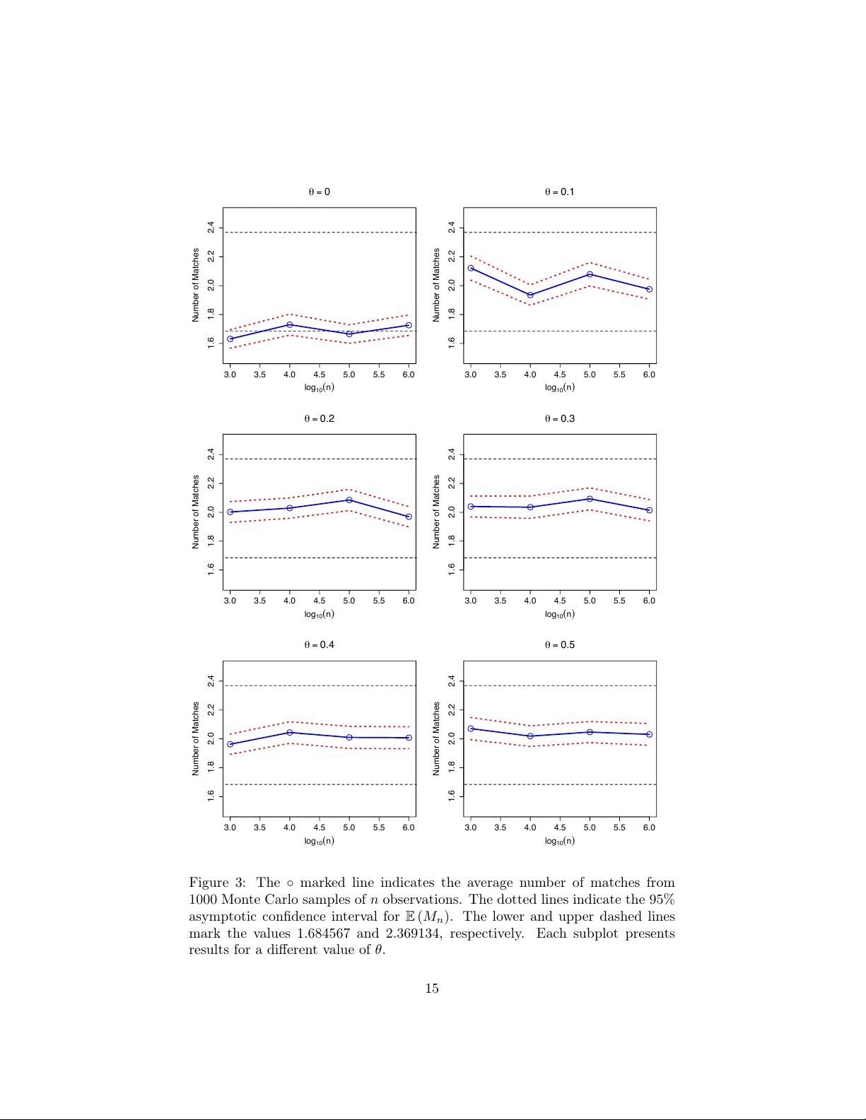
Progress on a Conjecture Regarding the T riangular Distribution Hien D. Nguy en 1 , 2 and Geoffrey J. McLac hlan 1 No v em b er 5, 2016 1 Sc ho ol of Mathematics and Ph ysics, Univ ersit y of Queensland. 2 Cen tre for A dv anced Imaging, Univ ersity of Queensland. Abstract T riangular distributions are a w ell-known class of distributions that are often used as an elemen tary example of a probability mo del. Maximum lik eliho o d estimation of the mo de parameter of the triangular distribu- tion ov er the unit in terv al can b e performed via an order statistic-based metho d . It had b een conjectured that suc h a metho d can b e conducted using only a constant n umber of likelihoo d function ev aluations, on a v- erage, as the sample size b ecomes large. W e pro ve tw o theorems that v alidate this conjecture. Graphical and n umerical results are presen ted to supplemen t our pro ofs. 1 In tro duction Let X ∈ [0 , 1] b e a random v ariable with cumulativ e distribution function (CDF) 1 F θ ( x ) =        x 2 /θ , if x < θ , 1 − (1 − x ) 2 / (1 − θ ) , if x ≥ θ , (1) when θ ∈ (0 , 1) , F 0 ( x ) = 1 − (1 − x ) 2 when θ = 0 , and F 1 ( x ) = x 2 when θ = 1 . W e sa y that X arises from a triangular distribution with mo de parameter θ ∈ [0 , 1] . The probability density function of X can b e written as f θ ( x ) =        2 x/θ , if x < θ , 2 (1 − x ) / (1 − θ ) , if x ≥ θ , when θ ∈ (0 , 1) , f 0 ( x ) = 2 (1 − x ) when θ = 0 , and f 1 ( x ) = 2 x when θ = 1 . The triangular distribution is a p opular probability model for teaching, due to its simple geometric form; see Doane (2004) and Price and Zhang (2007) for examples where the triangular distribution is used in the teaching of v arious asp ects of distribution theory . Outside of the classro om, the triangular distribu- tion has also been used to mo del task completion times for Program Ev aluation and Review T ec hniques (PER T) mo dels, prices of securities that are traded on the New Y ork Sto ck Exchange, and haul times in civil engineering data. Elab- orations on these applications can b e found in Kotz and V an Dorp (2004, Ch. 1) and the references therein. Recen tly , there has b een a renew ed interest in the triangular distribution. F or example, Glic kman and Xu (2008) inv estigated the distribution of the prod- uct of triangular distributions for applications in traffic-related risk assessment, Karlis and Xek alaki (2008) considered the use of mixtures of triangular distri- butions for estimation of b ounded and concav e densities, and Nagara ja (2013) deriv ed expressions for the momen ts of order statistics and L-moments, for appli- cation smart communication net w orks. F urthermore, Gunduz and Genc (2015) follo wed the work of Glickman and Xu (2008) and derived expressions for the 2 distribution of quotients of triangular distributions, and Nguy en and McLachlan (2016) utilized a nov el c haracterization of the triangular distribution to derive minorization–maximization algorithms (Hunter and Lange, 2004) for the maxi- m um likelihoo d (ML) estimation of the triangular distribution and the mixture of triangular distributions of Karlis and Xek alaki (2008). Let X 1 , ..., X n b e a random I ID (indep endent and identically distributed) sample of size n ∈ N from a triangular distribution with unknown mo de param- eter and let x 1 , ..., x n b e its realization. The likelihoo d function and the ML estimator can b e expressed as L n ( θ ) = Q n i =1 f θ ( x i ) and ˆ θ n = arg max θ ∈ [0 , 1] L n ( θ ) , resp ectiv ely . Let x (1) ≤ x (2) ≤ ... ≤ x ( n ) b e the order statistics of the sample realization. It is sho wn in Oliver (1972) that ˆ θ n = x ( i ) for some i = 1 , ..., n . That is, the ML estimate is alwa ys one of the observ ations from sample; the same result was pro ved in Kotz and V an Dorp (2004, Ch. 1). Remark ably , Oliv er (1972) also sho wed that if ˆ θ n = x ( j ) , then x ( j ) m ust fulfill the condition ( j − 1) /n < x ( j ) < j /n . Thus, the ML estimator can b e rewritten as ˆ θ n = arg max θ ∈ Θ n L n ( θ ) (2) where Θ n =  x ( j ) : ( j − 1) /n < x ( j ) < j /n, j = 1 , ..., n  . An in v estigation into the exp ected n umber of elemen ts in the set Θ n w as con- ducted by Huang and Shen (2007). Let m n = P n j =1 I  ( j − 1) /n < x ( j ) < j /n  b e the observed num ber of elemen ts in Θ n , where I { A } equals 1 if prop osition A is true and 0 otherwise. As with Huang and Shen (2007), we wi ll sub sequen tly 3 call m n the observed num ber of ’matches’. It was observ ed and conjectured that E ( M n ) = n X j =1 P  j − 1 n < X ( j ) < j n  ≈ 2 (3) as n grows large, for v arious v alues of θ . Here X (1) ≤ X (2) ≤ ... ≤ X ( n ) is the or- der statistics of a random sample, and M n = P n j =1 I  ( j − 1) /n < X ( j ) < j /n  . In contrast to this observ ation regarding the triangular distribution, Huang and Shen (2007) pro v ed that if one assumes that X 1 , ..., X n is an I ID sample from a uniform distribution ov er the unit interv al (i.e. X ∈ [0 , 1] ), then the exp ected num b er of elements in Θ n is E ( M n ) = 1 + n − 1 X j =1  n j   j n  j  1 − j n  n − j . (4) Up on application of Stirling’s form ula [cf. Charalam bides (2002, Thm. 3.2)] and lim n →∞ P n − 1 j =1 1 / p j ( n − j ) = π , Huang and Shen (2007) obtained the appro ximation form ula E ( M n ) ≈ 1 + r n 2 π n − 1 X j =1 1 p j ( n − j ) ≈ 1 + r π n 2 (5) for large n . Thus, whereas the exp ected n um b er of matches for a triangular distribution remains constant as n grows, the expected num ber of matches grows at a rate of O ( √ n ) [using Landau’s O-notation; see Cormen et al. (2002, Ch. 3)] asymptotically , when the sample arises from a uniform distribution. In Nguyen and McLachlan (2016), it was established that the av erage or- der of complexity for computing the ML estimate using the estimator (2) is O ( n [log n + E ( M n )]) . This is due to the requiremen t of a sorting algorithm to obtain the order statistics, which requires O ( n log n ) op erations [e.g. Heapsort (Cormen et al., 2002, Ch. 6, p. 146)], and the computation of the lik eliho o d 4 function for comparison, whic h requires O ( n ) op erations. Thus, if the conjec- ture of Huang and Shen (2007) is true (i.e. (3) is true), then the ML estimate has av erage order of complexity O ( n log n ) , which makes it no more complex than the computation of order statistics. In this article, we extend the w ork of Huang and Shen (2007) to obtain an expression for the exp ected n umber of matches E ( M n ) of samples arising from an y distribution o v er the unit in terv al. F urthermore, w e prov e that for any con tinuous distribution, the maximum rate of growth of E ( M n ) is O ( √ n ) . Using the deriv ed general expression for E ( M n ) , we provide a formula for the exp ected num ber of matches of an y sample arising from a triangular distribution. Using the formula, w e then pro v e that E ( M n ) → 1 . 684567 , as n → ∞ , for θ ∈ { 0 , 1 } . Similarly , for θ ∈ (0 , 1) , we obtain the approximation E ( M n ) ≈ N n for large n , where N n → 2 . 369134 , as n → ∞ . Thus, w e obtain p ositive progress to wards the conjecture of Huang and Shen (2007). W e supplement the main result with graphical and numerical results regarding the expected n um b er of matc hes from a triangular distributed sample. Although the conten t of the article is aimed at resolving the discussed con- jecture of Huang and Shen (2007), it is anticipated that the techniques from this article can also b e applied in other settings. The standard tw o-sided p ow er distribution (STPD) of Kotz and V an Dorp (2004, C h. 3) is a generalization of the triangular distribution for which the ML estimator is an order statistic that satisfies a criterion [cf. K otz and V an Dorp (2004, Ch. 3, p. 80)]. It ma y b e p ossible to apply the metho dology from this article to obtain an analo- gous result in the S TPD setting. The b eta distribution is also interesting as it includes b oth the θ ∈ { 0 , 1 } cases of the triangle as well as the uniform distri- bution as sp ecial cases. An interesting problem that arises is to determine the parameter settings for which the num ber of matches E ( M n ) conv erges in the 5 b eta distribution setting. The rest of the article pro ceeds as follows. General results regarding the exp ected num ber of matches that are obtained from arbitrary distributions o ver the unit interv al are presented in Section 2. Sp ecific results regarding the trian- gular distribution are presented in Section 3. Numerical and graphical results are presen ted in Section 4. Pro ofs for the main results are relegated to Section 5. 2 General Results Let X 1 , ..., X n b e an I ID random sample, where X 1 ∈ [0 , 1] has distribution function F ( x ) , which is well-defined for x ∈ [0 , 1] . Let, X (1) ≤ X (2) ≤ ... ≤ X ( n ) b e the order statistics of the random sample. F or j = 1 , ..., n , let F j : n ( x ) b e the distribution function of X ( j ) . David and Nagara ja (2003, Eq. 2.1.3) states F j : n ( x ) = n X i = j  n i  F i ( x ) [1 − F ( x )] n − i , (6) whic h pro vides the link b et w een F ( x ) and the order statistic distributions. Using (6), we get the general formula for the exp ected num ber of matc hes of an y sample arising from distribution F ( x ) . Theorem 1. L et X 1 , ..., X n b e an IID r andom sample, wher e X 1 ∈ [0 , 1] has distribution F ( x ) .The exp e cte d numb er of matches fr om the sample is E ( M n ) = 1 + n − 1 X j =1  n j  F j  j n   1 − F  j n  n − j . (7) R emark 1 . If X 1 has distribution F ( x ) = x (i.e. X 1 is uniformly distributed), then (7) b ecomes (4), as exp ected. Via an elementary calculus argument and up on application of Stirling’s for- 6 m ula, we obtain the follo wing upp er b ound for the asymptotic gro wth rate of the exp ected num ber of matches. Corollary 1. L et X 1 , ..., X n b e an IID r andom sample, wher e X 1 ∈ [0 , 1] has distribution F ( x ) . F or any F ( x ) , the asymptotic gr owth r ate of E ( M n ) has up- p er b ound O ( √ n ) . F or lar ge n , the u pp er b ound of E ( M n ) c an b e asymptotic al ly appr oximate d by Equation (5). R emark 2 . Corollary 1 implies that the uniform distribution maximizes the gro wth rate of the exp ected n umber of matches. Interestingly , the right-hand side of (5) is related to the enumeration of ro oted trees by total height. That is, n p π n/ 2 is the asymptotic gro wth rate of the mean total heigh t of all ro oted trees with n lab eled p oints, and also the mean height; see Riordan and Sloane (1969). F urthermore, up on rearrangemen t of Equation (4), we obtain the OEIS (On-line Encyclop edia of Integer Sequences; https://oeis.org) sequence A001864 from the expression n n ( E ( M n ) − 1) ; see also M2138 from Sloane and Plouffe (1995). 3 T riangular Distribution Let X 1 , ..., X n b e an I ID random sample, where X 1 has triangular distribution function F θ ( x ) . F rom Theorem 1, we hav e E ( M n ) = 1 + n − 1 X j =1  n j  F j θ  j n   1 − F θ  j n  n − j . (8) In the case where θ = 0 or θ = 1 , (8) b ecomes E ( M n ) = 1 + n − 1 X j =1  n j  " 1 −  1 − j n  2 # j  1 − j n  2( n − j ) 7 and E ( M n ) = 1 + n − 1 X j =1  n j   j n  2 j " 1 −  j n  2 # n − j = 1 + n − 1 X j =1  n n − j   n − j n  2( n − j ) " 1 −  n − j n  2 # j = 1 + n − 1 X j =1  n j  " 1 −  1 − j n  2 # j  1 − j n  2( n − j ) , (9) resp ectiv ely . It is not difficult to obtain the limit lim n →∞  n j  " 1 −  1 − j n  2 # j  1 − j n  2( n − j ) = 2 j e − 2 j j j j ! = s j . Th us, w e ha ve E ( M n ) ≈ 1 + S n − 1 (10) for large n in the cases where θ ∈ { 0 , 1 } , and S n = P n j =1 s j . Lemma 1. The series S n c onver ges to S ∞ ≈ 0 . 684567 . Applying Lemma 1 to (10) yields the first main result of the article. Theorem 2. F or triangular distributions with θ ∈ { 0 , 1 } , E ( M n ) → 1 . 684567 , as n → ∞ . Supp ose now that n = p + q and let θ = p/ ( p + q ) , where p, q ∈ N . F rom (1), we note that F θ ( θ ) = θ ; thus θ is the θ th quantile of the distribution. Using 8 this fact, we hav e the following expression of (8): E ( M p + q ) = 1 + p X j =1  p + q j  F j θ  j p + q   1 − F θ  j p + q  p + q − j + p + q − 1 X j = p +1  p + q j  F j θ  j p + q   1 − F θ  j p + q  p + q − j = 1 + p X j =1  p + q j  F j 1  j p   1 − F 1  j p  p + q − j + p + q − 1 X j = p +1  p + q j  F j 0  j q   1 − F 0  j q  p + q − j = 1 + p X j =0  p + q p − j   p − j p  2( p − j ) " 1 −  p − j p  2 # q + j + q − 1 X j =1  p + q p + j  " 1 −  1 − p + j q  2 # p + j  1 − p + j q  2( q − j ) . The second equality is due to the fact that the first θ = p/ ( p + q ) is the [ p/ ( p + q )] th quantile. W e apply this fact by noting that f θ ( x ) , to the left of θ , has up w ards-sloping densit y and vice v ersa, has do wn w ard-sloping densit y to the right. Since all triangular distributions must hav e heigh t f θ ( θ ) = 2 , the region to the left of θ is prop ortional f 1 ( x ) in the sense that f θ ( x ) = f 1 ( y ) , for x = θ y , and similarly the region to the right is prop ortion to f 0 ( x ) in the sense that f θ ( x ) = f 0 ( y ) , for x = (1 − θ ) y . Via the prop ortionality argument, w e can compute F θ  j n  = F 1  j n × n p  = F 1  j p  , for j /n ≤ θ , and F θ  j n  = F 0  j n × n q  = F 0  j q  , for j /n > θ . 9 Again, it is not difficult to obtain the limits lim p →∞  p + q p − j   p − j p  2( p − j ) " 1 −  p − j p  2 # q + j = 2 j + q e − 2 j j j + q ( j + q )! = u q j and lim q →∞  p + q p + j  " 1 −  1 − p + j q  2 # p + j  1 − p + j q  2( q − j ) = 2 j + p e − 2( j + p ) ( j + p ) j + p ( j + p )! = v p j . Th us, w e ha ve E ( M p + q ) ≈ 1 + U q p + V p q , (11) where U q p = P p j =1 u q j and V p q = P q j =1 v p j , for large p and q . Note that U q p is indexed from j = 1 , since 0 0+ q = 0 for any q ∈ N . Lemma 2. The series U q p c onver ges as p → ∞ , for any finite q ∈ N , and the series V p q c onver ges as q → ∞ , for any finite p ∈ N . F or fixed j , w e note that u q j /s j = 2 q j q j ! / ( j + q )! → 0 , as q → ∞ since factorials gro w faster than exp onentials. Similarly v p j /s j → 0 , as p → ∞ . Thus, w e obtain the following result. Lemma 3. The r atios u q j /s j → 0 and v p j /s j → 0 , as q → ∞ and p → ∞ , r esp e ctively, for any finite j ∈ N . Lemmas 2 and 3 suggest that for large p and q , E ( M p + q ) conv erges to a finite constan t. F urther, it is suggested that we can conserv ativ ely appro ximate E ( M p + q ) by N p,q = 1 + S p + S q , in the sense that 1 + U q p + V p q ≤ N p,q for large p and q . An application of Lemma 1 yields the second main result of the article. Theorem 3. F or triangular distributions with θ = p/ ( p + q ) for p, q ∈ N , E ( M p + q ) ≈ N p,q , wher e N p,q → 2 . 369134 , as p → ∞ and q → ∞ . 10 T able 1: Exact v alues of exp ected matches E ( M n ) for v arious sample sizes n and mo de parameters θ . n \ θ 0 0.1 0.2 0.3 0.4 0.5 5 1.814694 1.960713 2.093680 2.162657 2.207036 2.217071 10 1.929234 2.271707 2.466275 2.579562 2.640312 2.659541 20 1.842068 2.394180 2.608803 2.707651 2.751632 2.764140 50 1.731881 2.490839 2.531784 2.487879 2.450077 2.436588 100 1.705885 2.477835 2.358059 2.282239 2.249001 2.239780 200 1.694797 2.332438 2.205683 2.166804 2.151832 2.147659 500 1.688567 2.162322 2.110494 2.093518 2.086342 2.084280 1000 1.686553 2.103114 2.073165 2.062607 2.058058 2.056742 4 Graphical and Numerical Results Using R (R Core T eam, 2013), we compute exact v alues of exp ected matches E ( M n ) for v alues of n ≤ 1000 , and for triangular distributions with parameters θ ∈ { 0 , 0 . 1 , 0 . 2 , 0 . 3 , 0 . 4 , 0 . 5 } . The ptriangle function from the pack age triangle (Carnell, 2016) and the chooseZ function from the pac k age gmp (Lucas et al., 2014) were used to ev aluate the CDF of the triangular distribution and precisely ev aluate the necessary combinatorial v alues, resp ectively . Figure 1 indicates that for θ ∈ { 0 , 1 } , the approximated limit of 1.684567 app ears sharp (note that E ( M n ) is symmetric in θ ab out 1 / 2 ). How ev er, for θ ∈ (0 , 1) , the approximated limit of 2.369134 app ears quite conserv ativ e, as remark ed in Section 3. W e also observ e that for small v alues of n < 200 , the b eha vior of E ( M n ) lac ks monotonicity; how ev er, when n ≥ 200 , E ( M n ) appears to b e decreasing for all cases of θ . T able 1 extends upon Huang and Shen (2007) b y tabulating the exact v alues of E ( M n ) for n = 1000 and also increasing the precision from 4 to 6 decimal places. T o supplement the results from Figure 1 and T able 1, which replicate the study by Huang and Shen (2007) with greater accuracy , we also consider the θ ∈ { 0 . 05 , 0 . 15 , 0 . 25 , 0 . 35 , 0 . 45 } cases. The computations follow the same setup and the tabulation and graphical representation of the results are provided in 11 0 200 400 600 800 1000 1.4 1.6 1.8 2.0 2.2 2.4 2.6 2.8 n Expected Number of Matches Figure 1: The line s mark ed b y the sym b ols ◦ , 4 , + , × ,  , and ∇ indicate the exact v alues of exp ected m a tc hes E ( M n ) for triangular dis tr i butions with θ set to 0, 0.1, 0.2, 0.3, 0.4, and 0.5, resp ectiv ely . The lo w er and upp er dashed lines mark the v alues 1.684567 and 2.369134, resp ectiv ely . 12 0 200 400 600 800 1000 1.4 1.6 1.8 2.0 2.2 2.4 2.6 2.8 n Expected Number of Matches Figure 2: The lines marked by the symbols ◦ , 4 , + , × ,  , and ∇ indicate the exact v alues of exp ected matches E ( M n ) for triangular distributions with θ set to 0, 0.05, 0.15, 0.25, 0.35, and 0.45, resp ectively . The low er and upp er dashed lines mark the v alues 1.684567 and 2.369134, resp ectively . T able 2 and Figure 2, resp ectiv ely . Lik e the θ 6 = 0 cases that are considered by Huang and Shen (2007), we also observ e that the supplementary cases app ear to exhibit conv ergence to some v alue b elo w the approximated limit of 2.369134. F urthermore, the behavior of E ( M n ) also lac ks monotonicit y for small v alues of n . Using 1000 Mon te Carlo simulations of n ∈  10 3 , 10 4 , 10 5 , 10 6  triangularly distributed random v ariables, w e obtain estimates and 95% asymptotic confi- dence in terv als for E ( M n ) for the cases θ ∈ { 0 , 0 . 1 , 0 . 2 , 0 . 3 , 0 . 4 , 0 . 5 } . The results are presented in Figure 3. Up on insp ection of Figure 3, w e note that E ( M n ) re- mains close to 1.684567 for the assessed v alues of n . F urther, for the cases where θ ∈ (0 , 1) , we observ e that 2.369134 remains a conserv ativ e appro ximation, and 13 T able 2: Exact v alues of exp ected matches E ( M n ) for v arious sample sizes n and some supplementary v alues of the mo de parameters θ . n \ θ 0.05 0.15 0.25 0.35 0.45 5 1.886329 2.033059 2.133066 2.188078 2.215196 10 2.107125 2.379993 2.529493 2.614819 2.654147 20 2.190642 2.522747 2.667543 2.73453 2.761107 50 2.32348 2.534738 2.511676 2.466411 2.439975 100 2.451241 2.417751 2.313203 2.261787 2.242005 200 2.458084 2.249248 2.181441 2.15757 2.148671 500 2.270841 2.127744 2.100175 2.089135 2.084782 1000 2.15722 2.083563 2.066782 2.059835 2.057063 that E ( M n ) app ears to conv erge to 2 for large n , as predicted by Huang and Shen (2007). 5 Pro ofs of Theorems 5.1 Pro of of Theorem 1 W e can write P  j − 1 n < X ( j ) < j n  = F j : n  j n  − F j : n  j − 1 n  , for each j = 1 , ..., n . Thus, we can write E ( M n ) = n X j =1 P  j − 1 n < X ( j ) < j n  = n X j =1  F j : n  j n  − F j : n  j − 1 n  = F n : n (1) − F 1: n (0) + n − 1 X j =1 a j , (12) 14 3.0 3.5 4.0 4.5 5.0 5.5 6.0 1.6 1.8 2.0 2.2 2.4 θ = 0 log 10 ( n ) Number of Matches 3.0 3.5 4.0 4.5 5.0 5.5 6.0 1.6 1.8 2.0 2.2 2.4 θ = 0.1 log 10 ( n ) Number of Matches 3.0 3.5 4.0 4.5 5.0 5.5 6.0 1.6 1.8 2.0 2.2 2.4 θ = 0.2 log 10 ( n ) Number of Matches 3.0 3.5 4.0 4.5 5.0 5.5 6.0 1.6 1.8 2.0 2.2 2.4 θ = 0.3 log 10 ( n ) Number of Matches 3.0 3.5 4.0 4.5 5.0 5.5 6.0 1.6 1.8 2.0 2.2 2.4 θ = 0.4 log 10 ( n ) Number of Matches 3.0 3.5 4.0 4.5 5.0 5.5 6.0 1.6 1.8 2.0 2.2 2.4 θ = 0.5 log 10 ( n ) Number of Matches Figure 3: The ◦ mark ed line indic a te s the a v erage n um b er of matc hes from 1000 Mon te Carlo s amples of n observ ations. The dotted lines indicate the 95% asymptotic confidence in terv al for E ( M n ) . The lo w er and upp er dashe d lines mark the v alues 1.684567 and 2.369134, resp ectiv ely . Eac h subplot presen t s results for a differen t v alue of θ . 15 where a j = F j : n ( j /n ) − F ( j +1): n ( j /n ) . Using (6), we can write a j = n X i = j  n i  F i ( x ) [1 − F ( x )] n − i − n X i = j +1  n i  F i ( x ) [1 − F ( x )] n − i =  n j  F j ( x ) [1 − F ( x )] n − j , up on expansion of the summations. Finally , since F 1: n (0) = 0 and F n : n (1) = 1 b y definition of CDF s, we hav e the desired result by simplification of (12). 5.2 Pro of of Corollary 1 W rite (7) as E ( M n ) = 1 + n − 1 X j =1  n j  b j ( φ j ) , (13) where b j ( φ j ) = φ j j (1 − φ j ) n − j and φ j = F ( j /n ) . T o obtain an upp er b ound for (7), we maximize (13) with resp ect to φ j , for j = 1 , ..., n − 1 . Since each φ j is linearly separable, w e can maximize (13) by maximizing each b j , respectively . Solving the first-order condition using the deriv ativ es d b j d φ j = ( j − nφ j ) φ j − 1 j (1 − φ j ) n − j − 1 yields the solution φ ∗ j = j /n , for each j . F or any j , b j is log-concav e since it is the pro duct of t w o p ow ers of p ositive v alues [cf. Bo yd and V andenberghe (2004, Example 3.39)], and thus b j is also quasi-concav e. Note that d b j / d φ j > 0 when φ j < φ ∗ j and d b j / d φ j < 0 when φ j > φ ∗ j . Thus φ ∗ j is the mo de and global maximizer of b j [cf. Bo yd and V andenberghe (2004, Sec. 3.4.2)]. Substitution of φ ∗ j in to (13) yields an upp er b ound for E ( M n ) . W e obtain the desired result via approximation (5). 16 5.3 Pro of of Lemma 1 Note that s j > 0 for all j = 1 , ..., n , and that the ratio s j +1 /s j = 2 (1 + 1 /j ) j /e 2 → 2 /e as j → ∞ . Since 2 /e < 1 , we obtain the conv ergence of S n as n → ∞ , by the ratio test [cf. Khuri (2003, Thm. 5.2.6)]. The approximation S ∞ ≈ 0 . 684567 is obtained via a partial sum of n = 100 terms. 5.4 Pro of of Lemma 2 Note that u q j > 0 for all j = 1 , ..., n , and q > 0 . Consider the ratio u q j /s j = 2 q j q j ! / ( j + q )! → 2 q as j → ∞ . When q is constant, we obtain conv ergence of U q n , as n → ∞ , since S n con verges b y the limit comparison test [cf. Khuri (2003, Thm. 5.2.5)]. The conv ergence of V p j follo ws from the same argument. A c knowledgmen ts W e thank the tw o anonymous reviewers for their useful commen ts, which hav e significan tly impro ved the exp osition of the article. References Bo yd, S., V andenberghe, L., 2004. Conv ex Optimization. Cambridge Universit y Press, Cambridge. Carnell, R., 2016. triangle: Pro vides the Standard Distribution F unctions for the T riangle Distribution. URL https://CRAN.R-project.org/package=triangle Charalam bides, C. A., 2002. Enumerativ e Combinatorics. Chapman and Hall, Bo ca Raton. 17 Cormen, T. H., Leiserson, C. E., Rivest, R. L., Stein, C., 2002. Introduction T o Algorithms. MIT Press, Cambridge. Da vid, H. A., Nagara ja, H. N., 2003. Order Statistics. Wiley , New Y ork. Doane, D. P ., 2004. Using simulation to teac h distributions. Journal of Statistical Education 12, 1–21. Glic kman, T. S., Xu, F., 2008. The distribution of the pro duct of tw o triangular random v ariables. Statistics and Probability Letters 78, 2821–2826. Gunduz, S., Genc, A. I., 2015. The distribution of the quotient of tw o triangu- larly distributed random v ariables. Statistical Papers 56, 291–310. Huang, J. S., Shen, P . S., 2007. More maximum likelihoo d o ddities. Journal of Statistical Planning and Inference 137, 2151–2155. Hun ter, D. R., Lange, K., 2004. A tutorial on MM algorithms. The American Statistician 58, 30–37. Karlis, D., Xek alaki, E., 2008. The polygonal distribution. In: Minguez, R., Sarabia, J.-M., Balakrishnan, N., Arnold, B. C. (Eds.), Adv ances in Mathe- matical and Statistical Mo deling. Birkhauser, Boston, pp. 21–33. Kh uri, A. L., 2003. Adv anced Calculus with Applications in Statistics. Wiley , New Y ork. K otz, S., V an Dorp, J. R., 2004. Beyond Beta: Other Con tinuous F amilies of Distributions with Bounded Supp ort and Applications. W orld Scientific, Singap ore. Lucas, A., Scholz, I., Bo ehme, R., Jasson, S., Maechler, M., 2014. gmp: Multiple Precision Arithmetic. URL https://CRAN.R-project.org/package=gmp 18 Nagara ja, H. N., 2013. Momen ts of order statistics and L-moments for the sym- metric triangular distribution. Statistics and Probability Letters 83, 2357– 2363. Nguy en, H. D., McLachlan, G. J., 2016. Maxim um lik elihoo d estimation of triangular and polygonal distributions. Computational Statistics and Data Analysis 102, 23–36. Oliv er, E. H., 1972. A maximum lik eliho o d o ddit y. American Statistician 26, 43–44. Price, B. A., Zhang, X., 2007. The p ow er of doing: a learning exercise that brings the cen tral limit theorem to life. Decision Sciences Journal of Innov ativ e Education 5, 405–411. R Core T e am, 2013. R: a language and environmen t for statistical computing. R F oundation for Statistical Computing. Riordan, J., Sloane, N. J. A., 1969. The enumeration of ro oted trees by total heigh t. Journal of the Australian Mathematical So ciety 10, 278–282. Sloane, N. J. A., Plouffe, S., 1995. The Encyclopedia of In teger Sequences. A cademic Press, San Diego. 19