Applications of the Beta Distribution Part 1: Transformation Group Approach

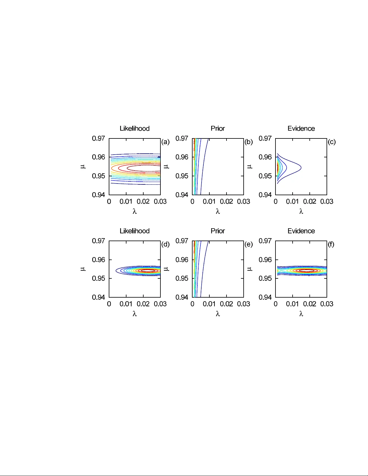
Applications of the Beta Distribution P art 1: T ransformation Group Approac h Rob ert W. Johnson 29 Stanebr o ok Ct., Jonesbor o, GA 30238 e-mail: robjohnson@alphawaveresearch.com Abstract: A transformation group approach to the prior for the param- eters of the beta distribution is suggested which accounts for finite sets of data by imposing a limit to the range of parameter v alues under consider- ation. The relationship b et ween the b eta distribution and the Poisson and gamma distributions in the contin uum is explored, with an emphasis on the decomposition of the model into separate estimates for size and shap e. Use of the b eta distribution in classification and prediction problems is discussed, and the effect of the prior on the analysis of some well known examples from statistical genetics is examined. Keyw ords and phrases: transformation group, Ba yesian inference, b eta distribution. 1. In tro duction The beta distribution of the first kind, usually written in terms of the incom- plete beta function, can b e used to model the distribution of measurements whose v alues all lie b etw een zero and one. It can also b e used to model the distribution for the probability of o ccurrence of some discrete even t. The most widely kno wn technique for estimating the parameters, the method of momen ts, simply selects that b eta distribution with the same first and second moments as found empirically from the data. Ho wev er, such a pro cedure is not well-justified from the p ersp ectiv e of probability theory . T o ev aluate the reliability of the es- timate of a mo del’s parameters, as w ell as to determine the net evidence for a particular model relativ e to some other, one needs to follo w the mathematical pro cedure which has come to be known as Bay esian data analysis. Use of the beta distribution can b e found in a v ariety of applications; for an ov erview of this and related classes of discrete statistical mo dels and their use in Ba yesian analysis, see Pereira and Stern ( 2008 ). One common use is as a mo del for an input process within a stochastic sim ulation ( Kuhl et al. , 2010 ). Another is in the calculation of costs exp ected from a civil or industrial engineering pro ject ( B¸ etk o w ski and Po wnuk , 2004 ). It also has widespread use in the study of p opulation genomics ( Balding and Nichols , 1995 ; Price et al. , 2006 ). This pap er concerns itself not so muc h with the c hoice of application but rather focuses on the methodology used to ev aluate the parameters of the model giv en a set of measuremen ts and the relativ e merit of competing models. V arious metho ds ha v e b een suggested for the estimation of its parameters, including the metho d of momen ts ( AbouRizk, Halpin and Wilson , 1991 ) and v ariants of the 1 R ob ert W. Johnson/Applications of the Beta Distribution Part 1 2 Kolmogoro v-Smirno v test ( Press et al. , 1992 ), as w ell as tests based on Ba yesian significance v alues ( Pereira, Stern and W echsler , 2008 ; Bernardo, Lauretto and Stern , 2012 ; Stern and Pereira , 2013 ). How ever, in this paper w e will follow the traditional approach based on Bay es factors expressed in terms of the joint distribution for the quantities of in terest. This pap er is organized as follo ws. After a brief description of Ba yesian data analysis, we explore the relation b etw een the b eta distribution and the Poisson and gamma distributions in the con tin uum. The join t densit y for the size and shap e parameter estimates can be expressed in alternate coordinate systems through geometric transformations whic h preserv e the v olume. Marginalization o v e r the size parameter leav es b ehind the b eta distribution which describ es the shap e (distributed occurrence of ev ents) of the possible outcomes. After that, w e examine the use of the beta distribution in the classification problem, where one tries to predict the t yp e of some new ob ject from the comparison of its features to those of a set of kno wn ob jects. The mo del is then applied to some w ell kno wn examples of genomic inference from population statistics of an observ able lo cus W e will conclude with a discussion of our findings and a summary of our results. Some readers may find our use of the transformation group approac h reac- tionary , archaic, or even naive, in ligh t of the voluminous literature discussing other, more complicated strategies for deriving the form of the prior given some mo del for the lik eliho o d of the observ ations, suc h as conjugate and entropic metho ds ( Raiffa and Schlaifer , 1961 ; Lazo and Rathie , 1978 ). Our resp onse is that the analysis of similarity transformations has a long history in ph ysics, leading one to statemen ts of conserv ation of energy and momentum resp ective to translations in time and space. When discussing the analysis of data, one should nev er forget that real measuremen ts carry an index for lo cation on the univ ersal manifold and are sub ject to the laws of nature; how m uch use is made of that information dep ends upon the application and the inv estigator. 2. Brief description of Ba yesian data analysis The Bay esian approach to data analysis is b est discussed using the language of conditional probability theory ( Bretthorst , 1988 ; Durrett , 1994 ; Sivia , 1996 ). The expression for “the probability of A giv en B” can be written most compactly as p ( A | B ) ≡ p A B , (1) where A and B can hav e arbitrary dimensionality; for example, A could b e a v ector of measuremen ts, and B could include b oth the vector of parameters asso ciated with some model as w ell as an y other conditioning statements suc h as the mo del index. The notation on the RHS of Equation ( 1 ) is more economical than that of the LHS in terms of both the amount of ink on the page and the amount of mental effort required to keep track of the distinction betw een prop ositional statements in the sup erscript and conditional statements in the subscript; it also helps main tain iden tification of the units of density , which R ob ert W. Johnson/Applications of the Beta Distribution Part 1 3 are carried b y the prop ositional statemen ts alone. The sum and pro duct rules of probabilit y theory yield the expressions for marginalization and Bay es’ theorem, p A = Z { B } dB p A,B , (2) p B A p A = p A B p B , (3) where marginalization follows from the requirement of unit normalization, and Ba y es’ theorem follows from requiring logical consistency of the joint densit y p A,B = p B ,A . Let us write as the vector m the parameters for some mo del M , and let the data be written as x . Bay es’ theorem then relates the evidence for the parameters given the data p m x to the likelihoo d of the data given the parameters p x m through the expression p m x ∝ p x m p m , (4) where the factor p m describ es the prior expectation o ver the parameter manifold in the absence of data, and the constan t of proportionality p x represen ts the c hance of measuring the data, whic h is usually reco vered from the normalization requiremen t of the evidence densit y R { m } d m p m x = 1. The essential feature of Ba yesian data analysis which tak es it beyond maxi- m um likelihoo d analysis is the inclusion of the prior density p m . The selection of the appropriate form of the prior for some coordinate mapping of the param- eter manifold is guided by the principle of indifference applied to the b ehavior of the mo del under similarit y transformations ( Jaynes , 1968 ; Sivia , 1996 ; Dose , 2003 ). Here, indifference is realized b y examining the transformation group of the parameter manifold giv en b y m . Having found the prior measure for one co ordinate system, the prior measure for alternate co ordinate systems can b e found through the use of a Jacobian transformation. When only one mo del is in play , its qualit y of fit is irrelev ant. If no other description of the data is a v ailable, the most one can do is fit the parameters for the mo del at hand. In order to accomplish the task of hypothesis testing, Ba y e sian data analysis forces one to sp ecify explicitly the alternatives. F or a set of mo dels indexed by M , the factors in Equation ( 4 ) must b e conditioned on the c hoice of M . F or t wo mo dels M ∈ { 1 , 2 } , the relative evidence is giv en b y the ratio of the net evidence for each mo del, ρ 1 | x 2 | x ≡ p 1 x p 2 x = p x 1 p 1 p x 2 p 2 , (5) where the factor p 1 /p 2 describ es any prior preference betw een the mo dels and usually is identified as unity . The factors in the likelihoo d ratio are giv en by the marginalization of the join t density ov er the parameter manifold for each mo del, p x M = Z { m } d m p x , m M = Z { m } d m p x m ,M p m M , (6) R ob ert W. Johnson/Applications of the Beta Distribution Part 1 4 where the use of prop erly normalized densities for the likelihoo d and prior is required. In particular, the prior p m is normalized to unit y ov er the parameter manifold while the likelihoo d p x m retains its physical normalization. An in teresting feature of Bay esian mo del selection is that it accoun ts natu- rally for Occam’s principle of efficiency . Assuming mo del 1 has some parameter a with uniform prior of exten t ∆ a , and taking the quadratic (Gaussian) approx- imation of its likelihoo d, without prior preference for either mo del the evidence ratio becomes p (1 | x ) p (2 | x ) = p ( x | a 0 , 1) p ( x | 2)  2 π δ 2 a ∆ 2 a  1 / 2 , (7) where a 0 is the optimum v alue of the parameter and δ 2 a is its v ariance. With an adjustable parameter, mo del 1 v ery likely pro vides a b etter quality of fit as measured b y the first ratio p ( x | a 0 , 1) /p ( x | 2); ho wev er, that is not the only factor in the net evidence ratio. The impro ved fit to the data comes at the cost of the Occam factor (2 π δ 2 a / ∆ 2 a ) 1 / 2 whic h measures the distribution of the evidence densit y relative to the parameter domain. One requiremen t for the Gaussian appro ximation is that the prior not sev erely restrict the lik eliho o d ∆ a  δ a , thus the Occam factor works against the p eak likelihoo d in the net evidence ratio in Equation ( 7 ). Another interesting feature is that, all else b eing equal, the mo del whose parameters ha ve the lar ger v ariance is the one preferred b y probability theory , as more of its parameter space is compatible with the measurements. Supp ose mo del 2 has its o wn parameter b with comparable domain ∆ b ≈ ∆ a and provides a comparable fit to the data p ( x | b 0 , 2) ≈ p ( x | a 0 , 1). In this case, the net evidence ratio reduces to p 1 x /p 2 x ≈ δ a /δ b , so that the net evidence for mo del 1 relative to 2 is given by the ratio of the deviation of their parameters. One criticism that is often lev eled at those who use Bay esian methods ( Gel- man , 2008 ) is that the “prior and p osterior [evidence] distributions represent sub jective states of kno wledge.” By w orking in the language of conditional prob- abilit y theory , what Bay esian metho ds require is that one specify the background kno wledge up on whic h an y inference of likelihoo d is based. F or example, one’s estimate of the lik eliho od of rain to day depends up on whether one has seen satellite images of clouds in the area. In v estigation of the transformation group asso ciated with the parameters in a mo del leads one to sp ecify the Haar mea- sure as the in trinsic density whic h can serve as an ob jectiv e prior in the absence of any further information. The existence and uniqueness of the Haar measure hold under very general conditions on the set of parameters considered. 3. Beta, P oisson, and gamma distributions in the contin uum The b eta distribution can be deriv ed from consideration of the P oisson and gamma distributions in the con tin uum ( Press et al. , 1992 ; Abramo witz and Stegun , 1964 ). Physically , a contin uum quantit y is understo o d to b e one for whic h the quantum unit is to o small to measure. Let us b egin by supp osing the amoun t A for some quantit y observ ed p er unit time is given b y a Poisson R ob ert W. Johnson/Applications of the Beta Distribution Part 1 5 pro cess with rate parameter a expressed in the same ph ysical units u a = u A , th us the likelihoo d can be written p A a = a A /e a Γ( A + 1) = a A /e a A Γ( A ) ≡ P oisson( A | a ) , (8) in terms of the gamma function Γ( A ). The discrete Poisson distribution is of course giv en by Γ( A + 1) → A ! for integer (quan tized) A , suc h that the sum o v er all A of the probability mass function is normalized, e − a P ∞ A =0 a A / A ! = 1. One should k eep in mind, how ever, that p A a is a probability density function whic h carries units of u − 1 A suc h that dA p A a is a pure num b er. The in tegral R ∞ 0 dA p A a cannot b e easily ev aluated; ho wev er, a collection of heuristic arguments (giv en in Appendix A ) indicate that its v alue also is unity . According to Jaynes ( 1968 ), the parameter for a P oisson pro cess m ust satisfy the same functional equation for transformations in scale as does the deviation parameter of a Gaussian distribution, thus the intrinsic (prior) densit y for a ∈ [0 , ∞ ] is given by p a = a − 1 / Z ∞ 0 da a − 1 ≡ a − 1 /C 0 , (9) whic h defines the infinite constan t C 0 . Note that C 0 is formally equal to the mass of a distribution with infinite extent and unit densit y , C 0 ≡ R ∞ −∞ dl for l = log a , th us it also app ears in the ubiquitous uniform prior of the maximum likelihoo d metho d. Readers who are uncomfortable with infinite normalization constan ts ma y instead consider C 0 ≡ lim  → 0 C  for C  ≡ R  −  dl , using equiv alen t limits suc h that symmetry with resp ect to scale is maintained. The in trinsic densit y p a , whose sole proposition is the existence of a , is recognized as the Haar measure for the group of p ositive real num b ers closed under the op eration of m ultiplication. Note that Jaynes’ expression for the prior differs by a p ow er from that obtained b y application of the Jeffreys procedure, defined in terms of the square ro ot of (the determinan t of ) the Fisher information (matrix). That pro cedure yields the prior p a F ∝ a − 1 / 2 when applied to the P oisson distribution. The Ja ynes prior is functionally inv ariant under transformations of the form α = ma n for given m and n , suc h that p α ∝ α − 1 , whereas p α F ∝ α (1 − 2 n ) / 2 n whic h is in v arian t only for n = 1. In the limit n → ∞ one finds p α F → p α , which can b e interpreted heuristically (but maybe not correctly) as follows. When ev aluating the Fisher information, the expectation v alue is taken o ver only a single datum, whereas the measuremen t pro cess could b e rep eated any num b er of times, which for the P oisson pro cess amoun ts to changing the unit of time. It seems, then, that the Ja ynes prior accoun ts for the p ossibility of an infinite num b er of measuremen ts when assigning the most general form of p a . The joint density ov er the manifold ( a, A ) can b e written as the pro duct of the conditional density p A a and in trinsic density p a , p a,A = p A a p a = a A − 1 /C 0 e a A Γ( A ) , (10) and its integral ov er a can b e ev aluated explicitly , Z ∞ 0 da p a,A = Z ∞ 0 da p A a p a = A − 1 /C 0 ≡ p A , (11) R ob ert W. Johnson/Applications of the Beta Distribution Part 1 6 whic h is recognized as the chance of measuring A . Ha ving equiv alen t physical units, the quantities a and A p ossess the same transformation group, thus their in trinsic densities must b e functionally iden tical. That the expression p a,A rep- resen ts a v alid probabilit y densit y function is v erified by next taking the in tegral o v e r A , Z ∞ 0 dA Z ∞ 0 da p a,A = Z ∞ 0 dA p A = 1 , (12) th us the joint densit y has unit mass o v er the infinite quarter plane [0 , ∞ ] × [0 , ∞ ] in R 2 . According to Ba y es’ theorem, the evidence for parameter a conditioned on observ able A in the P oisson likelihoo d is given by the gamma distribution, p a A = p A a p a /p A = a A − 1 /e a Γ( A ) ≡ Gamma( a | A ) , (13) whic h is normalized to unit mass, R ∞ 0 da p a A = 1. One also can v erify the in tegral R ∞ 0 da p A a = 1 (permissible since u a = u A ), thus the likelihoo d is normalized o v er the parameter a as well; logically , given the existence of a v alue for A , it m ust b e true that the sum of all its conditional probabilities is equal to unit y . By similar logic, the normalization of b oth p A a and p a A o v er A should also be true, but a direct ev aluation of those integrals analytically is difficult (see App endix A ). F or comparison, consider the joint density of a measurement M and parameter m giv en b y a Gaussian of known deviation whic h sets the scale, p m,M = exp[ − π ( M − m ) 2 ] /C 0 , with intrinsic densities p m = p M = 1 /C 0 . In this case, one can easily show that R ∞ −∞ dm p m M = R ∞ −∞ dm p M m = 1 as well as R ∞ −∞ dM p M m = R ∞ −∞ dM p m M = 1. That similar normalizations hold in the con tin uum for the Poisson and gamma densities is the main conjecture of this pap er. Note that the join t density p a,A do es not care whether a and A are iden tified as parameter and observ able, resp ectively , or vic e versa . The identification of evidence, chance, lik eliho od, and prior similarly is arbitrary , as long as one is consisten t ( Sivia , 1996 ). The decomposition through Ba y es’ theorem of the join t densit y in terms of in trinsic densities giv en b y the Haar measure allows one to write a − 1 P oisson( A | a ) = A − 1 Gamma( a | A ) , (14) th us the gamma distribution is the evidence for a Poisson process lik eliho o d, and vic e versa . The second (shap e) parameter commonly asso ciated with the gamma distribution can b e iden tified as the ratio of the units for the parameter and observ able u a /u A , whic h here is specified as unity . No w let us consider the join t density p a,b,A,B , whic h can b e written as p A,B a,b p a,b =  a A b B /e a + b AB Γ( A )Γ( B )  /abC 2 0 . (15) Under a change of co ordinate mapping ( a, b ) → ( x, y ) such that  x y  =  a/ ( a + b ) a + b  ⇐ ⇒  a b  =  xy (1 − x ) y  , (16) R ob ert W. Johnson/Applications of the Beta Distribution Part 1 7 with domain x ∈ [0 , 1] and y ∈ [0 , ∞ ], the Jacobian matrix is giv en by J a,b x,y ≡ ∂ ( a, b ) ∂ ( x, y ) =  y x − y 1 − x  , (17) whose determinant is | J a,b x,y | = y . The intrinsic densit y in the new co ordinates is th us p x,y = p a,b | J a,b x,y | = x − 1 (1 − x ) − 1 y − 1 /C 2 0 , (18) and the conditional density is p A,B x,y = x A (1 − x ) B y A + B /e y AB Γ( A )Γ( B ) . (19) Since p A,B = 1 / AB C 2 0 , one can then write p x,y A,B = p A,B x,y p x,y /p A,B = x A − 1 (1 − x ) B − 1 y A + B − 1 e − y / Γ( A )Γ( B ) , (20) whic h in tegrates to unit y , Z 1 0 dx Z ∞ 0 dy p x,y A,B = 1 , (21) using the ev aluations Z ∞ 0 dy y A + B − 1 e − y = Γ( A + B ) , (22) Z 1 0 dx x A − 1 (1 − x ) B − 1 = β ( A, B ) . (23) Marginalization then yields p x,A,B = Z ∞ 0 dy p x,y ,A,B = x A − 1 (1 − x ) B − 1 /β ( A, B ) AB C 2 0 (24a) = p x A,B p A,B , (24b) whic h is the main result of this section. With the interpretation of x = a/ ( a + b ) ∈ [0 , 1] as a normalized frequency (rate of observ ance), one can state that the in trinsic density for an absolute lik eliho o d is p x = x − 1 (1 − x ) − 1 /C 0 , while that for a relative lik eliho o d r = a/b ∈ [0 , ∞ ] is p r = r − 1 /C 0 . Note that C 0 is infinite only when the parameter is allo w ed to obtain the extreme v alues of its domain, and in fact is comprised of tw o indep endent infinities C 0 = 2 R ∞ 1 dr r − 1 , one from eac h b oundary of the manifold. While the relationship b et ween these three distributions has b een explored b y many authors, nowhere hav e w e found a deriv ation within the framework of conditional probabilit y theory that ties them together under the conjecture of the contin uum normalization. The literature has instead fo cused on the relation b et ween discrete random v ariables rather than the contin uous case. P artly that ma y b e because the expression of the Poisson distribution in the contin uum is R ob ert W. Johnson/Applications of the Beta Distribution Part 1 8 not so widely kno wn, o wing to the difficulty of ev aluating its normalization in- tegral analytically . Another reason may b e b ecause use of transformation group argumen ts has been championed primarily by physicists rather than statisti- cians. Whatev er the reason, the establishmen t of Equation ( 14 ) in the con tin- uum leads one naturally to the b eta distribution, which displa ys explicitly the transformation group prior for the normalized frequency x . Let us now consider the parametrization ( x, y ) → ( α, β ) given b y  α β  =  log y log x − log(1 − x )  ⇐ ⇒  x y  =  1 / [1 + e − β ] e α  , (25) with domain α, β ∈ [ −∞ , ∞ ]. In these co ordinates, the prior density is uniform p α,β = 1 /C 2 0 , thus the evidence is prop ortional to the likelihoo d, and the join t densit y equals p A,B α,β p α,β =  x A (1 − x ) B y A + B /e y AB Γ( A )Γ( B )  /x (1 − x ) y C 2 0 (26a) =  1 + e − β  − A  1 + e β  − B e ( A + B ) α { exp( e α ) AB Γ( A )Γ( B ) } − 1 /C 2 0 (26b) =  e α 1 + e − β  A  e α 1 + e β  B { exp( e α ) AB Γ( A )Γ( B ) } − 1 /C 2 0 (26c) =  e − α + e − α − β  − A  e − α + e − α + β  − B { exp( e α ) AB Γ( A )Γ( B ) } − 1 /C 2 0 . (26d) The first t w o factors abov e are reminiscent of the logistic regression mo del ( P eng and So , 2002 ); how ever, the parameter α , commonly called “the in tercept”, mak es an appearance as the argumen t of a double exp onential in the third factor as well as in the terms e − α without β . The third factor is not related to the prior thus must b e part of the likelihoo d. Rather than conflating the parameters, keeping the likelihoo d mo dels p A,B α ∝ e ( A + B ) α / exp e α and p A,B β ∝ [1 + e − β ] − A [1 + e β ] − B indep enden t leads to a more efficien t ev aluation ( Johnson , 2017 ). 4. Application to prediction and classification Let us b egin this section b y talking ab out baseball. Sp ecifically , let us consider the use of the seasonal batting av erage as a predictor for whether a play er will reac h base on his next app earance. Let eac h app earance b e indexed by time giv en by integer t ∈ [1 , T ], and let us identify a successful app earance as an ev en t of type A , while outs are of type B . The record of successful app earances can b e notated by A ≡ A j for j ∈ [1 , J ], and similarly for B ≡ B k of dimension K , suc h that T = J + K . The evidence for the v alue of the batting a verage x is the pro duct of the prior and likelihoo d factors, yielding the b eta distribution p x J,K ∝ x J − 1 (1 − x ) K − 1 with mode x E = ( J − 1) / ( J + K − 2) and exp ectation v alue h x i x | J,K = J / ( J + K ), which coincides with the lik eliho o d mo de x L and giv es the predicted rate of success for the next appearance. One can incorporate in to the form of the prior p x additional information p ertinen t to the problem at hand. In particular, one can use kno wledge of the R ob ert W. Johnson/Applications of the Beta Distribution Part 1 9 seasonal nature of the sp ort to impose sensible limits on the domain x ∈ [ , 1 −  ]. If our pla yer’s season is not y et o ver, then there m ust b e at least one more at bat sc heduled. A sensible limit is thus given by  = 1 / ( T + 1), which incorp orates the notions that nobo dy is p erfect (1 is excluded) and of the benefit of the doubt (0 is excluded); assuming our play er is a professional at least one even t of eac h type should b e observed p er season, ev en for pitchers. One effect of such a prior is that it do es not allow observ ations of only one type of ev ent to pull the evidence mo de all the wa y to the h yp othetical limits of 0 and 1. Another effect is that early in the season T & 1 the domain of x requires an observ ation of the batter b efore starting to make predictions; once we are certain the batter is pla ying this season T = 1, we can state the exp ected chance of success is equal to 1/2, the only allow ed p oint, with further observ ations expanding the domain un til at the end of a long season T  1 the prior is wide open. Let us no w turn to consideration of classifying some new even t as type A or B on the basis of its lo cation relative to those for T observ ations whose classification is assigned. The elemen ts of the measuremen t vectors A and B are now locations along some axis τ , with a measurement uncertaint y expressed b y the Gaussian deviation σ . If the chance an even t is of type A is indep endent of lo cation, one can write p x,τ σ, A , B ∝ p x J,K p τ σ, A , B , where p τ σ, A , B is a Gaussian cen tered on the mean lo cation of all the even ts and each margin is normalized indep enden tly . That is ob viously not the solution w e are lo oking for, whic h should giv e an exp ectation of the form x ( τ ) based on a joint density that can b e factored as p x,τ σ, A , B = p x σ,τ, A , B p τ for p τ ∝ 1. Another wa y to express the notion that lo cation has become irrelev ant is b y taking the limit σ → ∞ . In that case, one should require p x σ,τ, A , B → p x J,K for all τ , whic h corresp onds to neglecting the stadium of app earance in the batting a v erage problem ab o v e. In doing so, w e ha ve not said that lo cation do es not exist, but rather that lo cation do es not matter. F or finite σ , w e should write p x σ,τ, A , B ∝ p x p A , B σ,τ,x , whose limit for τ → ∞ is p x ; observ ations nearb y should not significan tly affect our prediction for a galaxy far, far aw ay . The problem now is one of assigning the appropriate form for the likelihoo d factor. F or inspiration, w e hav e lo oked at v arious approaches suggested in the literature ( T errell and Scott , 1992 ; Hall, Park and Samw orth , 2008 ; Kim and Scott , 2012 ; Eb erts and Stein w art , 2013 ). A t this stage the discussion b ecomes a bit heuristic. When the observ ations are independent, we can factor the lik eliho o d in to the form p A , B σ,τ,x = Y j p j σ,τ,x Y k p k σ,τ,x , (27) where p j σ,τ,x represen ts the chance datum j is of t yp e A , and s imilarly for p k σ,τ,x . What, then, is the form of p j σ,τ,x that yields sensible results for all σ and ir- resp ectiv e of the underlying spatial distributions of the t wo types of even ts? A form which suggests itself is more clearly notated in terms of its logarithm q j σ,τ,x = − r j τ log x , where r j τ = exp − 1 / 2 [( A j − τ ) 2 /σ 2 ] is the probability of an ev en t at A j relativ e to that at τ . The log of the likelihoo d can then be written R ob ert W. Johnson/Applications of the Beta Distribution Part 1 10 Fig 1 . Distributions A ( τ ) and B ( τ ) as describ e d in the text. The lo c ations A j ar e indic ate d at the top of e ach plot, and B k ar e at the b ottom. as − q A , B σ,τ,x = X j r j τ log x + X k r k τ log(1 − x ) , (28) whose limits are J log x + K log(1 − x ) for σ → ∞ and 0 for τ → ∞ , in accord with our requiremen ts for the evidence density . Let us iden tify A ( τ ) ≡ P j r j τ , and similarly for B ( τ ); then the likelihoo d can be written as x A ( τ ) (1 − x ) B ( τ ) , and the evidence for the v alue x at τ is given by p x σ,τ, A , B ∝ x A ( τ ) − 1 (1 − x ) B ( τ ) − 1 , (29) whic h has the form of a b eta distribution at all locations. An example of A ( τ ) and B ( τ ) for an arbitrary distribution of A and B in units of the deviation σ = 1 is shown in panel (a) of Figure 1 . The v alues A j are dra wn uniformly o v er tw o disjoin t regions each with a span of 2 units, and the v alues B k are selected from a region spanning 2 units which ov erlaps partially one of the t yp e A regions. Out of resp ect for our heuristic argumen t, w e should consider some alternative definitions for the lik eliho o d. If instead of the relative probabilities r j τ one defines A ( τ ) as the sum of the absolute probabilities p j σ,τ = (2 π σ 2 ) − 1 / 2 r j τ suc h that R dτ P j p j σ,τ = J , one has in the limit σ → ∞ the result A ( τ ) → 0, which do es not reco ver the beta distribution in terms of J and K . If one uses the pro duct of the datum lik eliho o ds to define A ( τ ) = J (2 πσ 2 /J ) − 1 / 2 exp − 1 / 2 [( τ − µ A ) 2 J /σ 2 ] for µ A = h A j i j , which also integrates ov er τ to J , one’s estimate for the evidence dep ends up on only the first moments of the even t distributions, a procedure which is easily foiled when the underlying location distribution are not Gaussian. Finally , if one uses p j σ,τ,x = xp j σ,τ , one recov ers simply the R ob ert W. Johnson/Applications of the Beta Distribution Part 1 11 Fig 2 . Pr e diction values x ( τ ) fr om A ( τ ) and B ( τ ) as describ e d in the text. The maximum likeliho o d pre dictor x ML is shown as  , and the exp e ctation value x EV is shown as ♦ . indep enden t distributions ov er x and τ . Examples of these definitions of A ( τ ) and B ( τ ) are display ed in panels (b) through (d) resp ectiv ely of Figure 1 for the same distributions of A j and B k . A maxim um likelihoo d predictor can b e formed from the expression x ML ( τ ) = [1 + B ( τ ) / A ( τ )] − 1 , (30) whic h is ev aluated from the measuremen ts A and B with resp ect to σ . The exp ectation v alue x EV ( τ ) = h x i x | σ,τ, A , B , how ever, tak es into accoun t the full domain of x as measured b y the evidence density . In Figure 2 we display the maxim um lik eliho od and exp ected v alue predictors for the distributions A ( τ ) and B ( τ ) shown in Figure 1 . The lik eliho o d estimate x ML is the same in panels (a) and (b), since the ratio B ( τ ) / A ( τ ) in terms of the summed likelihoo ds does not dep end on their normalization. The exp ectation v alue in panel (b) is more conserv ativ e, in that it more quickly approaches the exp ectation v alue of the prior, compared to panel (a). The lik eliho o d estimate for the metho d of panel (c) giv es a prediction for the region τ ∈ [ − 2 , − 1] that is con trary to the observ ations, while its exp ectation v alue is v ery quickly drawn to that of the prior, even in the region τ > 1 . 5 where only t yp e A ev ents are observ ed. The lik eliho od and exp ectation v alue predictors are identical when the lo cation information is ignored, as seen in panel (d). Let us now rep eat the ev aluation of the evidence densities p x σ,τ, A , B for the v arious definitions of A ( τ ) and B ( τ ), but this time let us suppose that σ = 10 for the same locations A and B . Let us also insp ect the evidence densities directly , to see which one best enco des a reasonable estimate of the solution to our problem. In Figure 3 w e displa y the evidence densit y for x as a function of τ for the v arious lik eliho o d models. W e can see that panel (a) is the one most R ob ert W. Johnson/Applications of the Beta Distribution Part 1 12 Fig 3 . Evidence densities p x σ,τ, A , B for σ = 10 as describ ed in the text. lik e panel (d), which ev aluates the b eta distribution without regard to lo cation. The other mo dels, panels (b) and (c), are not in accord with the conclusions a reasonable observ er w ould dra w in tuitively from the presen ted data; surely with close to 100 observ ations the relative rate of pro duction should b e fairly w ell determined o ver the common region of the ev ents. While our justification of Equation ( 28 ) is heuristic, its form is the same as that of a Gaussian with unequal w eigh ts , where each datum factor in the lik eliho od is an absolute probability to the pow er of a relativ e probability . What can w e sa y about the limit σ → 0, whic h indicates that observ ations are relev an t only to predictions at the same lo cation? With resp ect to the finite res- olution of whatev er apparatus is used to tak e the lo cation measuremen ts, what w e really mean in that limit is that locations are resolved o v er a set of discrete c hannels whic h ha v e no influence or bearing on even ts in other c hannels. Return- ing to the baseball analogy , that mo del asserts that batting av erages for each stadium should b e ev aluated indep enden tly , which is not an unreasonable pro ce- dure, given by A ( τ ) = P A ( j )= τ r j τ and similarly for B ( τ ). The parameter τ can in fact b e an abstract location, not just a ph ysical one, with the in terpretation of r j τ as the relev ance of observ ations in one channel to predictions in another. W e should also p oint out that we hav e been treating the lo cation τ of the predicted classification as a quantit y kno wn exactly; if the location of the unclassified even t τ 0 is itself sub ject to measuremen t deviation σ , then one must con v olute the ev- idence density with its normalized distribution, p x σ,τ 0 , A , B = R dτ p τ σ,τ 0 p x σ,τ, A , B . F urthermore, if the v alue of σ is unknown, it can b e integrated out by treating it as as a n uisance parameter, p x τ 0 , A , B = R dσ p σ p x σ,τ 0 , A , B for p σ ∝ σ − 1 . R ob ert W. Johnson/Applications of the Beta Distribution Part 1 13 5. Application to the Balding-Nic hols mo del Next let us look at how the beta distribution is used in the analysis of genetic profiles. Supp ose the gene at some lo cus has a dominant allele G and a recessive allele g such that the genotypes GG , Gg , and g g are distinguishable. According to Balding and Nichols ( 1995 ), the allele frequency x for finding G at the lo cus follo ws a beta distribution with parameters A = µ (1 − λ ) /λ and B = (1 − µ )(1 − λ ) /λ . The measuremen ts are no w not v alues for x k but rather the num b er of mem b ers of each genotype observed within a sampling of the k th p opulation, N k = N k,GG + N k,Gg + N k,g g . In terms of the parameters, the probability for an individual to b e a member of the genot yp e is given b y p GG A,B ≡ h x 2 i x | A,B = A ( A + 1) / ( A + B )( A + B + 1) (31a) = λµ + (1 − λ ) µ 2 (31b) for the dominant homozygote, and b y p g g A,B ≡ h (1 − x ) 2 i x | A,B = B ( B + 1) / ( A + B )( A + B + 1) (32a) = λ (1 − µ ) + (1 − λ )(1 − µ ) 2 (32b) for the recessive homozygote, while the heterozygote app ears with probabilit y p Gg A,B ≡ 2 h x (1 − x ) i x | A,B = 2 AB / ( A + B )( A + B + 1) (33a) = 2(1 − λ ) µ (1 − µ ) , (33b) where the factor of 2 accounts for the indistinguishability of the order of the alleles. In matrix form with unit 1-norm, the joint distribution of the genotypes can be written " p GG λ,µ p Gg λ,µ / 2 p Gg λ,µ / 2 p g g λ,µ # = λ  µ 0 0 1 − µ  + (1 − λ )  µ 2 µ (1 − µ ) µ (1 − µ ) (1 − µ ) 2  , (34) yielding the interpretation of µ = (1 + B / A ) − 1 as the mean dominant allele frequency and of λ = (1 + A + B ) − 1 as a measure of heterozygote suppression. The parameter λ may b e iden tified with W righ t’s in breeding co efficient F . The probability of obtaining the measurements giv en kno wledge of the param- eter v alues is the pro duct of the genot yp e likelihoo ds weigh ted by the n umber of mem b ers. F or a single p opulation, p N GG ,N Gg ,N gg A,B = ( p GG A,B ) N GG ( p Gg A,B ) N Gg ( p g g A,B ) N gg , (35) th us the information conten t of the data (negative log lik eliho o d) is L ( A, B ) ≡ q N GG ,N Gg ,N gg A,B = N GG q GG A,B + N Gg q Gg A,B + N g g q g g A,B , (36) recalling q ≡ − log p . The non trivial solution of ∇ L ( A, B ) = 0 yields the maxi- m um lik eliho o d estimate of the optimal parameter v alues  a L b L  =  (2 N Gg N GG + N 2 Gg ) / (4 N GG N g g − N 2 Gg ) (2 N Gg N g g + N 2 Gg ) / (4 N GG N g g − N 2 Gg )  , (37) R ob ert W. Johnson/Applications of the Beta Distribution Part 1 14 whic h corresponds to the location  λ L µ L  =  (4 N GG N g g − N 2 Gg ) / [(2 N g g + N Gg )(2 N GG + N Gg )] (2 N GG + N Gg ) / 2( N GG + N Gg + N g g )  (38) on the ( λ, µ ) manifold. Supp ose now instead of the genotype observ ations our data consists of the ra w allele counts for G and g , giv en by N G ≡ 2 N GG + N Gg and N g ≡ 2 N g g + N Gg suc h that 2 N = N G + N g . The log likelihoo d in this case b ecomes q N G ,N g A,B = N G log(1 + B / A ) + N g log(1 + A/B ) (39a) = − N G log µ − N g log(1 − µ ) , (39b) whose optimal estimate is the same µ L = (1 + N g / N G ) − 1 with λ undetermined. F rom the ra w allele coun ts one can resolve only the dominan t allele frequency for a single p opulation. The merit function for the evidence densit y p λ,µ N GG ,N Gg ,N gg in terms of the parameters ( λ, µ ) can b e written as F ( λ, µ ) = L ( λ, µ ) + log [ λ (1 − λ ) µ (1 − µ )] , (40) using an unnormalized prior. When λ = 0, the p opulation is said to be in Hardy–W einberg equilibrium with a single parameter µ for the dominant allele frequency; how ever, one should observe that λ = 1 is also an equilibrium solution with a single parameter µ . Those t w o cases corresp ond to the p eaks in the prior for λ when the b oundary is not excluded. In the limit  → 0, the normalized prior p λ has the v alue 1/2 at λ equal to 0 or 1 and the v alue 0 everywhere else. Similarly , when µ equals 0 or 1, one finds that λ is undetermined by the lik eliho od, thus those mo dels ha v e zero free parameters. The fiv e mo dels under consideration (for a single p opulation) can th us b e lab eled M λ,µ , M 0 ,µ , M 1 ,µ , M 0 , and M 1 , where the first is a tw o parameter model, the next tw o are one parameter models, and the last tw o zero parameter mo dels, all of whic h are conditioned on the v alue of the b oundary exclusion  determined in principle by the nature of the measurement apparatus. A similar approac h is suggested b y Johnson and Rossell ( 2010 ). See Figure 4 for a depiction of the mapping from the parameter manifold to the model lab els using a large v alue of  for clarity . It is instructive to look at the information con tent of the data with resp ect to the v arious mo dels. F or M λ,µ with t w o parameters, L λ,µ is giv en b y Equa- tion ( 36 ), whose mo de pro vides a go o d starting p oint for the n umerical optimiza- tion of F λ,µ ; four other p oints to consider are the pro jections of the lik eliho o d mo de on to the b oundaries of the manifold. The mo del M 0 ,µ has an information densit y of L 0 ,µ ( µ ) = − N Gg log 2 − (2 N GG + N Gg ) log µ − (2 N g g + N Gg ) log(1 − µ ) , (41) retaining the constant term with N Gg , and M 1 ,µ has L 1 ,µ ( µ ) = − N Gg log 0 − N GG log µ − N g g log(1 − µ ) , (42) R ob ert W. Johnson/Applications of the Beta Distribution Part 1 15 Fig 4 . Mapping fr om the p arameter manifold ( λ, µ ) to the model labels describe d in the text for an exagger ate d value of  . T able 1 Genotyp e observations fr om F or d ( 1971 ) and maximum likeliho o d r esults with values for λ , µ , and P state d in units of per c ent N GG N Gg N gg λ L µ L χ 2 P P 1 ( χ 2 P ) 1469 138 5 2.270 95.409 0.831 63.8 supp orted only when N Gg = 0 such that N Gg log p Gg λ =1 = log 0 0 = 0; otherwise, L 1 ,µ = ∞ . F or either one parameter model, it is p ossible for certain v alues of the input data to yield an evidence densit y which is uniform in µ ; in those cases, the mo de is undetermined and the unnormalized evidence density is equal to 1. F or the zero parameter models, L 0 = − N GG log 0 − N Gg log 0 − N g g log 1 , (43) whic h equals 0 when only N g g > 0 else is infinite, and b y symmetry L 1 = − N GG log 1 − N Gg log 0 − N g g log 0 . (44) Since the zero parameter mo dels hav e a manifold of a single p oint, their net evidence (mean likelihoo d) is either 0 or 1 according to whether they are sup- p orted by the data, whic h sets the unit of evidence when comparing the other mo dels. As an illustration, let us lo ok first at some data from F ord ( 1971 ) shown in T able 1 . Also shown are the maxim um likelihoo d v alues λ L and µ L in units of p ercen t. F rom these num b ers one can ev aluate P earson’s statistic χ 2 P from the Hardy–W einberg exp ectation v alues N H W GG = N µ 2 L and so on. The accum ulation of the χ 2 P statistic for 1 degree of freedom (3 from the data less 2 used in the mo del) gives the significance P 1 ( χ 2 P ) of the deviation from equilibrium, and for comparison P 1 (3 . 84) ≈ 95% for P d ( χ 2 ) ≡ γ ( d/ 2 , χ 2 / 2) / Γ( d/ 2) in the notation used by Press et al. ( 1992 ). The conv entional in terpretation is to state that R ob ert W. Johnson/Applications of the Beta Distribution Part 1 16 T able 2 Evidenc e analysis of the data fr om T able 1 with values for λ , µ , and Q stated in units of p er cent model: λ, µ 0 , µ 1 , µ 0 1 mode: (0.001,95.438) 95.438 NaN NaN NaN mean: (0.985,95.407) 95.409 NaN NaN NaN q M N : 510.4 509.6 Inf Inf Inf Q M N : 30.2 69.8 0.0 0.0 0.0 the equilibrium mo del is not rejected on accoun t of the small v alue of χ 2 P ; ho w e v er, since only tw o models are considered, one ma y in terpret the v alue of P 1 ( χ 2 P ) as the amoun t of probability not assigned to the equilibrium model, in whic h case the maxim um lik eliho o d analysis is sho wing some preference, if not o v e rwhelming, for the non-equilibrium model. The evidence analysis of the same data is shown in T able 2 for all five mo dels. A v alue of  = 10 − 5 is selected, consistent with the amount of data N GG + N Gg + N g g = 1612; in other w ords, w e select a mathematical resolution sligh tly b ey ond that giv en b y the measurement pro cedure whic h excludes the extreme b oundary . The location of the mode, when it exists, is displa yed, as are the exp ected v alues of the parameters; for mo del M λ,µ the global optimum of evidence is lo cated on the b oundary , and for mo del M 0 ,µ the mean v alue for µ is equal to µ L as exp ected analytically . The net evidence for eac h model M is giv en in terms of its negativ e logarithm q M N ≡ − log h p N m i m for parameter v ector m and data v ector N ≡ ( N GG , N Gg , N g g ). The Q v alue for each mo del, in terpreted as the probabilit y that the mo del describes the data, is determined from Q M N ≡ exp( − q M N ) / X M exp( − q M N ) , (45) suc h that P M Q M N = 1. Of the tw o mo dels supp orted by the data, that for Hardy–W einberg equilibrium M 0 ,µ is assigned a probability close to 70%. A graphical comparison of the lik eliho o d and evidence analysis is sho wn in Figure 5 panels (a)–(c); in panels (d)–(f ) we show the analysis of a hypothetical data set with 10 times as man y observ ations per channel at the same ratios. With that m uc h data, the evidence is mostly around the likelihoo d p eak, but a noticeable fraction is left along the manifold b oundary . F or the amoun ts of data commonly found in observ ational studies, the prior can hav e a significan t effect on the analysis. Next let us lo ok at some data from James et al. ( 1983 ) as summarized by Holsinger ( 2006 ), displa y ed in T able 3 . This time the data is broken do wn into that for subpopulations indexed b y k according to the geographic region of the observ ations. Since none of the populations ha v e only N g g > 0, the mo del M 0 can be discarded immediately . The practical question w e are interested in is whether any single p opulation is significantly differen t than the remainder. T o answer that question, the net evidence (expected likelihoo d) for the models applied to the en tire p opulation N 0 ≡ P k N k is compared to the product of the evidence for the sub division into N k and N ∼ k ≡ N 0 − N k . The results of this R ob ert W. Johnson/Applications of the Beta Distribution Part 1 17 Fig 5 . Comp arison of the likeliho od, prior, and evidence densities in the analysis of data fr om T able 1 in p anels (a)–(c); for panels (d)–(f ) the data is multiplie d by a factor of 10. R ob ert W. Johnson/Applications of the Beta Distribution Part 1 18 T able 3 Genotyp e observations fr om James et al. ( 1983 ) k 1 2 3 4 5 6 7 8 9 10 11 12 N GG 29 14 15 9 9 23 23 29 5 1 0 1 N Gg 0 3 2 0 0 5 3 3 0 0 1 0 N gg 0 3 3 0 0 2 4 1 0 0 0 0 T able 4 Evidenc e analysis in terms of mo des, means, and q values of the data fr om T able 3 for the entir e p opulation N 0 , the subp opulations N k indexe d by k , and the r emainder p opulations N ∼ k indexe d by k k λ λ,µ µ λ,µ µ 0 ,µ µ 1 ,µ h λ i λ,µ h µ i λ,µ h µ i 0 ,µ h µ i 1 ,µ q λ,µ q 0 ,µ q 1 ,µ q 1 0 0.55 0.89 0.89 NaN 0.55 0.89 0.89 NaN 110.05 125.93 Inf Inf 1 1.00 1.00 1.00 1.00 0.52 1.00 1.00 1.00 1.16 1.21 1.11 0.00 2 0.00 0.79 0.79 NaN 0.45 0.77 0.78 NaN 21.41 22.43 Inf Inf 3 0.00 0.82 0.82 NaN 0.62 0.80 0.80 NaN 19.62 21.76 Inf Inf 4 1.00 1.00 1.00 1.00 0.52 0.99 0.99 0.99 1.01 1.05 0.96 0.00 5 1.00 1.00 1.00 1.00 0.52 0.99 0.99 0.99 1.01 1.05 0.96 0.00 6 0.00 0.86 0.86 NaN 0.19 0.85 0.85 NaN 25.19 25.12 Inf Inf 7 0.00 0.83 0.83 NaN 0.63 0.82 0.82 NaN 26.51 29.81 Inf Inf 8 0.00 0.94 0.94 NaN 0.20 0.92 0.92 NaN 18.69 18.59 Inf Inf 9 1.00 1.00 1.00 1.00 0.52 0.98 0.99 0.98 0.93 0.98 0.89 0.00 10 1.00 1.00 1.00 1.00 0.52 0.93 0.95 0.91 0.74 0.78 0.69 0.00 11 0.00 0.50 NaN NaN 0.18 0.50 0.50 NaN 3.85 3.14 Inf Inf 12 1.00 1.00 1.00 1.00 0.52 0.93 0.95 0.91 0.74 0.78 0.69 0.00 1 0.54 0.87 0.87 NaN 0.53 0.86 0.86 NaN 104.50 118.23 Inf Inf 2 0.54 0.90 0.90 NaN 0.53 0.90 0.90 NaN 91.97 104.33 Inf Inf 3 0.52 0.90 0.90 NaN 0.51 0.90 0.90 NaN 94.29 105.81 Inf Inf 4 0.55 0.88 0.88 NaN 0.54 0.88 0.88 NaN 108.43 123.69 Inf Inf 5 0.55 0.88 0.88 NaN 0.54 0.88 0.88 NaN 108.43 123.69 Inf Inf 6 0.61 0.90 0.89 NaN 0.60 0.89 0.89 NaN 88.24 103.50 Inf Inf 7 0.51 0.90 0.90 NaN 0.50 0.90 0.90 NaN 87.66 97.79 Inf Inf 8 0.58 0.88 0.88 NaN 0.57 0.88 0.88 NaN 94.90 109.60 Inf Inf 9 0.55 0.89 0.88 NaN 0.54 0.88 0.88 NaN 109.16 124.70 Inf Inf 10 0.55 0.89 0.89 NaN 0.55 0.89 0.89 NaN 109.87 125.69 Inf Inf 11 0.57 0.89 0.89 NaN 0.56 0.89 0.89 NaN 107.59 124.32 Inf Inf 12 0.55 0.89 0.89 NaN 0.55 0.89 0.89 NaN 109.87 125.69 Inf Inf analysis are sho wn in T able 4 using a v alue of  = 10 − 5 . V alues of 0 or 1 for the parameter mo de app earing in the table are understoo d to be on the b oundary giv en b y  . T o iden tify which single p opulation displays the most significan t deviation from the remainder, for eac h k the minim um q M N k is added to the minim um q M N ∼ k , then the minim um q M N 0 is subtracted to yield the (negative) log evidence for the sub division relative to the net population q k 0 . Those v alues are then exp onen tiated and normalized to yield the quality factors Q k 0 . F rom T able 4 one sees that M λ,µ is the model b est supp orted b y the net population and all the remainder p opulations, but all four mo dels can b e supported b y some of the subp opulations N k . In T able 5 we display which mo del M k b est fits p opulation N k as well as the relative log evidence q k 0 and the quality factors Q k 0 in units of percent. Of the thirteen mo dels under comparison, the most significan t is R ob ert W. Johnson/Applications of the Beta Distribution Part 1 19 T able 5 Evidenc e c omparison for the division of the data fr om T able 3 into subp opulations of N k and N ∼ k r elative to the entir e population N 0 with Q state d in units of p er c ent k 0 1 2 3 4 5 6 7 8 9 10 11 12 M k λ, µ 1 λ, µ λ, µ 1 1 0 , µ λ, µ 0 , µ 1 1 0 , µ 1 q k 0 0.00 -5.55 3.33 3.87 -1.61 -1.61 3.31 4.13 3.45 -0.89 -0.18 0.68 -0.18 Q k 0 0.37 93.96 0.01 0.01 1.84 1.84 0.01 0.01 0.01 0.89 0.44 0.18 0.44 the sub division of the first p opulation k = 1 from the remainder, whose Q is close to 94%. The suppression of the recessive allele in that p opulation would app ear to b e significan t, while that for the other p opulations displaying only N GG > 0 is less so. A thorough analysis would consider all possible groupings of the subp opulations to determine the most statistically significant division of the net p opulation from the given data. A more thorough analysis would mak e use of kno wledge of the geographical regions sampled to consider only those groupings of populations in physical contact. The p ossibilities are endless and left as an exercise for the reader. 6. Discussion and conclusion Those who use Bay esian metho ds are often asked to explain the significance of the prior. On its own, Bay es’ theorem do es not tell one how to assign the in trinsic probabilit y densit y for the parameter manifold. F or that task, one m ust turn to some other maxim. The principle of indifference is essen tially a geometric argumen t that p osits the existence of some co ordinate mapping of the parameter manifold for whic h the information con tent is uniform. That mapping migh t not b e the one most conv enient for the in vestigator, thus the appearance of the pri or ma y b e non uniform in one’s chosen co ordinates. The main effect of the prior is to prev en t one from o verestimating structure in the mo del not supported by imp erfect data. If the prior is neglected, one may uninten tionally in tro duce a bias in to one’s results. With respect to the b eta distribution, use of the transformation group prior is implicit in its functional form. In the absence of observ ations, what remains is the Haldane prior p x ∝ x − 1 (1 − x ) − 1 expressing complete indifference to the v alue of an absolute probabilit y . If the observ ations A and B are restricted to in teger coun ts of class membership, then the effect of the prior is to require an observ ation of each t yp e of even t b efore one is certain b oth types are present within the p opulation; until both t yp es ha ve b een observ ed, the evidence densit y is infinite on the b oundary at either 0 or 1. If one of each type has b een observ ed, w e are then certain that the pro duction rate x is b etw een 0 and 1 with uniform distribution. F urther observ ations then refine that estimate un til the likelihoo d and evidence mo des conv erge in the limit of infinite data. The transformation group approach leads one to specify q A,B = log A + log B as the logarithm of the unnormalized prior measure ov er the ( A, B ) manifold. In the course of this pro ject we inv estigated use of the entropic prior p A,B ∝ R ob ert W. Johnson/Applications of the Beta Distribution Part 1 20 exp( h q x A,B i x | A,B ), where − q A,B = log β ( A, B ) + ( A + B − 2)Λ 1 ( A + B ) + (1 − A )Λ 1 ( A ) + (1 − B )Λ 1 ( B ) (46) is ev aluated from the Shannon-Jaynes expression ( Lazo and Rathie , 1978 ). The en tropic expression for the prior was discarded after finding in the con text of the Balding-Nic hols genotype analysis that it did not lead to a hierarch y of mo dels. The Jeffreys inv ariant prior, with logarithm − q A,B = 2 − 1 log { Λ 2 ( A )Λ 2 ( B ) − [Λ 2 ( A ) + Λ 2 ( B )]Λ 2 ( A + B ) } (47) and prop ortional to the square ro ot of the determinant of the Fisher matrix, lik ewise w as considered. Its prior density is very similar to that given by the transformation group, thus results based on that prior should b e close to the results presen ted here. Finally , the conjugate prior approac h is discoun ted b e- cause there is no physical reason to supp ose that the evidence and prior should b e of the same algebraic form, mathematical con venience not withstanding. Note that the appearance of the b eta function in the b eta distribution results from the normalization ov er the axis x ∈ [0 , 1]; if the domain of x is more restrictive, the expression for the normalization as a function of the parameters A and B is more complicated. In that case, neither the en tropic nor the Jeffreys prior is appropriate without severe modification, whereas the transformation group prior is unaltered. Man y in vestigators are troubled b y the use of an improper prior, leading to an en tire industry devoted to the generation of ever more complicated functions to b e used as priors for statistical analysis of data. One should think very carefully b efore deciding to emplo y an y of those alternativ e strategies. Stern ( 2011 ) argues that go o d choices for the functional form of the probability densities used in a statistical mo del m ust b e based on the natural symmetries and inv ariance prop erties of the quan tities of in terest. The transformation group approach is based on the physical prop erties of the ob jects under consideration, with resp ect to the nature of the universe that we live in. The prior it yields represents a measure of uniform information conten t ov er the parameter manifold. The one dimensional improper transformation group priors are in fact all just different views of the uniform prior under a change of co ordinates, R 1 0 dx/x (1 − x ) = R ∞ 0 dz /z = R ∞ −∞ du for u = log z and z = x/ (1 − x ). The app earance of infinite densities on the b oundary of the prior indicate where simpler mo dels with fewer parameters exist; these models can b e addressed b y ev aluating their Bay es factor relativ e to the mo del with the most complexity . An outstanding issue when using the transformation group approach is the imp osition of the finite cutoff  . In the realm of physics, one argues that the measuremen t apparatus has a finite domain of resolution, from whic h a s ensible v alue of  may b e deriv ed. Practically , one often sets  to some v alue w ell b ey ond the expected domain of resolution with the understanding that one should c heck for b oundary effects, and for many problems with w ell resolved parameters that is sufficient. F or counting exp erimen ts with a P oisson likelihoo d, the total n um- b er of observ ations is constrained b y the patience of the inv estigator, thus it R ob ert W. Johnson/Applications of the Beta Distribution Part 1 21 pro vides a finite limit to the resolution. The sharp cutoff at  , though, is not app ealing, when intuitiv ely one exp ects a prop er prior with finite normalization to ha ve a smo oth b eha vior. F orthcoming in Part 2 is an extension of the ap- proac h presented here that incorp orates depth of data in a manner that yields a smo oth, normalizable prior function whose domain extends to the b oundaries. In summary , we hav e explored the relation b et ween the Poisson and gamma distributions in the contin uum with respect to the transformation group prior whose marginalization yields the beta distribution. T o impose normalization on the prior, we consider the limit on resolution of the parameters given by a finite set of observ ations. Some examples of the approach are presented which displa y the flexibilit y of the b eta distribution to model observ ational exp eriments. Its study has a long history in the literature, and it contin ues to b e quite useful in the modern day . APPENDIX A. Normalization of the con tinuum P oisson distribution In Section 3 we encountered an integral that could not b e put in to closed form analytically . In this app endix w e presen t some heuristic arguments for its ev al- uation. Let I ( a ) ≡ Z ∞ 0 dA a A Γ( A + 1) = Z ∞ 0 dA a A A Γ( A ) (48) represen t the integral in question, and what w e wan t to sho w is that I ( a ) = e a . Ph ysically , the argument of the exponential function m ust carry no units, thus what w e really mean b y e a is exp( a/u A ) = ∞ X k =0 ∆ k ( a/u A ) k /k ! = ∞ X k =0 ∆ k a k / ( k u A )! = ∞ X A =0 ∆ A a A/u A / A ! u A , (49) since u a = u A and ∆ A = u A ∆ k . Similarly , Γ( A ) carries units of u A a , as can b e seen from the Euler integral of the second kind Γ( A ) = R ∞ 0 da a A − 1 e − a , thus a A / Γ( A ) is a pure n um b er, as is I ( a ). In taking the limit ∆ A → 0 of Eqn. ( 49 ), one must consider carefully the meaning of the denominator on the RHS. When writing the factorial function as a pro duct of descending integers, one t ypically stops at the factor 1; how ever, recalling that 0! = 1, one sees that the factor u A completes the factorial so that the expressions A ! u A ∼ A Γ( A ) carry the same units. Since ∆ A do es not app ear on the LHS, taking the limit establishes the relation I ( a ) = e a . Without an antideriv ative with resp ect to A in hand for the densities p A a and p a A , the most we can do analytically is inv estigate the properties of their integrals. F rom the normalization of the join t density p a,A = ( C 0 aA ) − 1 a A /e a Γ( A ), whose units are carried by the first factor in parentheses, one can write 1 = Z ∞ 0 da p a Z ∞ 0 dA p A a = Z ∞ 0 da ( C 0 a ) − 1 Z ∞ 0 dA a A /e a Γ( A + 1) , (50) R ob ert W. Johnson/Applications of the Beta Distribution Part 1 22 whic h implies that if ∂ a R ∞ 0 dA p A a = 0, then R ∞ 0 dA p A a = 1. Since ∂ a p A a = ( A/a − 1) p A a = p a A − p A a , one can say that ∂ a Z ∞ 0 dA p A a = Z ∞ 0 dA ∂ a p A a = Z ∞ 0 dA p a A − Z ∞ 0 dA p A a , (51) whereb y the establishmen t of I ( a ) = e a yields the normalizations R ∞ 0 dA p A a = 1 and R ∞ 0 dA p a A = 1, as required by the logical interpretation of Bay es’ theorem, p a,A = p A a p a = p a A p A . References AbouRizk, S. M. , Halpin, D. W. and Wilson, J. R. (1991). Visual Interac- tiv e Fitting of Beta Distributions. Journal of Construction Engine ering and Management 117 589-605. Abramowitz, M. and Stegun, I. A. (1964). Handb o ok of Mathematic al F unc- tions with F ormulas, Gr aphs, and Mathematic al T ables , nin th Dov er printing, ten th GPO printing ed. Dov er, New Y ork, NY. Balding, D. and Nichols, R. (1995). A metho d for quan tifying differen tiation b et ween p opulations at multi-allelic loci and its implications for inv estigating iden tit y and paternity. Genetic a 96 3-12. doi: 10.1007/BF01441146. Be ¸ tko wski, M. and Pownuk, A. (2004). Calculating Risk of Cost Using Mon te Carlo Simulation with F uzzy Parameters in Civil Engineering. In Pr o- c e e ding of NSF workshop on R eliable Engine ering Computing 179-192. Ce n ter for Reliable Engineering Computing, Georgia T ech Sav annah. Bernardo, G. G. , Lauretto, M. S. and Stern, J. M. (2012). The full Ba y e sian significance test for symmetry in contingency tables. In Americ an Institute of Physics Confer enc e Series ( P. Goy al , A. Giffin , K. H. Knuth and E. Vrsca y , eds.). A meric an Institute of Physics Confer enc e Series 1443 198-205. Bretthorst, G. L. (1988). Bayesian Sp e ctrum Analysis and Par ameter Esti- mation . Springer-V erlag, Berlin, German y . Dose, V. (2003). Hyperplane priors. AIP Confer enc e Pr o c e e dings 659 350-360. Durrett, R. (1994). The Essentials of Pr ob ability . Duxbury Press, A Division of W adsworth, Inc., Belmont, CA. Eber ts, M. and Steinw ar t, I. (2013). Optimal regression rates for SVMs using Gaussian kernels. Ele ctr on. J. Statist. 7 1-42. F ord, E. B. (1971). Ec olo gic al Genetics , 3rd ed. ed. Chapman and Hall, Lon- don, UK. Gelman, A. (2008). Ob jections to Bay esian statistics. Bayesian A nalysis 3 445-449. Hall, P. , P ark, B. U. and Samw or th, R. J. (2008). Choice of neighbor order in nearest-neighbor classification. Annals of Statistics 36 2135-2152. Holsinger, K. E. (2006). L e ctur e notes in p opulation genetics . Storrs- Mansfield: Dept. Ecology and Ev olutionary Biology , Univ ersity of Connecti- cut. R ob ert W. Johnson/Applications of the Beta Distribution Part 1 23 James, S. H. , Wylie, A. P. , Johnson, M. S. , Carst airs, S. A. and Simp- son, G. A. (1983). Complex hybridit y in Isotoma p etr ae a V. Allozyme v ari- ation and the pursuit of h ybridity . Her e dity 51 653–663. Ja ynes, E. T. (1968). Prior probabilities. IEEE T r ansactions On Systems Sci- enc e and Cyb ernetics 4 227-241. Johnson, R. W. (2017). A physicist’s persp ective on ho w one conv erts ob- serv ation into information. In Information Studies and the Quest for T r ans- disciplinarity , (M. Burgin and W. Hofkirchner, eds.) 9 W orld Scientific to app ear. Johnson, V. E. and Rossell, D. (2010). On the use of non-lo cal prior densities in Bay esian hypothesis tests. Journal of the R oyal Statistic al So ciety: Series B (Statistic al Metho dolo gy) 72 143-170. Kim, J. and Scott, C. D. (2012). Robust Kernel Density Estimation. Journal of Machine L e arning R ese ar ch 13 2529-2565. Kuhl, M. E. , Ivy, J. S. , Lada, E. K. , Steiger, N. M. , W agner, M. A. and Wilson, J. R. (2010). Univ ariate input models for sto c hastic simulation . Journal of Simulation 4 81-97. Lazo, A. V. and Ra thie, P. (1978). On the entrop y of contin uous probability distributions (Corresp.). IEEE T r ans. Inf. The or. 24 120–122. Peng, C.-Y. J. and So, T.-S. H. (2002). Logistic Regression Analysis and Rep orting: A Primer. Understanding Statistics 1 31-70. Pereira, C. A. d. B. and Stern, J. M. (2008). Sp ecial characterizations of standard discrete mo dels. REVST A T–Statistic al Journal 6 199–230. Pereira, C. A. d. B. , Stern, J. M. and Wechsler, S. (2008). Can a sig- nificance test b e genuinely Bay esian? Bayesian Analysis 3 79–100. Press, W. , Teuk olsky, S. , Vetterling, W. and Flanner y, B. (1992). Numeric al R e cip es in C , 2nd ed. Cambridge Univ ersity Press, Cam bridge, England. Price, A. L. , P a tterson, N. J. , Plenge, R. M. , Weinbla tt, M. E. , Shadick, N. A. and Reich, D. (2006). Principal comp onents analysis cor- rects for stratification in genome-wide asso ciation studies. Natur e Genetics 38 904-909. Raiff a, H. and Schlaifer, R. (1961). Applie d statistic al de cision the ory . Di- vision of Researc h, Graduate School of Business Adminitration, Harv ard Uni- v ersit y Boston. Sivia, D. S. (1996). Data Analysis: A Bayesian T utorial . Oxfor d Scienc e Pub- lic ations . Oxford Universit y Press, Oxford, UK. Stern, J. M. (2011). Symmetry , in v ariance and ontology in physics and statis- tics. Symmetry 3 611–635. Stern, J. M. and Pereira, C. A. d. B. (2013). Bay esian epistemic v alues: fo- cus on surprise, measure probabilit y! L o gic Journal of IGPL . doi: 10.1093/jig- pal/jzt023. Terrell, G. R. and Scott, D. W. (1992). V ariable kernel density estimation. A nnals of Statistics 20 1236-1265.