Sparse group factor analysis for biclustering of multiple data sources

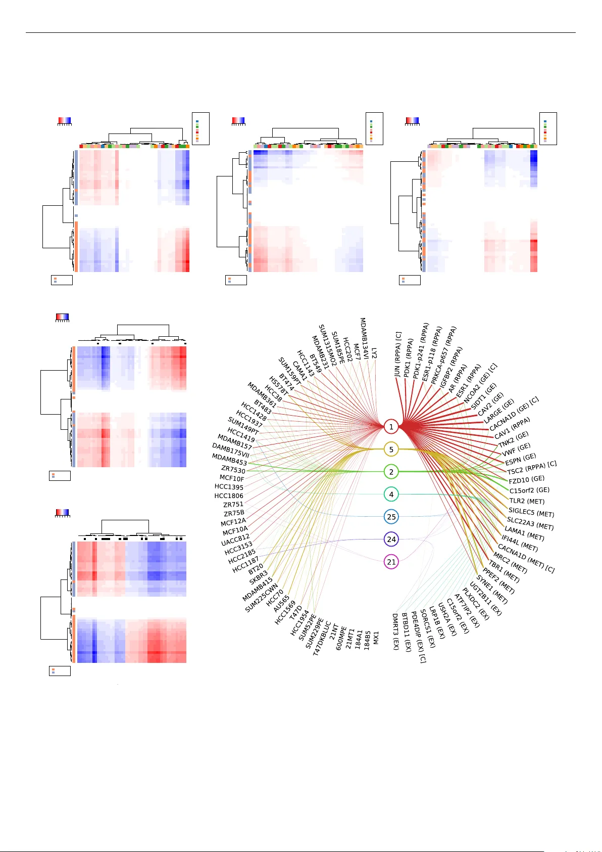
Sparse group factor analysis for biclustering of multiple data sources K erstin Bunte 1 , 2 , Eemeli Leppäaho 1 , Inka Saarinen 1 , and Samuel Kaski 1 1 Helsinki Institute for Information T echnology HIIT , Aalto Uni versity , Finland 2 Presently at School of Computer Science, Uni versity of Birmingham, Edgbaston, UK August 19, 2021 Abstract Motiv ation: Modelling methods that find structure in data are neces- sary with the current large volumes of genomic data, and there ha v e been various efforts to find subsets of genes exhibiting consistent patterns ov er subsets of treatments. These biclustering techniques hav e focused on one data source, often gene expression data. W e present a Bayesian approach for joint biclustering of multiple data sources, extending a recent method Group Factor Analysis (GF A) to hav e a biclustering interpretation with additional sparsity assump- tions. The resulting method enables data-driv en detection of linear structure present in parts of the data sources. Results: Our sim- ulation studies sho w that the proposed method reliably infers bi- clusters from heterogeneous data sources. W e tested the method on data from the NCI-DREAM drug sensitivity prediction challenge, resulting in an excellent prediction accuracy . Moreover , the pre- dictions are based on sev eral biclusters which provide insight into the data sources, in this case on gene e xpression, DNA methylation, protein abundance, exome sequence, functional connecti vity finger- prints and drug sensitivity . A vailability: http://research. cs.aalto.fi/pml/software/GFAsparse/ 1 Intr oduction Numerous clustering approaches have advanced to extract knowl- edge from sets of e.g. gene expression experiments, when condi- tions of the samples are either not known or researchers are inter- ested in dependencies within or across experiments. Conditions or treatments can affect the expression le vels of certain genes only , and similarly , many genes are likely to be co-regulated under certain conditions only . For this purpose, biclustering techniques have been dev eloped (Cheng and Church, 2000; Hartigan, 1972; Lazzeroni et al. , 2002; Morgan and Sonquist, 1963). Biclustering is tradition- ally defined as simultaneously clustering both ro ws and columns in a data matrix. Depending on the metric and the data, dif ferent ap- proaches hav e emerged, aiming to cluster genes based on their ex- pression le v els being the same, differing by a constant, or being lin- early dependent, with respect to dif ferent conditions (Madeira and Oliv eira, 2004). Hochreiter et al. (2010) introduced a generative ap- proach called Factor Analysis for Bicluster Acquisition (F ABIA), accounting for linear dependencies between gene expression and conditions. The biclusters are factors of the measurement matrix, and hence can be overlapping in both genes and conditions, whereas many approaches are limited to distinct clusters. Each bicluster can also include oppositely regulated genes (up- and do wn-regulated) across conditions. Similar approaches have been proposed by Car- valho et al. (2008) and Gao et al. (2014), with the latter one addi- tionally focusing on the inference of gene co-expression networks. F ABIA has also been extended to better suit genotype data (Hochre- iter, 2013). W altman et al. (2010) proposed an algorithm for simultaneous bi- clustering of heterogeneous multiple species data collections. They in vestigate the identification of conserved co-regulated gene groups (modules) by comparing genome-wide datasets for closely related organisms and the evolution of gene regulatory networks. Most genes are unlikely to be co-regulated under ev ery possible condi- tion, and exclusi ve gene clusters cannot capture the complexity of transcriptional regulatory networks. Their proposed approach aims to identify meaningful condition-dependent conserved modules, in- tegrating data across the same genes present in multiple species. Inferring bicluster structure jointly from multiple data sources is potentially more accurate than analysis of a single set, and the dis- cov ered relationships between the sources may offer new insights. In this paper , we extend a recent generativ e Bayesian modelling approach, group factor analysis (GF A) (V irtanen et al. , 2012; Su- vitaiv al et al. , 2014; Klami et al. , 2015). GF A was developed for exploratory analysis of multiple data sources (views), resulting in an interpretable group-sparse factorization of the data collection. When the factors are additionally variable-wise sparse, as a result of introducing suitable priors, they are interpretable as biclusters of multiple co-occurring data sources that need not share the same features (genes; as opposed to W altman et al. (2010)). As a fac- tor model GF A further shares the fav ourable properties of F ABIA. W e demonstrate its use in a multi-view drug sensitivity prediction task that the pre vious bicluster methods could not handle naturally: the approach shows superior prediction performance, and is able to infer meaningful structure present in subsets of the data. 2 Methods 2.1 F actor analysis Factor Analysis for Bicluster Acquisition (Hochreiter et al. , 2010) assumes preprocessed and filtered gene expression data Y ∈ I R N × D . Every row represents a sample and e very column a gene. Therefore the value y i,j corresponds to the expression lev el of the j th gene in the i th sample. A bicluster is defined as a set of rows that are similar for a set of columns, and vice versa. The model for K biclusters is Y = K X k =1 x : ,k w > : ,k +  , (1) where each factor k is defined by an outer product of the k th columns of the factor matrix X ∈ I R N × K and the loading ma- trix W ∈ I R D × K , and  ∈ I R N × D is normally distributed noise:  n,d ∼ N (0 , σ 2 d ) . The factors are the biclusters, with | w d,k | indicat- 1 Sparse group factor analysis for biclustering Page 2 ing the (soft) membership of gene d in bicluster k , and | x n,k | like- wise for sample n . Both the W and X are given sparse priors, more specifically component-wise independent Laplace distributions: p ( W ) =  1 √ 2  DK K Y k =1 D Y d =1 e − √ 2 | w d,k | (2) p ( X ) =  1 √ 2  N K K Y k =1 N Y n =1 e − √ 2 | x n,k | . (3) The parameters are inferred with v ariational e xpectation maximiza- tion, see (Hochreiter et al. , 2010) for details. 2.2 Sparse group factor analysis f or biclustering Group factor analysis has been proposed as an extension to factor analysis for finding factors capturing joint variability between data sets instead of individual v ariables (V irtanen et al. , 2012; Suvitai val et al. , 2014; Klami et al. , 2015). It is designed to deal with sev- eral data sources Y (1) ∈ I R N × D 1 , . . . , Y ( M ) ∈ I R N × D M (called views) of dimensionality D m with N co-occurring observations. GF A models the n th sample of the m th data view as y ( m ) n ∼ N  W ( m ) x n , τ − 1 m I D m  , (4) where τ m is the noise precision of view m . The loading matrix W ( m ) is gi ven a sparse prior that allo ws omitting an y component k from affecting drug data view Y ( m ) . This enables a group-sparse factorization, where components may be (i) specific to a single data view , (ii) shared between all the data views or (iii) shared between any subset of the data views. As we are interested in finding biclus- ters, we introduce a prior that is additionally v ariable-wise sparse, that is, across the elements of the matrices W ( m ) and X . This is done similarly to how Khan et al. (2014) produced variable-wise sparsity , but now for both variables and samples to produce biclus- ters. Namely we use the follo wing spike and slab priors 1 : x n,k ∼ h ( x ) n,k N  0 ,  α ( x ) k  − 1  +  1 − h ( x ) n,k  δ 0 (5) w ( m ) d,k ∼ h ( m ) d,k N  0 ,  α ( m ) k  − 1  +  1 − h ( m ) d,k  δ 0 (6) h (:) n,k ∼ Bernoulli ( π (:) k ) π (:) k ∼ Beta ( a π ,b π ) α (:) k ∼ Gamma ( a α ,b α ) (7) where the binary h ( m ) d,k determines whether the component (biclus- ter) k is acti ve in the d th feature of Y ( m ) (for all non-zero n in h ( x ) n,k ), α ( m ) k determines the scale of the component k in vie w m and π ( m ) k the probability of h ( m ) d,k = 1 . The prior is analogous for samples (i.e. the rows of the data matrices) through h ( x ) n,k .Effecti vely , the spike and slab prior will set weights that affect the data (likelihood) only little to 0, which allows direct biclustering interpretations without a need for arbitrary thresholding afterwards. The model is completed with a gamma prior for the noise precision parameters τ m and un- informativ e hyperpriors ( [ a π , b π , a α , b α , a τ , b τ ] = 1 ). In this formulation, the data source information (feature group- ing) is used in three ways: (i) the noise precision ( τ m ) is the same for all the features in a view , (ii) the binary vector h ( m ) : ,k has a 1 Suvitaiv al et al. (2014) included sparsity for samples and mentioned the con- nection to biclustering, but the interpretation was not e xplored further N 1 N 2 D 1 D 2 D 3 Y (1 , 1) Y (1 , 2) Y (2 , 1) Y (3 , 1) Y (1 , 1) Y (1 , 2) Y (2 , 1) Y (3 , 1) Fig. 1: Left : 4 non-overlapping biclusters (coloured blocks) used in the multi-view data (gray area). Right: The biclusters inferred by GF A. common probability ( π ( m ) k ) of being activ e and (iii) the scale of a component ( α ( m ) k ) is shared within a view . W ith an uninforma- tiv e Gamma prior, often called Automatic Rele vance Determination prior , this third property implements the group sparsity . The second property implies that a specific feature d (in view m ) is more lik ely to be activ e in a bicluster , if many of the features in view m belong to the said bicluster , and vice v ersa. This allows explaining variance that is not present in all the data sources, but dense in some of them, more robustly . Giv en data with significant (source specific) struc- tured variation respective components can help to detect biclusters more accurately . The formulation above assumes that all the data views hav e co-occurring samples. W e also extend GF A for joint mod- elling of data sets that are paired in two modes (see Fig. 1), i.e. { Y (1 , 1) , . . . , Y ( M 1 , 1) , Y (1 , 2) , . . . Y ( M 2 , 2) } , where Y ( m, 2) ∈ I R D 1 ,N 2 is paired with the features of Y (1 , 1) . Both the modes will hav e a set of components identical to the ones presented abo ve with one e xception, and hence we will not repeat the details of the priors here. The exception is that the vie w paired in both the modes is generated from the components of both the modes, as y (1 , 1) i,j ∼ N  w (1 , 1) j x (1) i + w (1 , 2) i x (2) j , τ − 1 1 , 1  . (8) As the priors remain conjugate, the model can be inferred using Gibbs sampling, resulting in linear complexity in both N and D , but cubic w .r .t. the number of components K . The parameters shown in this paper , and us ed in predicti ve tasks, will be the posterior means. In the following sections we will test F ABIA and GF A in several simulation studies and a drug sensitivity analysis, incorporating ge- netic data av ailable from the DREAM project. 3 Simulation study W e show an illustrativ e example of bicluster inference, generating a collection of data sets, { Y (1 , 1) , Y (2 , 1) , Y (3 , 1) , Y (1 , 2) } , with 200 samples and dimensions (100 , 50 , 60) for Y (: , 1) , and 100 samples and dimension (70) for Y (1 , 2) . The data collection was generated with four biclusters and additional noise with variance 1. The non- zero parts of x and w for the biclusters were drawn from N (0 , 1) , but truncated between absolute values 1 and 2 for illustrativ e pur- poses. The data structure is shown in Fig. 1 (left); for clarity the biclusters are non-ov erlapping blocks. W e inferred the component structure of these data using GF A; the posterior mean of the biclus- ters is visualized in Fig. 1 (right). GF A can clearly infer this kind of component structure very accurately . GF A has been designed for joint modelling of multiple data sets. Howe ver , when the data consist of one set only , F ABIA and GF A Sparse group factor analysis for biclustering Page 3 are essentially the same model; in the current implementations there is the technical difference that F ABIA has a continuous valued spar- sity prior for X and W , whereas GF A implements a discrete choice with the spike-and-slap. W e first inv estigate the effect of this techni- cal difference by comparing GF A with F ABIA on single-view data (F ABIA1), and then inv estigate how much multi-view data helps, by comparing GF A against F ABIA for which data are concatenated into a single matrix (F ABIA2). For the simulation studies, we construct data from the generativ e model Eq. (4), with matrices X and W generated such that each element is either zero or sampled randomly from the normal distri- bution N (0 , 1) to build the bicluster(s). The resulting data matrices Y are given to the methods, which then return the bicluster esti- mates x 0 : ,k w 0> : ,k . They are compared to the true biclusters to analyse the models’ performance. F ABIA is run with the correct number of biclusters K , and the results are reported for a range of thresholds. GF A learns the cluster number by dri ving unnecessary ones to zero, and we used a component number 5 abov e the correct K . The final biclustering is based on 101 posterior samples (2000 burn-in sam- ples, 20 thinning): if the majority of ( x : ,k w ( m ) > : ,k ) ij are non-zero in the posterior samples, then Y ( m ) ij is assigned to the k th biclus- ter , otherwise not. All the simulation studies are repeated 10 times and we report the av erage F 1 score for detecting the true bicluster structure: F 1 = 2 T P 2 T P + F N + F P (9) where T P , F N and F P denote the number true positives , false ne gatives and false positives , respecti vely , summed ov er all the el- ements of the data matrix. T o be able to ev aluate the effects of different sparsity priors and inference techniques, we also compare to F A with similar priors as GF A, using the full concatenated data, and inferred with Gibbs sampling. This is done be changing Eq. (5) to Eq. (7) to allow only single α (1) k and π (1) k across the data features, and by giving each feature independent noise precision τ d . By default we use M = 5 data views, N = 50 samples, D m = 100 features per data view and one bicluster acti ve in 70% of the samples and the features. Bicluster and noise variance in the view of interest are set to 1. T o make the data views hetero- geneous, the other 4 data vie ws are giv en bicluster and noise vari- ances of ((0 . 2 , 0 . 2) , (5 , 5) , (0 . 2 , 5) , (5 , 0 . 2)) . W e report the mean performance of the methods in Fig. 2, in six different experimental settings: (a) All data vie ws are set to be homogeneous having v ariance of 1 in the bicluster and the noise residual, and the number of data views is varied. Due to the homogeneity of the data views, GF A has no advantage o ver F A. F A outperforms F ABIA on high-dimensional large number of vie ws. (b) Similar to (a), but with heterogeneous data with respect to the bicluster and noise residual strength. The multi-view approach of GF A is superior , while F A and F ABIA have similar performance. (c) Similar to (b), but with sparse biclusters w .r .t. the samples and group sparse w .r .t. the features (present in all but ev ery 3rd vie w). This matches GF A ’ s assumptions leading to superior results. (d) Additional view-specific noise components (0 to 6) were added on top of the bicluster signal (as x noise w > noise , each vector element sampled from N (0 , 1) ). The GF A-type of priors and inference are clearly more robust against the structured noise. (e) W e ev aluated the accuracy of detecting 1 to 7 partly overlapping biclusters. GF A outperforms F A, whereas F ABIA does not seem ● ● ● ● ●●● ● ● ● ● ● ● ● ● ● ● ● ● ● ● ● ● ● ● ● 0.70 0.75 0.80 0.85 1 10 100 Number of views M F1 (a) Homogeneous data views ● ● ● ● ●●● ● ● ● ● ● ● ● ● ● ● ● ● ● ● ● ● ● ● ● 0.70 0.75 0.80 0.85 1 10 100 Number of views M F1 (b) Heterogeneous data views ● ● ● ● ●●● ● ● ● ● ● ● ● ● ● ● ● ● ● ● ● ● ● ● ● 0.70 0.74 0.78 0.82 1 10 100 Number of views M F1 (c) Group−sparse biclusters ● ● ● ● ● ● ● ● ● ● ● ● ● ● 0.6 0.7 0.8 0 1 2 3 4 5 6 Number of structured noise components F1 (d) Structured source−specific noise ● ● ● ● ● ● ● ● ● ● ● ● ● ● 0.65 0.70 0.75 0.80 0.85 1 2 3 4 5 6 7 Number of biclusters F1 (e) Multiple par tly o verlapping biclusters ● ● ● ● ● ● ● ● ● ● ● ● ● ● ● ● ● ● 0.68 0.72 0.76 0.80 0.84 0.1 10.0 Bicluster strength in supporting views F1 (f) V ar ying bicluster strength Model:     GF A F A F ABIA1 F ABIA2 Threshold ● auto 0.01 0.05 0.1 Fig. 2: Simulated experiments comparing the abilities of GF A, F A and F ABIA to detect data-generating biclustering. (a) and (b) report the F 1 scores o ver a varying number of data vie ws ( M ) present, for homogeneous and heterogeneous data collections, respecti vely . The biclusters are further assumed group-sparse in (c). In (d) the problem is made more challenging by adding structured noise on top of the signal, whereas the number of biclusters is varied in (e). In (f), the strength of the bicluster is v aried in the supporting vie ws. F ABIA1 uses only the data matrix of interest, whereas F ABIA2 and F A have side information concatenated with it; both F ABIAs are reported for thresholds (0 . 01 , 0 . 05 , 0 . 10) determining the biclusters. very robust when the number of biclusters increases; using the additional data can ev en decrease its performance. (f) The strength of the biclusters is varied for the additional views (precision α ranging from 10 − 2 to 10 2 ). GF A is more accurate when the additional views ha ve strong biclusters, and has a simi- lar performance with F ABIA when weaker . F A suffers compared to F ABIA when the additional views get less rele vant. Across all the studies discussed above, GF A was able to detect the correct number of biclusters (and additional noise components) exactly in 90.4 % of the runs, and overestimated it by 1, 2 or 3 in 9% , 0 . 4% and 0 . 1% of the runs, respecti vely . The extra components were modelling artificial structure detected in the residual noise and did not resemble the bicluster structure. T o confirm that they did not giv e an advantage in the comparison, we also ran F ABIA with 5 ex- tra components, resulting in consistently worse performance com- pared to the reported runs, where F ABIA was given the true com- ponent amount. The standard deviations of the mean F 1 scores, av eraged over the 10 independent repetitions, ranged from 0.003 to 0.01. Inferring a single model took on average 22s, 45s, 0.04s, and 0.5s for GF A, F A, F ABIA1 and F ABIA2, respectively , demonstrat- ing the efficienc y of the EM-algorithm in F ABIA. Our F A implementation is generally , but not consistently , more Sparse group factor analysis for biclustering Page 4 robust than F ABIA in bicluster detection with additional data sources. The adv antages of the multi-vie w setup of GF A (vs con- catenation in F A and F ABIA2) are most significant when (i) there are plenty of heterogeneous data views, (ii) the biclusters are group- sparse, or (iii) the data views are highly heterogeneous. These con- ditions are realistic in real-life applications. 4 Drug response study The NCI-DREAM drug sensitivity prediction challenge (Costello et al. , 2014) provided publicly a vailable data consisting of gene e x- pression (GE), RN A, DNA methylation (MET), copy number vari- ation (CNV), protein abundance (RPP A) and exome sequence (EX) measurements for 53 human breast cancer cell lines. In the chal- lenge, expression data were based on Affymetrix Genome-W ide Human SNP6.0 Array and Affymetrix GeneChip Human Gene 1.0 ST microarrays. RNA sequencing libraries were prepared using the T ruSeq RNA Sample Preparation Kit and whole transcriptome shot- gun sequencing was performed. The Mutation status was obtained from exome-capture sequencing and GenomeStudio Methylation Module v1.0 was used to express the methylation for each genome- wide detected CpG locus resulting in values between 0 (completely unmethylated) to 1 (completely methylated) proportional to the de- gree of methylation at any particular locus. More details on the preparation of the genomic data for the challenge are provided by Costello et al. (2014). Each cell line was exposed to 31 therapeutic compounds and the dose-response v alues of gro wth inhibition were collected. The drug response data was revealed only for 35 of the cell lines, and the challenge was to predict the response of the re- maining 18 cell lines, ranking them from the most sensitiv e to the most resistant. As the drug response prediction problem is extremely challeng- ing, we performed the follo wing steps, learning from Costello et al. (2014), to increase the signal-to-noise ratio: W e reduced the dimen- sionality to the 500 genes with the highest a verage variance over the data views, including the ov erlapping set of 14 genes appearing in the RPP A data set. Furthermore, the most predictive data sources for further analysis were chosen by 7-fold cross validation on the 35 training samples with known drug response v alues. T o compare the sources the root mean squared error (RMSE), as well as Pearson and Spearman correlations of the predicted drug responses, were computed av eraged over 10 repetitions of the experiments, each with different random splits. W e inferred the GF A model for this multi-view data by ignoring the missing drug response data in the likelihood, after which the missing values can be predicted from XW ( m ) , where X for the missing cell lines is inferred based on the other data sources only . The performance of GF A trained with different combinations of data vie ws is shown in T able 1. The most promising views finally chosen for the bicluster analy- sis were gene expression, methylation, exome sequence and RPP A measurements, leaving out the copy number variation and RNA. Finally , we ran GF A for the full data (handling the test drug re- sponses as missing v alues) and reconstructed the missing data av- eraged ov er the posterior samples of 50 sampling chains. W e gav e the model a mildly informativ e prior assuming signal-to-noise ratio of 0.5. All the sampler chains were initialized with K = 60 , al- lowing data-driven inference of model complexity (resulting in 48 to 56 components). A total of 100 sampled parameters were stored for each chain (ev ery 20th sample stored after 10000 burn-in itera- tions), resulting in an a verage runtime of 84 minutes per chain. The performance was quantified using the same score as in the chal- T able 1: A veraged 7-fold cross validation results for GF A on the training set of the DREAM7 drug sensitivity prediction challenge to identify the views sho wing best prediction performance for further analysis. V iews used RMSE Pearson Spearman All 1.9 0.031 0.079 GE, MET , CNV , RN A, RPP A 2.3 0.016 0.088 GE, CNV , RN A, RPP A, EX 2.0 0.031 0.078 GE, MET , CNV , RPP A, EX 1.5 0.040 0.085 GE, MET , CNV , RN A, EX 1.8 0.012 0.078 MET , CNV , RN A, RPP A, EX 1.6 0.018 0.058 GE, MET , RNA, RPP A, EX 1.9 0.040 0.089 GE, MET , CNV , RPP A 1.8 0.028 0.071 GE, CNV , RPP A, EX 1.8 0.018 0.074 GE, MET , CNV , EX 1.5 0.024 0.090 MET , CNV , RPP A, EX 2.1 0.020 0.061 GE, MET , RPP A, EX 1.4 0.046 0.087 GE, MET , RPP A 1.9 0.024 0.072 GE, RPP A, EX 1.6 0.016 0.059 GE, MET , EX 1.5 0.042 0.084 MET , RPP A, EX 1.8 0.011 0.075 lenge, that is, the weighted averaged probabilistic concordance in- dex. W e achieved a score of 0.592, which would have been placed the first in the challenge (winner model reaching 0.583), indicat- ing excellent prediction performance of GF A on this data, possibly stemming from the biclustering nature of the model. Furthermore, we ran GF A utilizing data sources paired in two modes in a similar way with additional functional connectivity fingerprints describing the drugs (FCFP; calculated with PaDEL-Descriptor , Y ap (2011)), allowing joint modelling of biological and chemical effects in the measured data. The additional chemical view resulted in a slight in- crease in the target score, to 0.599.The structure of the latter model is interpreted in the following sections, motiv ated by the excellent predictiv e performance. 4.1 Robust components For interpretation purposes we next sought representative point so- lutions to describe the posterior distributions. Due to the extremely challenging nature of the problem the total variance explained by individual components is small. T o minimize the risk of analysing patterns occurred by chance, we searched for components that oc- cur consistently across the different sampling chains, making the assumption (which was checked manually) that component indices are reasonably stable within a chain, but can naturally be arbitrar- ily permuted between chains. T o find the matches between chains we av eraged the components o ver the posterior samples within their chain, and compared using cosine similarity . If the similarity of the best match exceeded the threshold 0.80, we considered the com- ponents to be the same. Furthermore, we chose to further study components found in at least half of all chains, deemed robust in this procedure. Out of the a verage 52.6 components inferred by the sampling chains, 25 were on average chosen to the set of robust components. Ideally we would infer the model parameters with a single well-mixing sampling chain, but as the posterior is multi- modal (and we do not want to constrain it artificially) the inference problem is extremely challenging, and we resort to the described computational simplification. W e observed that some of the components are very sparse, only containing one or two cell lines and hence most probably explaining outliers in the data. Therefore, we will focus the interpretations on the more dense biclusters only; 3 out of the total 27 biclusters found Sparse group factor analysis for biclustering Page 5 predicted 1.26%, 0.06% and 0.11% of the total variance in the test data (2.89%, 0.3% and 0.98% in the set of acti ve drugs). There was 1 additional bicluster shared with the drug descriptors, but it had no significant effect to the test data. W ith the drug sensitivity prediction of these four components only , we received a target score of 0.591. 4.2 Interpr etations of the biclusters For interpretation purposes, we collected the descriptions of the drugs and cell lines used in the challenge (Costello et al. , 2014). Some groups of drugs can be identified, which we will abbrevi- ate as: autophagy (au), cell cycle (cc), metabolism (me), regulation (re) and signalling growth (gr) drugs, as well as nuclear factor (nf), protease (pr) and receptor tyrosine kinase (rtk) inhibitors. Further- more, most of the cell lines represent a subtype of cancer which can be categorized as basal or luminal. The bicluster structure of the acti vity patterns for the first compo- nent in the drug sensitivity (DS) view , consisting of measurements of sensitivity of cell lines to drugs, is depicted in Fig. 3a. Com- ponent one distinguishes basal and luminal cell types, without that information being used in the training. The response for all 5 cell cycle and all 4 metabolism drugs is positive or above average for most of the basal cell lines, whereas luminal cells show negativ e ac- tiv ation. Luminal cells respond strongly to regulation drugs, where the response of basal cells is neg ativ e. Component 2 shows high activity patterns for proteasome and cell cycle drugs as depicted in Fig. 3b. The other components hav e relati vely small biclusters with only a few activ e cells and drugs. Component 3, for example, shows cells that are (un)responsiv e to rtk inhibitors and otherwise mixed groups of cells and drugs (see Fig. 3c). The remaining robust com- ponent, in the second mode, was associated with most of the drugs and drug descriptors, and weakly with approximately half of the cell lines (strongly with T47DKBLUC). Due to the large number of genes in the other vie ws, we show summaries of enrichment of kno wn cancer genes in the compo- nents. W e performed hypergeometric tests comparing a varying number of the most active genes (i.e. genes with the highest mean absolute values in W corresponding to RPP A and GE views) and random sets of equal size, for the occurrence of known cancer genes (extracted from Stephens et al. (2012)) in the most predictive com- ponents and all vie ws. Low p -values indicate that the approach is able to detect a significant amount of known (breast) cancer genes in the top active genes of the components when compared to ran- dom subsets of genes in the vie ws. Fig. 4 sho ws the results of the hypergeometric test for two robust components. For component 1 (Fig. 4a) we observe highly significant cancer activity already in the 10 most active genes in ev ery view , except in the RPP A data. In the Exome sequence data we observe significant cancer gene acti v- ity independently of the size of the subset. For component 2 (Fig. 4b) we observe less significant activity of cancer genes in the gene expression and e xome data than in component 1. Howe ver , we find high cancer gene acti vity in the methylation view and v ery high ac- tivity of breast cancer genes in e xome sequencing data. Besides the statistical tests we report the results on the level of individual genes. W e condensed the analysis sho wing the 5 0 most activ e genes (in terms of their absolute values) in component 1 in the gene expression (Fig. 3d) and the RPP A view in Fig. 3e. Com- ponent 1 contains proportional and anti-proportional co-regulated genes as indicated by the intensity of the biclusters depicted. The genes which are known as cancer or breast cancer genes are mark ed 0.0003 0.0010 0.0030 0.0100 0.0500 0.3000 1.0000 10 20 30 40 50 60 70 80 90 100 150 200 number of genes hypergeometric p−v alue type ● ● BC C view GE MET RPP A EX (a) Cancer gene activity in component 1 0.003 0.010 0.050 0.300 1.000 10 20 30 40 50 60 70 80 90 100 150 200 number of genes hypergeometric p−v alue type ● ● BC C view GE MET RPP A EX (b) Cancer gene activity in component 2 Fig. 4: Hypergeometric test of the activity of kno wn breast cancer (BC) and all cancer (C) genes in the two most predicti ve components and all vie ws. Low P-v alues indicate a high number of cancer genes in the top n activ e genes in comparison with randomly picked sets. See the text for details. by a black and gray squares, respecti vely . Fig. 3f summarizes the mean participation in biclusters of the cells in seven different components on the top 10 active genes in each of the views. The left side contains the list of all cells sorted by their mean absolute values in the seven most active components, which are depicted in the middle row . The right side contains the list of top genes clustered by their mean activity in these components, accompanied by a shortcut for the view they were taken from and [C] in case they are kno wn as cancer gene in the literature. Component one (coloured red) contains the biggest biclusters with comparably high mean absolute values depicted by thicker connecting lines in lots of cells and genes throughout the different views except the exome sequence data. Even only selecting 10 most acti ve genes from each view delivers at least one known cancer gene. Although compo- nents overlap the y also depict relationships of different cells in dif- ferent views. Furthermore, we performed a Gene Ontology (GO) enrichment analysis on the most activ e gene sets in the components and gene related vie ws. In GO the genes or gene products are hierarchically classified and grouped into three categories: molecular function (mf) describing the molecular acti vity of a gene, biological pr ocess (bp) denoting the larger cellular role and cellular component (cc) depicting where the function is executed in the cell. The enrich- ment analysis was performed directly in the GO website ( http: //geneontology.org/ ), which connects the P ANTHER (Mi et al. , 2013) classification system with GO annotations. From each of the gene-related views GE, MET , RPP A and EX we selected a list of the 50 most activ e genes from the dense robust components. For each of such gene sets we calculated the enrichment for all cat- egories. The result table contains a list of shared GO terms for each gene set together with information about the background and sample frequenc y , fold enrichment and the p-v alue determined by a binomial statistic. A p-v alue close to zero indicates the significance of the GO term associated with the provided group of genes. More than one thousand shared GO terms are returned for the most active gene sets. W e condensed the results showing only the most repeating and most significant ones by using a threshold for the p-value and sho wing only GO terms below 10 − 6 , which appear Sparse group factor analysis for biclustering Page 6 (a) DS: Robust Component 1 subtypes drugtypes IKK16 MG−132 OlomoucineII Disulfiram MG−132b Baicalein Chloroquine MG−115 PD184352 Doxorubicin Methylglyoxol Mebendazole Bromopyruvate TCS−PIM−11 Nilontinib Cetuximab 4−HC+Dox unknown2 unknown3 unknown1 4−HC B581 Imatinib PS−1145 GW5074 T rastuzumab Nelfinavir QNZ FR180304 Everolimus Valproate HCC38 BT549 MDAMB157 SUM159PT HS578T SUM1315MO2 HCC1143 MDAMB231 MCF12A MCF10A HCC3153 HCC1937 SUM149PT MCF10F HCC1395 HCC1806 BT20 HCC1954 HCC70 HCC1569 HCC1187 SUM229PE 21NT 21MT1 600MPE MX1 184B5 T47DKBLUC 184A1 AU565 SKBR3 SUM52PE MDAMB415 HCC2185 ZR75B SUM225CWN CAMA1 MDAMB361 BT474 BT483 HCC1419 SUM185PE MDAMB175VII T47D HCC1428 MCF7 ZR7530 L Y2 HCC202 MDAMB134VI MDAMB453 ZR751 UACC812 Activity in component 1 −0.6 0.2 V alue Color Key drugtypes au cc gr me nf pr re rtk basal luminal (b) DS: Robust Component 2 subtypes drugtypes Mebendazole Disulfiram T rastuzumab Chloroquine PS−1145 Doxorubicin 4−HC IKK16 PD184352 Imatinib 4−HC+Dox Valproate MG−132b TCS−PIM−11 unknown1 unknown3 Cetuximab Bromopyruvate Nilontinib unknown2 MG−115 QNZ Methylglyoxol Everolimus FR180304 OlomoucineII GW5074 Baicalein Nelfinavir B581 MG−132 BT483 MDAMB415 HCC38 HCC1937 HCC1419 HCC1428 MDAMB361 CAMA1 MDAMB157 HCC1143 BT20 BT474 MCF10F BT549 HCC1954 HCC1395 HCC1187 HS578T HCC3153 MDAMB134VI ZR75B MDAMB231 SUM1315MO2 UACC812 SUM185PE SUM229PE 21NT MX1 T47DKBLUC 600MPE HCC1569 184A1 184B5 21MT1 HCC202 AU565 ZR751 MCF12A HCC2185 MCF10A HCC1806 SUM225CWN SUM159PT HCC70 T47D SUM52PE MCF7 L Y2 MDAMB175VII SKBR3 SUM149PT ZR7530 MDAMB453 Activity in component 2 −0.3 0.2 V alue Color Key drugtypes au cc gr me nf pr re rtk basal luminal (c) DS: Robust Component 5 subtypes drugtypes Imatinib Nelfinavir MG−132b OlomoucineII PS−1145 Everolimus MG−115 Cetuximab Nilontinib PD184352 Disulfiram T rastuzumab unknown2 unknown3 GW5074 Bromopyruvate 4−HC+Dox Methylglyoxol 4−HC IKK16 Baicalein Doxorubicin Mebendazole Chloroquine unknown1 QNZ Valproate FR180304 B581 TCS−PIM−11 MG−132 L Y2 MDAMB134VI MDAMB175VII MCF7 SUM52PE HCC1569 BT474 BT549 MDAMB231 HCC1143 HCC1954 CAMA1 MDAMB453 BT20 HCC1937 ZR7530 SUM185PE HCC3153 MDAMB361 UACC812 MCF12A ZR751 BT483 HCC1806 ZR75B HCC1395 21MT1 184A1 184B5 MCF10F 21NT 600MPE MX1 SUM229PE T47DKBLUC HCC1419 MCF10A HCC38 HCC2185 HCC1187 MDAMB157 HCC202 HCC1428 SUM149PT SUM1315MO2 T47D SUM159PT HCC70 MDAMB415 AU565 HS578T SUM225CWN SKBR3 Activity in component 5 −0.15 0.1 V alue Color Key drugtypes au cc gr me nf pr re rtk basal luminal (d) T op 50 Genes in GE view subtypes known cancer known breast cancer ST6GALNAC3 TRPC4 TMEFF2 SIRPB1 NUMBL PDE3A SYNE1 RGS4 TLR2 FLI1 PDE8A CAV2 SACS CFH BNC2 LP A MRGPRX4 CBS ME3 HOOK3 SLC22A3 MGST1 TG GPC6 TJP2 IFI44L MAGI2 BTBD11 L YST SLC24A2 TTLL3 NTSR1 MYOM2 C18orf34 FGFR3 C20orf85 C10orf129 UGT2B11 NELL2 ARHGEF5 ZNF85 PTPRT C1orf51 UBC TNK2 PPP2R2C PGR SHANK2 NEBL NCOA2 UACC812 ZR751 MDAMB134VI MDAMB453 HCC202 L Y2 HCC1428 MCF7 ZR7530 T47D MDAMB175VII HCC1419 SUM185PE BT483 BT474 MDAMB361 CAMA1 ZR75B SUM225CWN HCC2185 MDAMB415 SUM52PE AU565 SKBR3 HCC1187 184A1 T47DKBLUC 21MT1 184B5 MX1 SUM229PE 21NT 600MPE HCC1569 HCC70 HCC1954 BT20 HCC1806 HCC1395 MCF10F HCC1937 HCC3153 SUM149PT MCF12A MCF10A MDAMB231 HCC1143 SUM1315MO2 HS578T SUM159PT MDAMB157 HCC38 BT549 GE: top 50 Genes in component 1 −1.5 1 V alue Color Key basal luminal (e) T op 50 Genes in RPP A view subtypes known cancer known breast cancer PRKCA−p657 PRKCA MAPK14−p ST A T3 MAPK1,MAPK3 CCNB1 ST A T3−p705 CAV1 JUN COL6A1 EN1 EGFR MAP2K1 CCNE1 KDR CDKN1A SRC−p527 YBX1 AKT1−p308,AKT2 −p308,AKT3−p308 CTNNB1 EGFR−p1068 TP53 PIK3CA PRKAA1−p EIF4EBP1 EIF4EBP1−p37 MAPK14 CASP7 PECAM1 CCND1 RPS6KB1−p389 CDH1 PDK1−p241 ESR1−p118 PDK1 ESR1 AR IGFBP2 TSC2 GA T A3 AKT1,AKT2,AKT3 RPS6KB1 KIAA1324 GSK3A,GSKB RAB25 ERBB2 PGR PTEN COMT ERBB2−p1248 BT549 HCC38 MDAMB157 SUM159PT HS578T SUM1315MO2 HCC1143 MDAMB231 MCF12A MCF10A HCC3153 HCC1937 SUM149PT MCF10F HCC1395 BT20 HCC1806 HCC1954 HCC70 HCC1569 HCC1187 21NT 600MPE SUM229PE MX1 184B5 21MT1 184A1 T47DKBLUC AU565 SKBR3 SUM52PE MDAMB415 HCC2185 ZR75B SUM225CWN CAMA1 MDAMB361 BT474 BT483 SUM185PE HCC1419 MDAMB175VII T47D HCC1428 ZR7530 MCF7 L Y2 HCC202 MDAMB134VI MDAMB453 ZR751 UACC812 RP: top 50 Genes in component 1 −1.5 0.5 V alue Color Key basal luminal (f ) Summary 7 robust comp onen ts: Cell lines and top 10 genes in all views Fig. 3: Bicluster acti vity patterns of rob ust components. (a)-(c) sho w the intensity v alues of cells (in rows) and drugs (in columns) in the drug sensiti vity (DS) view of 3 different components. Component one mainly distinguishes basal and luminal cell lines, while (d) and (e) show the corresponding bicluster acti vity pattern of the 50 genes with highest mean absolute v alues in the RPP A and GE vie ws, marking kno wn (breast) cancer genes by a (gray) black square. (f) sho ws bicluster participation of all cells (left) in 7 selected robust components (middle) with respect to their mean absolute intensity values (represented in the thickness of the lines) for the top 10 genes in each of the views (GE, MET , RPP A and EX). Known cancer genes are marked by [C]. Sparse group factor analysis for biclustering Page 7 ● ● ● ● ● ● ● ● ● ● ● ● ● ● ● ● ● ● ● ● ● ● ● ● ● ● ● ● ● ● ● ● ● ● ● ● ● ● ● ● ● ● ● ● ● ● ● ● ● ● ● ● ● ● ● ● ● ● ● ● ● ● ● ● ● ● ● ● ● ● ● ● ● ● ● ● ● ● ● ● ● ● ● ● axon dev elopment axon guidance axonogenesis cell morphogenesis involved in diff erentiation cell morphogenesis involved in neuron diff erentiation epithelium dev elopment extracellular matrix organization extracellular structure organization gland dev elopment neuron projection dev elopment neuron projection guidance neuron projection morphogenesis positive regulation of cell migration positive regulation of cell motility positive regulation of cellular component mov ement positive regulation of locomotion regulation of cell migration regulation of cell motility regulation of cellular component movement adherens junction anchoring junction extracellular matrix plasma membrane region postsynapse proteinaceous extracellular matrix synapse synapse part growth factor binding 3 3.5 4 4.5 >5 fold enrichment term view ● Ex GE Me RP GO ● ● ● bp cc mf Significant GO terms Fig. 5: Enrichment of the most significant GO terms, which occur more than 3 times in all the gene related vie ws and the three dense robust com- ponents. throughout the views and components more than 3 times. Fig. 5 shows the reduced list of significant GO terms with fold enrichment value bigger than 3. This value indicates the magnitude of fold en- richment for the observed set of genes over the expected, thus with values bigger than one the category implying over -representation. For biological process we found most of the repeating significant GO terms in all of the views in nearly all cases. These GO terms are related to cell motility and its regulations. 5 Discussion W e presented sparse group factor analysis as a way of inferring bi- clusters from heterogeneous multi-source data. The method is able to detect predictiv e and interpretable structure present in any subset of the data sources, and sparse within the sources. It proved to be robust in this task, as witnessed by the simulation studies and the outstanding performance in the NCI-DREAM drug sensitivity pre- diction challenge. The biclusters of the joint data identified cancer cell subtypes, grouped drugs by their functional mechanisms, and associated known cancer genes with the drug sensiti vity data, all in a data-driv en fashion. The shown approach is suitable for ex- ploratory analysis of multiple data sources, giving condensed and interpretable information with respect to the data collection. In this paper we focused on formulating a model that implements the novel multi-data-source biclustering, and on ev aluating the ac- curacy of the results. T wo important questions we did not yet fully address are: (i) Could some of the alternative ways of im- plementing sparsity , substituting the spike-and-slabs of this paper , result in computationally more ef ficient and still as accurate so- lutions. (ii) Computational speed. The EM point estimates the single-data-source F ABIA algorithm uses would naturally be faster for multiple data sources as well, but the ability to handle uncer- tainty due to highly noisy and high-dimensional small sample-size data would suffer . V ariational approximations would be attractiv e as they would also help av oid the matchings between the differ - ent sampling chains, but deriving variants of the algorithm would be more difficult and variational approximations are known to pro- duce a biased estimate of the uncertainty of the solutions. For lar ge data parallelised sampling solutions would be particularly attractive ways of speeding up computation. Acknowledgement W e thank the Academy of Finland (Finnish Centre of Excellence in Computational Inference Research COIN) for funding. Refer ences Carvalho, C. M., Chang, J., Lucas, J. E., Nevins, J. R., W ang, Q., and W est, M. (2008). High-dimensional sparse factor modeling: applications in gene expression genomics. Journal of the Ameri- can Statistical Association , 103 (484), 1438–1456. Cheng, Y . and Church, G. M. (2000). Biclustering of expression data. In Proc. of the 8th International Confer ence on Intelligent Systems for Molecular Biology , pages 93–103. AAAI Press. Costello, J. C., Heiser, L. M., et al. (2014). A community effort to assess and improve drug sensitivity prediction algorithms. Natur e Biotechnology , 32 (12), 1202–1212. Gao, C., Zhao, S., McDo well, I. C., Brown, C. D., and Engel- hardt, B. E. (2014). Differential gene co-e xpression networks via Bayesian biclustering models. arXiv preprint . Hartigan, J. A. (1972). Direct clustering of a data matrix. Journal of the American Statistical Association , 67 (337), 123–129. Hochreiter , S. (2013). HapF ABIA: identification of very short seg- ments of identity by descent characterized by rare variants in large sequencing data. Nucleic Acids Res , 41 (e202). Hochreiter , S., Bodenhofer , U., et al. (2010). F ABIA: factor analy- sis for bicluster acquisition. Bioinformatics , 26 (12), 1520–1527. Khan, S. A., V irtanen, S., Kallioniemi, O. P ., W ennerberg, K., Poso, A., and Kaski, S. (2014). Identification of structural features in chemicals associated with cancer drug response: a systematic data-driv en analysis. Bioinformatics , 30 (17), i497–i504. Klami, A., V irtanen, S., Leppäaho, E., and Kaski, S. (2015). Group factor analysis. IEEE T ransactions on Neural Networks and Learning Systems , 26 (9), 2136–2147. Lazzeroni, L., Owen, A., et al. (2002). Plaid models for gene ex- pression data. Statistica Sinica , 12 (1), 61–86. Madeira, S. C. and Oli veira, A. L. (2004). Biclustering algorithms for biological data analysis: A survey . IEEE/ACM T ransactions on Computational Biology and Bioinformatics , 1 (1), 24–45. Mi, H., Muruganujan, A., Casagrande, J. T ., and Thomas, P . D. (2013). Large-scale gene function analysis with the P ANTHER classification system. Nature Pr otocols , 8 (8), 1551–66. Morgan, J. N. and Sonquist, J. A. (1963). Problems in the analysis of survey data, and a proposal. Journal of the American Statisti- cal Association , 58 (302), 415–434. Stephens, P . J., T arpey , P . S., Davies, H., V an Loo, P ., Greenman, C., W edge, D. C., Nik-Zainal, S., Martin, S., V arela, I., Bignell, G. R., et al. (2012). The landscape of cancer genes and muta- tional processes in breast cancer . Nature , 486 (7403), 400–404. Suvitaiv al, T ., Parkkinen, J. A., V irtanen, S., and Kaski, S. (2014). Cross-organism toxicogenomics with group factor analysis. Sys- tems Biomedicine , 2 (4), 71–80. V irtanen, S., Klami, A., Khan, S. A., and Kaski, S. (2012). Bayesian group factor analysis. In N. Lawrence and M. Girolami, editors, Pr oc. of the 15th International Confer ence on Artificial Intelli- gence and Statistics , pages 1269–1277. W altman, P ., Kacmarczyk, T ., Bate, A., Kearns, D., Reiss, D., Eichenberger , P ., and Bonneau, R. (2010). Multi-species inte- grativ e biclustering. Genome Biology , 11 (9), R96. Y ap, C. W . (2011). PaDEL-descriptor: An open source software to calculate molecular descriptors and fingerprints. J ournal of Computational Chemistry , 32 (7), 1466–1474.