Binary Decision Diagrams for Affine Approximation

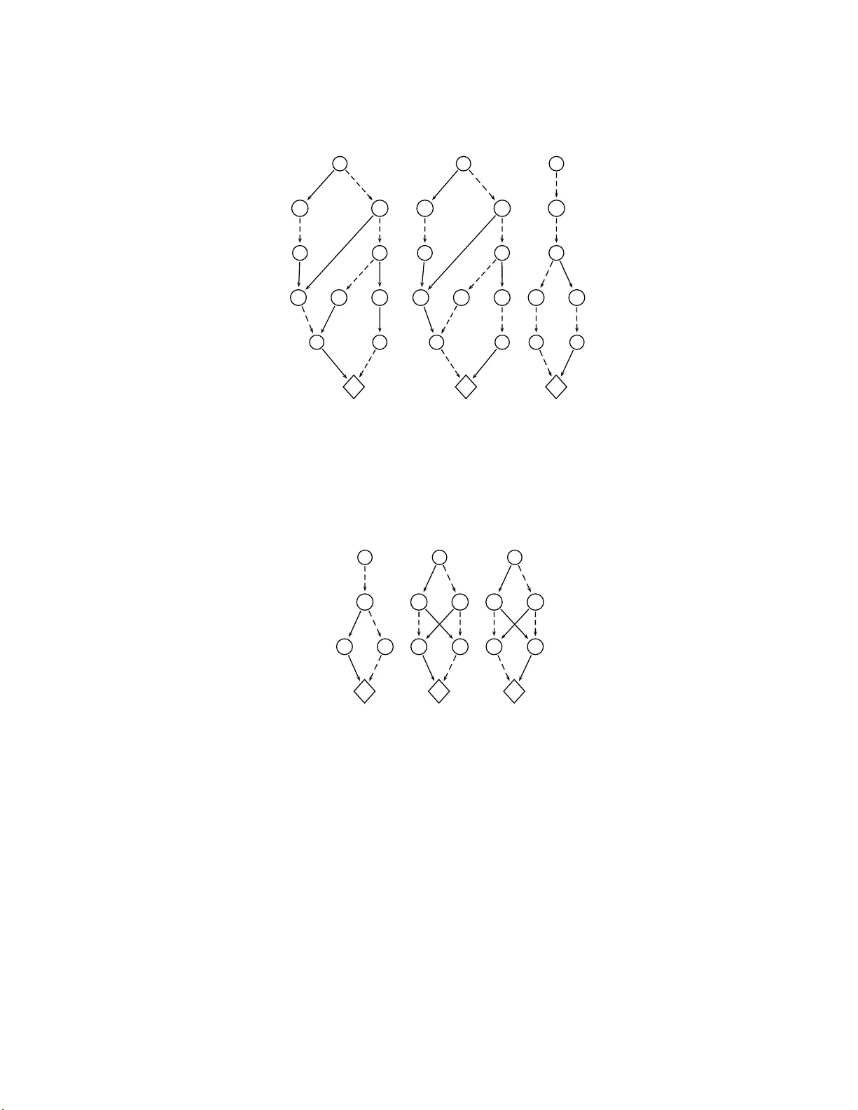
Binary Decision Diagrams for Affine Appro ximation Kevin Henshall, Peter Sc hach te, Harald Sønderga ard and Leigh Whiting Department of C omputer Science and Softw are Engineering The Universi ty of Melbourn e, Vic. 3010, Au stralia Abstract. Selman and Kautz’s work on “knowledge compilatio n” estab- lished ho w approximation ( stren gthening and /or w eak ening) of a propo- sitional knowledge-base can be used to speed up q uery pro cessing, at the exp ense of completeness. In t h is classical approach, querying uses H orn o ver- and under- approximatio ns of a g iven know ledge-base, which is rep- resen ted as a prop ositional form ula in conjunctive normal form (CNF). Along with the class of Horn fun ct ions, one could imagine other Bo olean function classes that might serve the same purp ose, owing to attractive deduction-computational prop erties similar to those of the Horn func- tions. I ndeed, Zan uttini has suggested that the class of affine Bo olean functions could be useful in kn o wledge compilatio n and has presented an affine approximation algorithm. Since CNF i s awkw ard for prese nting affine functions, Zanuttini considers b oth a sets-of-models rep resen tation and the u se of modu lo 2 congruence equations. In this pap er, we pro- p ose an algorithm based on reduced ordered binary decisio n diagrams (ROBDDs). This leads to a representation which is more compact th an the sets of mo dels and, once we hav e established some useful prop erties of affine Bo olean functions, a more efficient a lgorithm. 1 In tro duct ion A r ecurrent theme in artificial in telligence is the efficient use of (prop ositional) knowledge-bases. A promising appr o ach, which was initially prop osed by Selman and Kautz [11], is to query (and perform deductions from) upp er and low er approximations, commonly called envelo p es and c or es resp ectively , of a given knowledge-base. By c ho osing a pproximations that allo w mor e e fficie nt inference , it is often p oss ible to quickly determine that the env elop e of the given knowledge- base entails the query , and therefore so does the full kno wledge-ba se, av oiding the costly inference from the full knowledge-base. When this fails, it may b e po ssible to quickly show that the quer y is not entailed by the core, and therefor e not entailed by the full knowledge-bas e . Only whe n b oth of these fail must the full knowledge-base b e used for inference. It is usually assumed t hat Bo ole an functions a re represented in clausa l form, and that approximations are Horn [11,5], as inference from Horn knowledge- bases is exp onentially more efficient than fro m unrestr ic ted knowledge-base s. How ever, it has been noted that there are other well-understo o d clas s es that hav e co mputational prop erties that include some o f the attractive prop er ties o f the Horn class. Zanuttini [12 ,13] discus ses the use of o ther class es of Boo lean functions for approximation a nd po in ts out that affine a pproximations have certa in adv an- tages o ver Horn approximations, most notably the fact that they do not blo w out in size. This is cer tainly the case when a ffine functions are r epresented in the form of mo dulo-2 congr uence equatio ns. The more general sets-of-mo dels representation is also considered by Z anutt ini. In this paper , we consider an- other general repres e ntation, namely the well-known R e duc e d Ord er e d Binary De cision Diagr ams (ROBDDs) . W e prove some impo r tant pr op erties of affine functions r epresented as ROBDDs, a nd pr esent a new ROBDD algo r ithm for deriving affine env elop es. The ba lance of the pap er pro c e eds a s follows. In Section 2 we r ecapitulate the definition of the Bo o lean affine class , and we establish some o f their imp ortant prop erties. W e also briefly introduce R OBDDs, but ma inly to fix our notatio n, as w e assume that the reader is f amilia r with Boo lean functions and t heir repr e- sentation as decision diagrams. Section 3 recalls the mo del-base d affine en velope algorithm, and develops our own ROBDD-based algo rithm, along wit h a correct- ness pro o f. Sectio n 4 describes our testing m etho dolo gy , in cluding our algorithm for generating random ROBDDs, and pres ent s our results. Section 5 discusses related work and applications , and concludes. 2 Prop ositional Classes, Appro ximation and R OBDDs W e use R OBDDs [1,2] to represent Bo olea n functions. Horiy ama and Ibaraki [6] hav e recommended ROBDDs as suitable for implemen ting knowledge ba ses. Our choice of ROBDDs as a data structure w as not so muc h influenced by that rec - ommendation, as by the c o nv enience of w orking with a canonica l representation for Boolea n functions, and o ne that lends itself to inductive reaso ning and re- cursive problem solving . Additionally , R OBDD-based inference is fast, a nd in particular, chec king whether a v aluation is a mo del of an n - place function given by an ROBDD requires a path trav ers al of leng th no mo re than n . R OBDD algor ithms for a pproximation are of interest in their own r ight and some find a pplications in dataflow analysis [8]. F ro m this asp ect, this pap er contin ues earlier work by Schac hte and Sø nder gaar d [8,9] who g av e a lg orithms for finding monotone, Kr o m, a nd Hor n env elop es. Here we int ro duce a n ROBDD algorithm for affine env elop es, which is new. 2.1 Bo ole an functions Let B = { 0 , 1 } a nd let V b e a denumerable set of v ariables. A valuation µ : V → B is a (total) a s signment of truth v alues to the v ariable s in V . Le t I = V → B denote the set of V -v aluations. A p artial valuation µ : V → B ∪ {⊥} assig ns truth v alues to some v ariables in V , and ⊥ to others. Let I p = V → B ∪ {⊥} . 2 W e use the notatio n µ [ x 7→ i ], wher e x ∈ V and i ∈ B , to deno te the v aluation µ upda ted to ma p x to i , that is, µ [ x 7→ i ]( v ) =  i if v = x µ ( v ) otherwise A Bo o lean function over V is a function ϕ : I → B . W e let B denote the set of all Bo olean functions ov er V . The or dering on B is the usual: x ≤ y iff x = 0 ∨ y = 1 . B is order ed po int wise, so that the o rdering rela tion corr esp onds exactly to classical entailment, | =. It is conv enient to ov erlo ad the sym b ols for truth a nd fals eho o d. Th us we let 1 denote the la r gest ele men t of B (that is, λµ. 1 ) as well as of B . Similar ly 0 denotes the smallest element of B (that is, λµ. 0 ) a s well a s of B . A v alua tio n µ is a mo del for ϕ , denoted µ | = ϕ , if ϕ ( µ ) = 1 . W e let mo dels ( ϕ ) denote the set of mo dels of ϕ . Conversely , the unique Bo olea n function that has exactly the set M as mo dels is denoted fn ( M ). A Bo o lean function ϕ is said to be indep endent of a v ariable x when for all v aluatio ns µ , µ [ x 7→ 0 ] | = ϕ iff µ [ x 7→ 1] | = ϕ . In the con text of an ordered set of k v a riables of in terest, x 1 , . . . , x k , w e may ident ify with µ the binar y s equence bits ( µ ) of le ng th k : µ ( x 1 ) , . . . , µ ( x k ) which w e w ill write simply as a bit-string o f length k . Simila r ly we may think of, and write, the set of v aluations M as a set of bit-string s : bits ( M ) = { bits ( µ ) | µ ∈ M } As it ha rdly creates confusion, w e shall pre sent v aluations v ariously as f unctions or bitstrings. W e denote the zer o valuation , whic h maps x i to 0 for all 1 ≤ i ≤ k , by 0 . W e use the Bo ole a n connectives ¬ (neg ation), ∧ (conjunction), ∨ (disjunc- tion) and + (exclusive or, or “xo r”). These connectives op erate on Bo o lean functions, that is, on elemen ts of B . T r aditionally they are overloaded to also op erate o n tr uth v alues, that is, elements of B . How ever, we deviate at this p oint, as the distinction b etw een xor a nd its “bit-wise” analo gue will b e cr itical in what follows. Hence w e denote the B (bit) version b y ⊕ . W e extend this to v aluations and bit-s trings in the natural wa y: ( µ 1 ⊕ µ 2 )( x ) = µ 1 ( x ) ⊕ µ 2 ( x ) and we let ⊕ 3 denote the “xor of three” op eration λµ 1 µ 2 µ 3 .µ 1 ⊕ µ 2 ⊕ µ 3 . W e follow Zanuttini [12] in further ov erlo ading ‘ ⊕ ’ and us ing the no tation M µ = µ ⊕ M = { µ ⊕ µ ′ | µ ′ ∈ M } W e re ad M µ as “ M translated by µ ”. No te that for any set M , the function λµ.M µ is an inv olution: ( M µ ) µ = M . A final overloading results in the following definition. F or ϕ ∈ B , and µ ∈ I , let ϕ ⊕ µ = fn ( M µ ) where M = mo dels ( ϕ ). 3 2.2 The affine class An affine function is one who se set o f mo dels is closed under p oint wise applica- tion o f ⊕ 3 [10]. Affine functions ha ve a n um b er of attra ctive pro p erties, as we shall see. Syntactically , a Bo olean function is a ffine iff it can b e written as a conjunction of affine equations c 1 x 1 + c 2 x 2 + . . . + c k x k = c 0 where c i ∈ { 0 , 1 } for all i ∈ { 0 , .., k } . 1 This is well known, but for co mpleteness we prov e it b elow. The affine class contains 1 and is clo s ed under conjunction. Hence the concept of a (unique) affine envelope is well defined, and the op era tion of taking the affine env elop e is an upp er closure op era tor [8]. F or conv enience, let us intro duce a name fo r this o per ator: Definition 1 . Let ϕ b e a Bo olean function. The affine envelop e , aff ( ϕ ), of ϕ is defined: aff ( ϕ ) = ^ { ψ | ϕ | = ψ and ψ is affine } There ar e n umero us o ther class e s of interest, including isotone, antitone, Krom, Horn, k -Horn [4], and k -quasi- Horn functions, for which the concept of a n en ve- lop e is well-defined, as they form upper closure op era tors [9]. 2 Zanuttini [1 2] exploits the clo se connection b etw een vector spaces and the sets of mo dels of affine functions . F or o ur purpo ses we call a set S of bistring s a ve ctor sp ac e iff 0 ∈ S and S is closed under ⊕ . The next prop os ition simplifies the task of doing mo del-closur e under ⊕ 3 . Prop ositio n 1 ([1 2]). A non-empty set of mo dels M is clos ed under ⊕ 3 iff M µ is a vector space, where µ is any element of M . Pr o of: Let µ be an ar bitrary elemen t of M . Clearly M µ contains 0 , so the right- hand side of the claim amounts to M µ being closed under ⊕ . F or the ‘if ’ direc tion, assume M µ is closed under ⊕ and cons ider µ 1 , µ 2 , µ 3 ∈ M . Since µ ⊕ µ 2 and µ ⊕ µ 3 are in M µ , so is µ 2 ⊕ µ 3 . And since furthermore µ ⊕ µ 1 is in M µ , so is µ ⊕ µ 1 ⊕ µ 2 ⊕ µ 3 . Hence µ 1 ⊕ µ 2 ⊕ µ 3 is in M . F or the ‘only if ’ dire c tion, ass ume M is closed under ⊕ 3 , a nd co nsider µ 1 , µ 2 ∈ M µ . All of µ, µ ⊕ µ 1 and µ ⊕ µ 2 are in M , and so µ ⊕ ( µ ⊕ µ 1 ) ⊕ ( µ ⊕ µ 2 ) = µ ⊕ µ 1 ⊕ µ 2 ∈ M . Hence µ 1 ⊕ µ 2 ∈ M µ . 1 In some circles, such as cryptography/coding communit y , the term “affine” is used only for a function t hat is 0 or 1, or can be written c 1 x 1 + c 2 x 2 + . . . + c k x k + c 0 (the latter is w hat P ost [7] ca lled an “alternating” function). The resulting set of “affine” functions is not closed und er conjunction. 2 P opular classes such as unate functions and r enamable H orn are not closed u nder conjunction and therefore do n ot hav e w ell-defined concepts of (uniqu e) env elop es. F or example, x → y and x ← y both are unate, while x ↔ y is not, so the “unate env elope” of th e latter is not well-defined. 4 Prop ositio n 2. A Bo olean function is a ffine iff it can be written as a conjunc- tion of equations c 1 x 1 + c 2 x 2 + . . . + c k x k = c 0 where c i ∈ { 0 , 1 } for all i ∈ { 0 , .., k } . Pr o of: Assume the Bo o lean function ϕ is given as a conjunction of eq uations of the indicated form a nd let µ 1 , µ 2 and µ 3 be mo dels. That is, for each equation we hav e c 1 µ 1 ( x 1 ) + c 2 µ 1 ( x 2 ) + . . . + c k µ 1 ( x k ) = c 0 c 1 µ 2 ( x 1 ) + c 2 µ 2 ( x 2 ) + . . . + c k µ 2 ( x k ) = c 0 c 1 µ 3 ( x 1 ) + c 2 µ 3 ( x 2 ) + . . . + c k µ 3 ( x k ) = c 0 Adding left-hand sides and a dding right-hand sides, making use of the fact that ‘ · ’ distributes ov er ‘+’, w e get c 1 µ ( x 1 ) + c 2 µ ( x 2 ) + . . . + c k µ ( x k ) = c 0 + c 0 + c 0 = c 0 where µ = µ 1 ⊕ µ 2 ⊕ µ 3 . As µ thu s satisfies each equation, µ is a mo del of ϕ . This establishes the ‘if ’ direction. F or the ‘only if ’ par t, note that b y Prop osition 1 , we obtain a vector space M µ from any no n-empty set M clo sed under ⊕ 3 by transla ting ea ch element of M b y µ ∈ M . A bas is for M µ can be formed by taking one vector at a time from M µ and adding it to the basis if it is linea rly indep endent of the existing bas is vectors. F rom this basis, a set of line a r equations a 11 x 1 ⊕ · · · ⊕ a 1 k x k = 0 a 21 x 1 ⊕ · · · ⊕ a 2 k x k = 0 . . . . . . a j 1 x 1 ⊕ · · · ⊕ a j k x k = 0 can b e co mputed that ha ve exactly M µ as their set of mo dels (a metho d is provided b y Zanuttini [12], in the pro of o f his Pro p osition 3). Ea ch function f i = λx 1 , . . . , x k .a i 1 x 1 ⊕ · · · ⊕ a ik x k is linea r, so for ν ∈ M µ , f i ( ν ⊕ µ ) = f i ( ν ) + f i ( µ ) = f i ( µ ). Hence M can b e descr ib ed by the set o f affine eq uations a 11 x 1 ⊕ · · · ⊕ a 1 k x k = f 1 ( µ ) a 21 x 1 ⊕ · · · ⊕ a 2 k x k = f 2 ( µ ) . . . . . . a j 1 x 1 ⊕ · · · ⊕ a j k x k = f j ( µ ) as desired. It follows from the syntactic c har acterisation that the num ber of mo dels p os - sessed b y a n affine function is eith er 0 or a pow er of 2. Other proper ties will now be established that ar e used in the justificatio n of the affine env elop e alg orithm 5 of Section 3. The first prop erty is that if a Bo olea n function ϕ has tw o mo dels that differ for exa ctly one v ariable v , then its a ffine en velope will be indep en- dent of v . T o state this precisely we in tro duce a concept of a “characteris tic” v a luation for a v aria ble. Definition 2 . In the co n text of a set of v ariables V , let v ∈ V . The char acteristic valuation for v , χ v , is defined by χ v ( x ) =  1 if x = v 0 otherwise Note that µ ⊕ χ v is the v a luation which agrees with µ for all v a riables except v . Moreov er, if µ | = ϕ , then b oth of µ and µ ⊕ χ v are mo dels of ∃ v ( ϕ ). Prop ositio n 3. Let ϕ b e a B o olean function whose set of mo dels forms a vector space, and assume that for some v a luation µ a nd some v aria ble v , µ and µ ⊕ χ v bo th satisfy ϕ . Then ϕ is indep endent of v . Pr o of: The set M of mo dels contains at least tw o e lement s, and since it is closed under ⊕ , χ v is a mo del. Hence for every mo del ν of ϕ , ν ⊕ χ v is another mo del. It follows that ϕ is independent of v . Prop ositio n 4. Let ϕ be a Bo olea n function. If, for some v aluation µ and some v a riable v , µ and µ ⊕ χ v bo th satisfy ϕ , then aff ( ϕ ) = ∃ v ( aff ( ϕ )). Pr o of: Let µ be a mo del of ϕ , with µ ⊕ χ v also a mo del. F or every mo del ν of ϕ , we hav e that ν ⊕ µ ⊕ ( µ ⊕ χ v ) satisfies aff ( ϕ ), that is, ν ⊕ χ v | = aff ( ϕ ). Now since b oth ν and ν ⊕ χ v satisfy aff ( ϕ ), it follows that ∃ v ( aff ( ϕ )) cannot hav e a mo del that is not already a model of aff ( ϕ ) (and the c o nv erse holds tr ivially). Hence aff ( ϕ ) = ∃ v ( aff ( ϕ )). Prop ositio n 5. F or all Bo olea n functions ϕ , aff ( ∃ v ( ϕ )) = ∃ v ( aff ( ϕ )). Pr o of: W e need to show that the mo dels of aff ( ∃ v ( ϕ )) a re exactly the mo dels of ∃ v ( aff ( ϕ )). Clea rly aff ( ∃ v ( ϕ )) is 0 iff ϕ is 0 iff ∃ v ( aff ( ϕ )) is 0 . So we can assume that aff ( ∃ v ( ϕ )) is satisfiable—let µ | = aff ( ∃ v ( ϕ )). Then, fo r some positive o dd nu mber k , µ = µ 1 ⊕ µ 2 ⊕ · · · ⊕ µ k with µ 1 , . . . , µ k being different mo dels of ∃ v ( ϕ ). These k mo dels can b e parti- tioned into tw o sets , acco rding a s they s a tisfy ϕ ; let M = { µ i | 1 ≤ i ≤ k , µ i | = ϕ } M ′ = { µ i | 1 ≤ i ≤ k , µ i 6| = ϕ } Then both M and M ′ χ v consist en tirely of models of ϕ . Hence, dep ending o n the parity of M ’s cardinality , either µ or µ ⊕ χ v is a mo del o f aff ( ϕ ) (or b oth are). In either case, µ | = ∃ v ( aff ( ϕ )). Conv ersely , let µ | = ∃ v ( aff ( ϕ )). Then either µ o r µ ⊕ χ v is a mo del of aff ( ϕ ) (or bo th are ). Hence µ (or µ ⊕ χ v as the case may b e) can b e written as a sum of k mo dels µ 1 , . . . , µ k ( k o dd) of ϕ . It follows that b oth µ 1 ⊕ µ 2 ⊕ · · · ⊕ µ k and µ 1 ⊕ µ 2 ⊕ · · · ⊕ µ k ⊕ χ v are mo dels of ∃ v ( ϕ ). Hence µ | = a ff ( ∃ v ( ϕ )). 6 2.3 R OBDDs W e briefly recall the essent ials of R OB DDs [3]. Let the set V of prop ositional v a riables b e eq uipped with a total ordering ≺ . Binary de cision diagr ams ( BDDs ) are defined inductively as follows: – 0 is a BDD. – 1 is a BDD. – If x ∈ V and R 1 and R 2 are BDDs then ite ( x, R 1 , R 2 ) is a BDD. Let R = ite ( x, R 1 , R 2 ). W e say a BDD R ′ app e ars in R iff R ′ = R or R ′ app ears in R 1 or R 2 . W e define vars ( R ) = { v | ite ( v, , ) app ea r s in R } . The meaning of a B DD is given as follows. [ [0] ] = 0 [ [1] ] = 1 [ [ ite ( x, R 1 , R 2 )] ] = ( x ∧ [ [ R 1 ] ]) ∨ ( x ∧ [ [ R 2 ] ]) A BDD is an O r der e d binary de cision diagr am ( OBDD ) iff it is 0 or 1 or if it is ite ( x, R 1 , R 2 ), R 1 and R 2 are OBDDs, and ∀ x ′ ∈ vars ( R 1 ) ∪ var s ( R 2 ) : x ≺ x ′ . An OBDD R is a Re duc e d Or der e d Binary De cision Diagr am ( ROBDD [2,3]) iff for all BDDs R 1 and R 2 app earing in R , R 1 = R 2 when [ [ R 1 ] ] = [ [ R 2 ] ]. Pra ctical implemen tations [1] use a function mknd ( x, R 1 , R 2 ) to crea te all ROBDD no des as follows: 1. If R 1 = R 2 , return R 1 instead of a new no de, as [ [ ite ( x, R 1 , R 2 )] ] = [ [ R 1 ] ]. 2. If an identical ROBDD was previously built, return that one instead o f a new one; this is accomplished by k eeping a hash table, called the unique table , of all pr eviously created no des. 3. Otherwise, r eturn i te ( x, R 1 , R 2 ). This e ns ures that ROBDDs are strongly cano nical: a shallow equa lity test is suf- ficient to determine whether t wo ROBDDs repr esent the same Bo olean function. Figure 2 sho ws s ome example R OBDDs. The ROBDD in Figure 2(a) denotes the function which has five mo dels : { 0 0011 , 00110 , 01001 , 01101 , 10101 } . I n gen- eral we depict the R OBDD ite ( x, R 1 , R 2 ) as a directed acyclic gr aph ro oted in x , with a solid arc from x to the dag for R 1 and a dashed line from x to the dag for R 2 . Howev er, to av oid unnecess a ry clutter, we omit the node (sink) for 0 and all a rcs leading to that sink. As a t ypical exa mple of an ROBDD a lgorithm, Algorithm 1 generates the disjunction of t wo given ROBDDs. This op eratio n will b e used by the affine approximation algo r ithm presented in Section 3. Algorithm 2 is used to extract a model from an ROBDD. F or a n unsatis- fiable ROBDD (that is, 0) w e return ⊥ . Although pr esented here in r ecursive fashion, it is b etter implemented in an iterative manner whereby we trav erse through the ROBDD, one pointer moving down the “else” branch at eac h no de, a second p ointer trailing immediately b ehind. If a 1 s ink is found, we return the path trav ersed th us far and note that a ny further v ariables which we are yet to 7 Algorithm 1 The “or” op erator for ROBDDs o r ( 1 , ) = 1 o r ( 0 , ) = 0 o r ( , 1) = 1 o r ( , 0) = 0 o r ( ite ( x , T , E ) , ite ( x ′ , T ′ , E ′ )) | x ≺ x ′ = mknd ( x, o r ( T , ite ( x ′ , T ′ , E ′ )) , o r ( E , ite ( x ′ , T ′ , E ′ ))) | x ′ ≺ x = mknd ( x ′ , o r ( ite ( x, T , E ) , T ′ ) , o r ( ite ( x, T , E ) , E ′ )) | otherwise = mk nd ( x, o r ( T , T ′ ) , o r ( E , E ′ )) Algorithm 2 g et mode l algorithm for ROBDDs get mod el (0) = ⊥ get mod el (1) = λv . ⊥ get mod el ( ite ( x, T , E )) = let µ = get mod el ( T ) in if µ = ⊥ then get mod el ( E )[ x 7→ 0] else µ [ x 7→ 1] encounter may b e assig ne d an y v alue. If a 0 sink is found, we use the trailing po int er to s tep up a level, follow the “then” branc h for one step and contin ue searching for a model by following “else” br anches. This metho d r elies on the fact that R OBDDs ar e “reduced”, so that if no 1 sink can be reached from a no de, then the no de itself is the 0 sink. W e shall la ter use the following obvious corolla ry of Pro po sition 3: Corollary 1 . Let ROBDD R repr e sent a function whose set of mo dels form a vector space. Then every path from R ’s r o ot no de to the 1 -sink contains the same sequence of v ariables, namely vars ( R ) listed in v ariable order. It is imp ortant to take a dv a nt ag e of fan-in to create efficient ROBDD algo rithms. Often some ROBDD no des will app ear multiple times in a g iven ROBDD, and algorithms that trav erse that ROBDD will meet these no des multiple times. Many algorithms ca n av oid repeated work b y keeping a c ache of previo usly seen inputs a nd their c orresp onding outputs, called a c ompute d t able , see Br ace et al. [1] for details. 3 Finding Affine Env elopes for R OBDDs Zanuttini [12] giv es an algorithm, here presented as Algorithm 3, for finding the affine en velope, assuming a Boo lean f unction ϕ is repr esented as a set of models. This algor ithm is justified by Prop o s ition 1. 8 Algorithm 3 The sets-of-mo dels ba sed a ffine env elop e algo rithm Input: The set M of mod els for function ϕ . Output: aff ( M ) — the set of mod els of ϕ ’s affine env elop e. if M = ∅ then return M end if N ← ∅ choose µ ∈ M New ← M µ repe at N ← N ∪ New New ← { µ 1 ⊕ µ 2 | µ 1 , µ 2 ∈ N } \ N un til New = ∅ return N µ M = 8 > > < > > : 01011 01100 10111 11001 9 > > = > > ; µ = 01100 M µ = 8 > > < > > : 00111 00000 11011 10101 9 > > = > > ; N = 8 > > > > > > > > > > < > > > > > > > > > > : 00111 00000 11011 10101 11100 10010 01110 01001 9 > > > > > > > > > > = > > > > > > > > > > ; N µ = aff ( M ) = 8 > > > > > > > > > > < > > > > > > > > > > : 01011 01100 10111 11001 10000 11110 00010 00101 9 > > > > > > > > > > = > > > > > > > > > > ; Fig. 1: Steps in Algorithm 3 Example 1. T o see Algorithm 3 in action, assume that ϕ has fo ur mo dels , M = { 0101 1 , 0110 0 , 10111 , 11001 } , and r e fer to Figure 1. W e randomly pick µ = 01 100 and obtain M µ as shown. The first round of completion under ‘ ⊕ ’ adds three bit-strings: { 11 100 , 10 010 , 01110 } , and another r ound adds 01001 to produce N . Finally , “adding back” µ = 0 1 100 yields the affine envelope N µ = aff ( M ). W e ar e in terested in developing an algo rithm for ROBDDs. W e ca n improv e on Algorithm 3 and at t he same time make it more suitable for R OBDD manip- ulation. The idea is to build the res ult N step by step, by picking the mo dels ν of M µ one at a time and computing N := N ∪ N ν at ea ch step. W e ca n sta rt from N = { 0 } , as 0 ha s to b e in M µ . This le ads to Algorithm 4. This formulation is w ell suited to ROBDDs, as the op eration N ν , that is, taking the xo r of a mo del ν with each mo del of the ROBDD N can b e im- plement ed by trav ers ing N and, for each v -no de with ν ( v ) = 1 , s wapping that no de’s children. And we can do b etter, utilising tw o o bserv ations. First, du ring its construction, there is no need to traverse the ROBDD N for each individual mo del ν . A full trav ersal of N will find all its mo dels sys temati- cally , eliminating a need to remov e them one by o ne. 9 Algorithm 4 A v ariant of Algorithm 3 Input: The set M of mod els for function ϕ . Output: aff ( M ) — the set of mod els of ϕ ’s affine env elop e. if M = ∅ then return M end if N ← { 0 } c ho ose µ ∈ M R ← M µ \ { 0 } for al l ν ∈ R do N ← N ∪ N ν end for return N µ Second, the R OBDD b eing constructed can be s implified aggres sively dur- ing its c onstruction, b y utilising P rop ositions 4 a nd 5 . Namely , a s we trav erse R OBDD R sys tematically , man y paths from the root to the 1 -sink will be found that do not co nt ain every v ariable in vars ( R ). Each such path corresp o nds to a mo del set of cardinality 2 k , k b eing the n umber of “skipped” v ariables. Propo si- tion 4 tells us that, even tually , the affine env elop e will be independent of all such “skipp ed” v ariables, and P rop osition 5 gua r antees that v a riable elimination c a n be interspers ed arbitrar ily with the pro cess o f “xoring ” mo dels , that is, we can eliminate v ariables a g gressively . This leads to Algo rithm 5. The algo rithm combines several op era tio ns in an effort to amor tise their co st. W e present it in Haskell st yle, using pattern matching and guarded equations. In what follows w e step through the details o f the algorithm. The to aff function finds an initial mo del µ of R , be fore tra nslating R , thr o ugh the call to translate . This initial ca ll to translate has the effect of “xo r-ing” µ with a ll of the mode ls of R . Once transla ted, the xor clo sure is tak en, b efore translating again using the initial mo del µ to obtain the affine clos ure. translate is respons ible for computing the xor o f a mo del with an R OBDD. Its ope ration relies on the observ ation that for a giv en no de v in the R OBDD, if µ ( v ) = 1, then the op eration is equiv alent to exchanging the “then” a nd “else ” branches of v . xor close is used to compute the xor-clo sure of an ROBDD R . The third argument pa ssed to trav is an accum ulator in whic h the result is constructed. As in Algor ithm 4, we kno w that 0 will b e a mo del of the result, so we initialise the accumulator as (the ROBDD for) V { ¯ v | v ∈ va rs ( R ) } . trav implemen ts a recursive traversal of the R OBDD, and when a model is found in µ , w e “extend” the affine env elop e to include the newly found mo del. Namely , extend ( R, S, µ ) pro duces (the ROBDD for ) R ∨ S µ . Note that once a mo del is found during the tra versal, trav ch ecks if µ is alrea dy pr esent within the xor-clos ure, and if it is not, inv okes extend acco rdingly . This simple check av oids making unneces s ary ca lls to extend . 10 Algorithm 5 Affine envelopes for ROBDDs Input: An ROBDD R . Output: The affine env elop e of R . to aff (0) = 0 to aff ( R ) = le t µ = get mo del ( R ) in translate ( xor close ( translate ( R , µ )) , µ ) translate (0 , ) = 0 translate (1 , ) = 1 translate ( ite ( x, T , E ) , µ ) | ( µ ( x ) = 0) = cons ( x, translate ( T , µ ) , translate ( E , µ ) , µ ) | ( µ ( x ) = 1) = cons ( x, translate ( E , µ ) , translate ( T , µ ) , µ ) xo r close ( R ) = trav ( R , λv . ⊥ , V { ¯ v | v ∈ vars ( R ) } ) trav (0 , , S ) = S trav (1 , µ, S ) | ( µ | = S ) = S | otherwise = exten d ( S, S, µ ) trav ( ite ( x, T , E ) , µ, S ) = trav ( T , µ [ x 7→ 1] , trav ( E , µ [ x 7→ 0] , S )) cons ( x, T , E , µ ) | ( µ ( x ) = ⊥ ) = or ( T , E ) | otherwise = mk nd ( x, T , E ) extend (1 , , ) = 1 extend ( , 1 , ) = 1 extend (0 , S, µ ) = t ran slate ( S, µ ) extend ( ite ( x, T , E ) , 0 , µ ) = cons ( x, exten d ( T , 0 , µ ) , extend ( E , 0 , µ ) , µ ) extend ( ite ( x, T , E ) , ite ( x, T ′ , E ′ ) , µ ) | ( µ ( x ) = 1) = mknd ( x, extend ( T , E ′ , µ ) , extend ( E , T ′ , µ )) | otherwise = cons ( x, extend ( T , T ′ , µ ) , extend ( E , E ′ , µ ) , µ ) The cons function represents a sp ecia l case of mknd . It tak es an additional argument in µ and uses it to determine whether to restrict awa y the corresp ond- ing no de b eing co ns tructed. The corr e ctness of cons res ts on Prop ositions 4 and 5, which guar antee that affine appr oximation can be interspers ed with v a r iable elimination, so that the latter can b e p erformed agg ressively . Finally , once a mo del is found during a traversal, extend is used to build up the affine closure o f the ROBDD. In the con text of t he in itial call extend ( S, S, µ ), Corollar y 1 ensure s that the pattern of the last equatio n for extend is s ufficie nt: If neither argument is a sink, the tw o will have the sa me r o ot v aria ble. Example 2. Co nsider the R OBDD R (shown again in Figure 2(a)), whose set of mo dels is { 0001 1 , 0011 0 , 01001 , 01101 , 10101 } . Picking µ = 00011 and trans- lating gives R µ , shown in Figur e 2(b). This ROBDD r e presents a set of vectors { 0000 0 , 0010 1 , 01010 , 01110 , 10110 } which is to b e extended to a vector space. 11 (a) (b) (c) v w x y z 1 y w x y z v w x y z 1 y w x y z v w x y z 1 y z Fig. 2: (a): An ex ample ROBDD R ; note that a ll our R OBDD diagrams leave out the 0 -sink a nd all ar cs to it. (b): The translated version R µ . (c): The vector space S tha t ha s b een e xtended to cov er 00 101. (a) (b) (c) v w y 1 y v w y 1 w y v w y 1 w y Fig. 3: (a): The vector space S after b eing extended to cover 01 X 10. (b): S after extending to cov er 1 0110. (c): S translated to give the affine closure of R . The a lgorithm now builds up S , the xor- c lo sure of R µ , by taking one vector v at a time from R µ and extending S to a v ector space t hat includes v . S beg ins as the zero vector. The first step of the algorithm just adds 00101 to the existing zero v ector (Figure 2 (c)). The next step comes acro ss the vector 01 X 10 (which actually represents t wo v a lua tions) a nd existentially quantifies aw ay the v ariable x (Fig- ure 3(a)). Note that the v ariable z a lso disapp ear s: this is due to the extension 12 Algorithm 6 Gener ation of r andom Bo olean functions as R OBDDs Input: The num b er n of v ariables in the random function, pr a calibrator set so t hat the probabilit y of a v aluation b eing a mo del is 2 − pr . Output: A random Bo olean function represen ted as an ROBDD. gen rand b dd ( n, pr ) = rand b d d (0 , n − 1 , pr ) rand b dd ( m, n, pr ) | ( m = n ) = mknd ( m, rand sink , rand sink ) | otherwise = mk nd ( m, T , E ) where T = if ( m > n − pr ) ∧ cointoss () then r and b dd ( m + 1 , n, pr ) e lse 0 E = if ( m > n − pr ) ∧ cointoss ( ) then rand b dd ( m + 1 , n, pr ) else 0 rand sink = if cointoss () then 0 e lse 1 cointoss () returns 1 or 0 with equal probability . required to include 01 X 10 that adds enough v aluations such that z is “cov ere d” by the vector space. Extending to cov er 1 0110 simply require s every mo del to b e copie d, with v mapp ed to 1 (Fig ur e 3 (b)). Finally , tr anslating bac k by µ pro duces A , the affine closure o f R , shown in Figure 3(c). 4 Exp erimen tal Ev aluation T o ev a luate Algorithms 3 and 5 we g enerated random B o olean functions using Algorithm 6. W e genera ted random Boo lean functions of n v a r iables, with an additional parameter to co nt ro l the density of the generated function, that is, to set the likelihoo d o f a ra ndom v aluation b eing a mo del. F or Algorithm 3 we extracted mo dels from the g enerated R OBDDs, so that b oth algorithms were tested on iden tical B o olean functions. gen rand bd d ( n, pr ) builds, a s an ROBDD R , a r andom Bo olean function with the property that the likelihoo d of an arbitrary v aluation satisfying R is 2 − pr . It in v okes rand b d d (0 , n − 1 , p r ). This r ecursive algor ithm builds a R OBDD of ( n − pr ) v ariables and at depth ( n − p r ), a ra ndom choice is made a s to whether to co ntin ue gener ating the random function or to simply join the bra nch with a 0 sink. If the choice is to co ntin ue, then the a lgorithm recursively applies rand b d d ( m + 1 , n, pr ) to the branch. By building a “complete” ROBDD of ( n − pr ) v ariables , we w ere able to distribute the n umber of mo dels for a giv en n umber of v ariables. In t his w ay , we were able to c o mpare the v arious alg orithms for differing mo del distributions . T able 1 shows the av erag e time (in milliseconds) taken by each of the a lgo- rithms over 10,00 0 rep etitions with the proba bility 1/102 4 of a v aluation b eing 13 V ariables Algorithm 3 Algorithm 5 12 0.021 0.017 15 5.991 0.272 18 — 0.407 21 — 1.710 24 — 14.967 T able 1 : Average time in millis econds to compute one affine env elop e a mo del. Timing data were collected on a machine running Solar is 9, with tw o Int el Xeo n CPUs r unning at 2.8GHz and 4GB of memory . Only one CP U w as used and tests were run under minimal load on the system. Our implemen ta- tion of Algor ithm 3 uses s o rted ar rays o f bitstrings (so that sea rch for mo dels is logar ithmic). As the n umber of mo dels grows exp onentially with the num ber of v ariables, it is not surprising that memor y consumption exceeded av a ilable space, so we were unable to collect timing data for more than 15 v a riables. 5 Conclusion Approximation and the genera tio n o f env elop es for Boolea n form ulas is used ex- tensively in the querying of knowledge bases. Previo us resea r ch has fo cused on the use of Ho rn approximations represented in conjunctiv e norma l form (CNF). In this paper, follo wing the suggestion of Zanuttini, we ins tea d fo cused on the class o f affine functions, using an approximation algo r ithm suggested by Zanut- tini [12]. Our initial implemen tation using a naive sets-o f-mo dels (as arr ays of bitstrings) representation was disa ppo int ing, as even fo r functions with very few mo dels, the affine en velope often has very many models (in fact, the affine en ve- lop e of very man y functions is 1 ), so storing sets of models as an arr ay b ecomes prohibitive even for functions ov er rather few v aria ble s . R OBDDs hav e pro ved to be an appropriate representation for man y applica- tions of Bo olean functions. F unctions with very many mo dels, as well as very few, hav e compact ROBDD representations. Thus we hav e developed a new a ffine en- velope alg o rithm using R OBDDs. O ur appr oach is based on the same pr inciple as Zanuttini’s, but takes adv antage of s ome useful character istics of ROBDDs. In particular, Prop ositio ns 4 a nd 5 allow us to pro ject aw ay v aria bles agg ressively , often significantly reducing the sizes of the r epresentations b eing manipulated earlier than would happ en otherwise. Zanuttini [12] suggests an affine env elop e algor ithm using mo dulo 2 cong ru- ence equations a s output, and prov es a p olynomial complex it y b ound. How ever, we prefer r ed to use R OBDDs. As a functionally complete representation for Bo olean fun ctions, ROBDDs allow the s ame represent ation for input and out- put, k eeping the algorithms s imple. F or example, the algorithm for ev aluating whether one R OBDD entails another is very straig h tforward, w he r eas ev aluat- ing whether a set of cong ruence equations ent ails a Bo o lean function in some other repre s ent atio n would b e mo re complicated. It also means that sy s tems 14 which rep eatedly c o nstruct a n affine approximation, then manipulate it as a general Boolea n function, and then approximate this again, can op erate with- out having to rep ea tedly conv ert betw een different r epresentations. Importantly for our pur po ses, computing envelopes as ROBDDs per mits us to use the same representation for approximation to many different Bo o lean class es. F urther re s earch in this area includes implemen ting Zanuttini’s sugges ted mo dulo 2 cong ruence equa tions representation a nd co mparing to our R OBDD implemen tation. This also in cludes ev alua ting the cos t of determining whether a set o f congruence equations en tail a given genera l Bo olea n function. W e als o will compare affine a pproximation to approximation to other classes for information loss to ev aluate whether affine fu nctions really a re as suitable for knowledge-base approximations as Horn or other functions. References 1. K. Brace, R. Ru dell, and R. Bryan t. Efficient implementation of a BDD pack age. In Pr o c. Twenty-se venth ACM/IEEE Design Automat ion Conf . , pages 40–45, 1990. 2. R. Bryan t. Graph-based algorithms for Boolean function manipulation. IEEE T r ans. Computers , C–35(8):67 7–691, 1986. 3. R. Bryant. Symb olic Bo olean manipulation with ordered binary - decision diagrams. ACM Computing Surveys , 24(3):293–31 8, 1992. 4. R. D ec hter and J. Pe arl. Structure iden tification in relational data. A rtificial Intel l igenc e , 58:2 37–270, 1992. 5. A. del V al. Firs t order LUB approximations: Characterizatio n and algorithms. Ar tificial Intel ligenc e , 162:7–48, 2005. 6. T. Horiyama and T. Ibaraki. O rdered binary d ecision diagrams as k now ledge-bases. Ar tificial Intel ligenc e , 136:189–21 3, 2002. 7. E. L. P ost. The Two-V alue d Iter ative Systems of M athematic al L o gic . Princeton Universit y Press, 1941. Reprin ted in M. Davis, Solv abilit y , Prov abilit y , D efinability: The Collected W orks of Emil L. Post, pages 249–374, Birkha ¨ user, 1994. 8. P . Schac hte and H. Sønd ergaard. Closure op erators for ROBDDs. In E. A. Emerson and K. Namjoshi, ed itors, Pr o c. Seventh Int. Conf. V erific ation, Mo del Che cking and Abstr act Interpr etation , v olume 3855 of L e ctur e Notes in Computer Scienc e , pages 1–16. Springer, 2006. 9. P . Schac hte an d H. Søndergaard. Bo olean approximation revisited. In I. Miguel and W. Ruml, editors, Abs tr action, R eformulation and Appr oxi m ation: Pr o c. SARA 2007 , volume 4612 of L e ctur e Notes in Art ificial Intel ligenc e , pages 329–343. Springer, 2007. 10. T. J. Schaefer. The complexit y of satis fiability problems. In Pr o c. T enth Ann. ACM Symp. T he ory of Computing , pages 216–22 6, 1978. 11. B. S elman and H . Kautz. Knowl edge compilation and theory approximatio n. Jour- nal of the ACM , 43(2):19 3–224, 1996. 12. B. Zanuttini. Approximating prop ositional k now ledge with affine formulas. In Pr o- c e e dings of the Fifte enth Eur op e an Confer enc e on Artificial I ntel li genc e ( ECAI’ 02) , pages 287–29 1. I OS Press, 2002. 13. B. Zan uttini. Approximation of rela tions b y prop ositional formulas: Complexity and sema ntics. In S. Koenig and R . H olte, editors, Pr o c e e di ngs of SARA 2002 , vol ume 23 71 of Le ctur e Notes in A rtificial Intel l igenc e , pages 242–255. Springer, 2002. 15