Statistical Methods in Topological Data Analysis for Complex, High-Dimensional Data

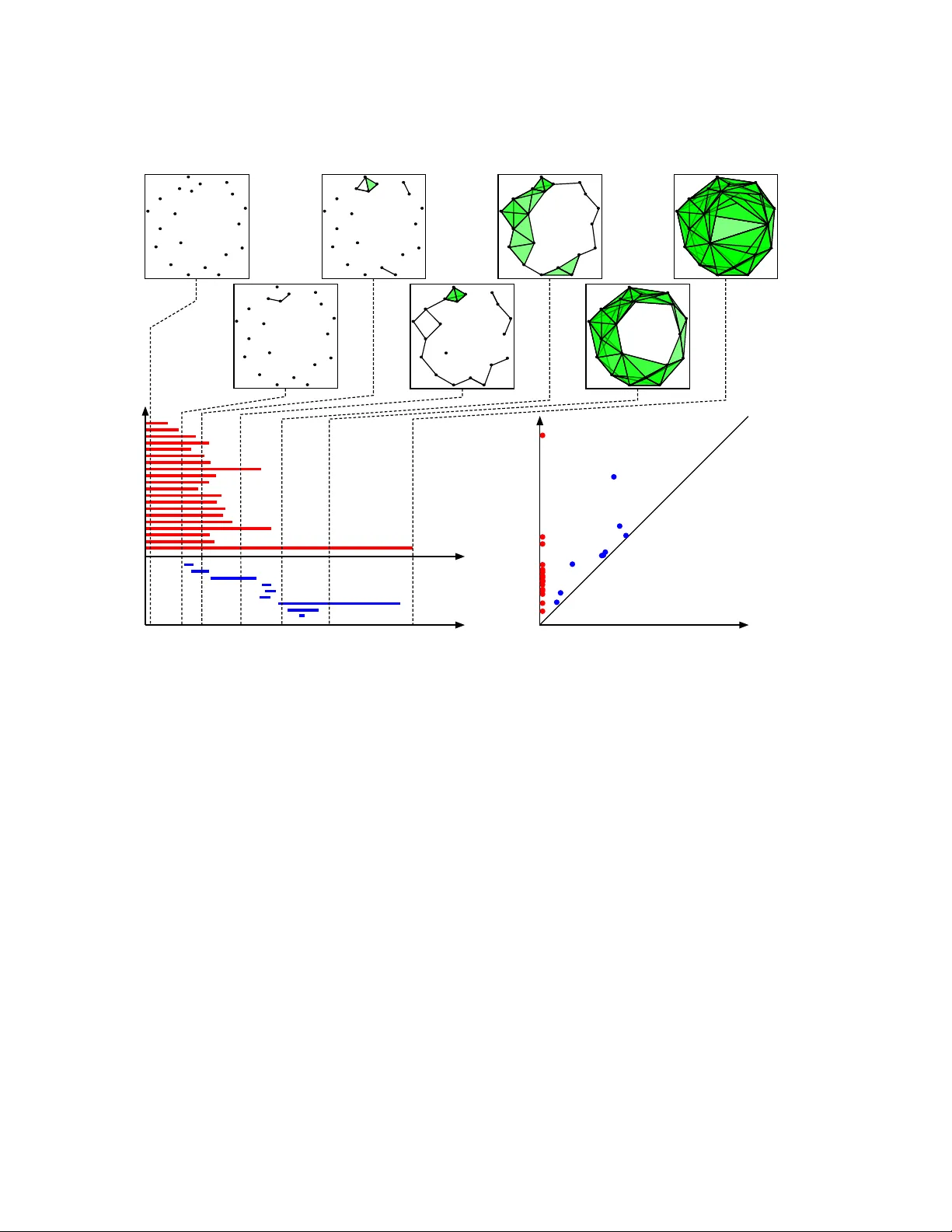
ST A TISTICAL METHODS IN TOPOLOGICAL D A T A ANAL YSIS F OR COMPLEX, HIGH-DIMENSIONAL D A T A P A TRICK S. MEDINA & R.W. DOER GE Abstract. The utilization of statistical metho ds an their applications within the new field of study kno wn as T op ological Data Analysis has has tremendous potential for broad- ening our exploration and understanding of complex, high-dimensional data spaces. This pap er provides an in tro ductory ov erview of the mathematical underpinnings of T op o- logical Data Analysis, the workflo w to con vert samples of data to topological summary statistics, and some of the statistical methods developed for performing inference on these top ological summary statistics. The in tention of this non-tec hnical ov erview is to motiv ate statisticians who are in terested in learning more ab out the sub ject. 1. Introduction Supp ose one is asked to analyze the sample data in Figure 1. What could b e said? Ob vi- ously , it is tw o dimensional, and it app ears to b e circular. How ev er, it ma y b e that these data w ere sampled from a distribution whose supp ort is in the shap e of a circular coil. T ow ard this end, how could a sample of data p oints b e used to study the ov erall shap e of the supp ort of the distribution from which they were sampled? F urthermore, is it p ossible to learn this if these data are high-dimensional? Figure 1. A random sample of 20 p oints sampled from some distribution F with unknown supp ort X ⊆ R n . P A TRICK S. MEDINA & R.W. DOERGE ( a ) ( b ) ( c ) b 0 = 1; b 1 = 0 b 0 = 1; b 1 = 1 b 0 = 1; b 1 = 2; b 2 = 1 Figure 2. Three different mathematical spaces and their Betti n umbers. Betti n um b ers quan tify the distinct num b er of shape features that app ear in a mathematical space. Sp ecifically , connected comp onen ts are H 0 , lo ops b y H 1 , v oids b y H 2 , and so on for higher dimensional analogues. (a) The image of a disc embedded in R 2 . If any t w o p oints are c hosen in the disc then a line may b e drawn connecting the tw o p oints. Hence, there is one connected component and the Betti n um b er for H 0 , β 0 is one. F urther, since there are no holes in the disc then the Betti num ber for H 1 , β 1 is one. (b) The image of a circle em b edded in R 2 . If any t w o points are c hosen along the circle then they may b e connected b y an arc b etw een them. Also, there is a large hole inside of the circle. Hence, β 0 and β 1 are one. (c) The image of a T orus embedded in R 3 . If any t w o p oin ts are c hosen along the exterior, then they may b e connected b y dra wing a path b et ween them, hence β 0 is one. A torus has t w o holes: the first is the large one in the center, and the second is seen by cutting the torus in half. Hence, β 1 is t wo. Finally , the inside of the torus is hollo w, which means it has one void and the Betti n umber for H 2 , β 2 is one. T op ological Data Analysis (TD A) has emerged as a branch of computational top ology that enables researc hers to study the shap e prop erties of a mathematical space based on a representativ e sample tak en from that space. The information is then used to learn how the original mathematical space is organized. TD A uses ideas from algebraic top ology to quan tify distinct shap e characteristics of mathematical spaces. These concepts are general enough that they extend to data that are high-dimensional and very complex; i.e. they reside in spaces where traditional linear statistical methods or manifold learning tec hniques ma y fail to adequately capture prop erties of the underlying space. In the con text of a statistical problem, it is assumed that a sample of data P is dra wn randomly from some distribution F whose supp ort, X ⊆ R n , is unknown. Based on this setting, tour motiv ation is to provide statisticians with a v ery friendly introduction to the mathematical underpinnings of T op ological Data Analysis. Sp ecifically , w e provide an o verview of the pro cess by whic h data, P , are conv erted to differen t top ological sum- mary statistics. The statistical m etho ds dev elop ed for inference on a sample of topological summary statistics are introduced. Finally , the application of some of these statistical metho ds in analyzing differences b etw een t wo structures of the maltose binding protein are examined. ST A TISTICAL METHODS IN TOPOLOGICAL D A T A ANAL YSIS 2. O ver view of Topological Da t a Anal ysis TD A com bines methods from the fields of algebraic top ology and computational geometry for the purp ose of studying key shap e features of a mathematical space from which a sample of data may hav e been dra wn. Tw o k ey to ols for ac hieving this are homology and simplicial complexes. 2.1. Homology. Homology is a sub ject in algebraic top ology that pro vides tools for com- puting the num b er of distinct shap e features within a mathematical space. The shap e features of in terest are connected comp onents - notated by H 0 , lo ops - notated b y H 1 , v oids - notated b y H 2 , and their higher dimensional analogues. F or each of these shap e features a Betti n um b er quantifies the distinct n um b er of shape features that appear in a mathematical space [1]. An example of different mathematical spaces and their Betti n umbers is illustrated in Figure 2. Specific details on homology can b e found in Munkres [2]. Betti n um b ers are t ypically used to understand the shape c haracteristics of a mathematical space. Ho wev er, since data are a collection of discrete p oints, using the data directly as a representation of the underlying mathematical space will not, in general, capture in teresting features that ma y exist. Hence, in order to learn ab out the shap e features of the mathematical space, a geometric representation, known as a simplicial complex, of the space needs to b e constructed from the data. 2.2. Simplicial Complexes. The main to ol for constructing a geometric representation of a mathematical space from data is the simplicial complex. These are topological structures constructed b y attaching simplices along their faces. A simplex is a general te rm for triangles in a Euclidean space. The 0-simplex, or v ertex, is a p oint. The 1-simplex is a line segmen t. The 2-simplex is a triangle. Higher dimensional equiv alen ts of these ob jects follow directly . Examples of the first three simplices are illustrated in Figure 3. Computational metho ds ha v e b een dev elop ed to construct a simplicial complex using a sample of data as the vertices. The details of simplicial complexes can b e found in Munkres [2]. 2.2.1. Computational metho ds for c onstructing simplicial c omplexes. One of the most com- mon approaches for constructing a simplicial complex is the Vietoris-Rips complex [3]. It is constructed b y examining all pairwise distances betw een p oints, P = { p 1 , p 2 , . . . , p n } . Since the data are from a subset X ⊂ R n , numerous notions of distance can b e used. Two common metrics are the p -distance, d p ( x, y ) =  n X i =1 | x i − y i | p  1 p , and the maximum distance, d ∞ ( x, y ) = max n | x 1 − y 1 | , | x 2 − y 2 | , . . . , | x n − y n | o . P A TRICK S. MEDINA & R.W. DOERGE 0-Simplex 1-Simplex 2-Simplex Figure 3. Examples of the first three simplices. The 0-simplex embedded in R is a p oint. The 1-simplex embedded in R 2 is a line segemen t. The 2-simplex embedded in R 3 is a triangle. When p = 2, the p -distance is the Euclidean distance that is used in man y applications, suc h as regression. While these metrics are commonly used in the construction of the complex, other metrics may certainly b e considered. The Vietoris-Rips complex is most easily understo od b y considering a sub collection of p oin ts of τ = { p i 1 , . . . , p i m } ⊆ P . τ is a simplex in the simplicial complex if the p oints are all relatively close to each other. Sp ecifically , the concept of closeness is conceived via a fixed scale parameter  > 0, and τ is a simplex in the simplicial complex if d ( p i j , p i k ) <  for all i j and i k . Once this complex is constructed, it is p ossible to use the to ols dev elop ed from homology to compute the num b er of distinct shap e features presen t. 2.2.2. Cho osing an appr opriate sc aling p ar ameter. F or a fixed v alue of  , the Vietoris-Rips complex is an approximation of the underlying structure. As  increases, more simplices are added to the simplicial complex, until it contains all p ossible simplices that can b e generated from P . Because of the dep endency on the different v alues of the scale parame- ter, information ab out the shap e of the underlying mathematical space v aries, see Figure 4. Instead of using a specific scale parameter  , T op ological Data Analysis uses a range of scale parameters to dynamically keep track of when distinct shap e features appear and disapp ear from the simplicial complex. The concept is similar to the idea of hierarchical clustering, which tracks cluster membership ov er a specified scale parameter, and is kno wn in TDA as “p ersistent homology .” 2.3. P ersisten t Homology. As mentioned, p ersisten t homology [4] tracks the app earance and disappearance of distinct shape features in a simplicial complex via a changing scale parameter. It allows users to understand the n um b er of features that appear in their data, ST A TISTICAL METHODS IN TOPOLOGICAL D A T A ANAL YSIS e =0 e =0.25 e =0.50 e =0.75 e =1.00 e =1.25 e =1.25 Figure 4. The ev olution of the simplicial complex at different v alues of the scaling parameter. As the scaling parameter increases, more simplices are added to the simplicial complex. but also, it ev aluates ho w long these features exist. The details of p ersistent homology ma y be found in Edelsbrunner et al. [4] and Edelsbrunner and Harer [5]. Reviews of the T op ological Data Analysis workflo w may b e found in Carlsson [1], Ghrist [6], and Nanda and Sazadanovi ´ c [7]. 3. Topological Summar y St a tistics T op ological summary statistics allow the quantification and visualization of p ersisten t ho- mology . The main summary statistics used in T op ological Data Analysis are the p ersistence diagram, barco de, and the p ersistence landscap e. Persistence diagrams and barco des are closely related and, as such, the fo cus here will be on the p ersistence diagram and p ersis- tence landscap e. 3.1. The P ersistence Diagram. Persisten t homology tracks the existence of distinct shap e features o ver a range of v alues for a scaling parameter. If a shap e feature app ears at a parameter v alue of  a , and disapp ears at a parame ter v alue of  b , then then the p ersistence diagram retains this information through the point (  a ,  b ) in R 2 . The length of the shap e feature’s existence can b e measured by the v ertical distance b et w een this p oin t and the diagonal ( y = x ). Hence, a persistence diagram is a multiset (a set that allo ws the n um b er of elements to b e rep eated) of p oin ts in R 2 , and the diagonal, where the diagonal has infinite m ultiplicit y . Figure 8 illustrates a p ersistence diagram and explains its in terpretation. Details and metho ds for computing p ersistence diagrams are cov ered in Edelsbrunner and Harer [5]. P A TRICK S. MEDINA & R.W. DOERGE 3.1.1. Mathematic al pr op erties of the p ersistenc e diagr am. In order to make the space of p ersistence diagrams amenable to statistical inference, the definition of a p ersistence dia- gram is limited to a finite m ultiset of p oints in R 2 , and the diagonal ( y = x ), where eac h p oin t on the diagonal has infinite m ultiplicit y [8]. The set of p ersistence diagrams that satisfy this definition, D , equipp ed with the W asser- stein metric is considered a metric space. The p th W asserstein distance b etw een tw o p er- sistence diagrams d 1 , d 2 ∈ D is defined as W p ( d 1 , d 2 ) :=  inf γ X x ∈ d 1 || x − γ ( x ) || p ∞  1 p , where γ v aries across all one-to-one and onto functions from d 1 to d 2 . When D is restricted to the set of p ersistence diagrams whose p th W asserstein distance from itself to the diagonal is finite, Mileyko et al. [8] sho w that the space of previous p ersistence diagrams is a Polish space [9]. This result gives rise to the statistical construct of a mean and v ariance for p ersistence diagrams (see Section 4.1). 3.1.2. Comp arison to the b ar c o de. Persistence diagrams are closely related to the summary statistic referred to as the barco de [10]. A barco de is simply a multiset of in terv als (  a ,  b ) in R 2 , with  a <  b , that keeps track of the app earance and disapp earance of shap e fea- tures across different scaling parameters. Although the barco de is similar to that of the p ersistence diagram it do es not require information ab out the diagonal. Metrics and other prop erties of barcodes may b e found in Carlsson et al. [11], and Zomorodian and Carlsson [12]. An example of how barco des are constructed is found in Figure 8. 3.2. P ersistence Landscap es. P ersistence landscap es are a new concept [13] and are an alternativ e measure of p ersistent homology . P ersistence landscap es, while a statistic, in fact resides in a nicer mathematical space than p ersistence diagrams. As such, they are more amenable to existing statistical methods (fully discussed in Section 4.4). The in terpretation of the p ersistence landscape is more subtle than the in terpretation of either the persistence diagram and the barco de. Rather than directly enco ding information ab out the n um b er of shap e features in a homology group and their length of existence, the persistence landscap e giv es a measure of the num ber of features that sim ultaneously exist at a particular scaling parameter. An example of a p ersistence landscap e is in Figure 5. 3.2.1. Mathematic al pr op erties of a p ersistenc e landsc ap e. A p ersistence landscap e, Λ, is a sequence of piecewise con tin uous functions λ k : R → R . Distance measures may b e defined for p ersistence landscap es b y integrating the functions, λ k , and summing the result across all v alues of k . P ersistence landscap es can b e treated as a random v ariable that tak es v alues in a Banac h space, whic h gives rise to the use of probabilistic results [14]. Details and other results are co vered in Bub enik [13]. ST A TISTICAL METHODS IN TOPOLOGICAL D A T A ANAL YSIS − 4 − 3 − 2 − 1 0 1 − 4 − 3 − 2 − 1 0 1 x1 x2 0.0 0 0.0 5 0.1 0 0.1 5 0.2 0 0.0 0 0.0 2 0.0 4 0.0 6 0.0 8 Per sistence Landscape Tim e λ λ (3) λ (2) λ (1) Figure 5. Left: A random sample of 200 points uniformly dra wn from t w o differen t circles; 100 p oints w ere sampled from the circle cen tered at (0 , 0) and 100 p oints were uniformly sampled from the circle centered ( − 3 , − 3). F or these samples the Betti num bers for the connected comp onents and holes are b oth t wo. Right: The p ersistence landscap e for the num ber of connected comp onents. The p ersistence landscap es are such that λ 1 ≥ λ 2 ≥ · · · ≥ λ n . Since the first tw o p ersistence landscap es are large, this giv es evidence for the num ber of connected comp onents b eing t w o, whic h is consisten t with the example on the left. 4. St a tistical Inference with Topological Summar y St a tistics A significant amount of work has b een performed for the purp ose of extending statistical metho ds to T op ological Data Analysis. W e are sp ecifically interested in defining a clear notion of the mean and v ariance for p ersistent homology , developing testing metho ds that distinguish b et ween the distributions from which top ological summary statistics may hav e b een sampled, and metho ds for determining which shap e c haracteristics are statistically significan t and whic h are top ological noise. Here, w e review some of the statistical metho ds dev elop ed for b oth the p ersistence diagram and the p ersistence landscap e. It is generally assumed that the p oints of the sample P = { X 1 , . . . , X n } ⊆ R n are identi- cally and indep endently distributed through some random pro cess with distribution F X . Applying the T op ological Data Analysis workflo w to P results in a top ological summary statistic, T S ( P ). Ho wev er, the distribution of our topological summary statistic ma y not follo w the same distribution as the original sample. Hence, in order to understand the distribution of the top ological summary statistic it is necessary to understand the effect of the top ological transformation on the distribution of the original data. As a simple ex- ample of this effect, supp ose U is a random sample drawn from Uniform(0 , 1) distribution, P A TRICK S. MEDINA & R.W. DOERGE then − ln( U ) is distributed as an exp onential(1) random v ariable. In general, it is not clear what influence the top ological transformation has on the distribution of the data. 4.1. F r ´ ec het mean and v ariance of p ersistence diagrams. The F r´ ec het mean and v ariance of p ersistence diagrams are discussed in [8]. Let ( D P , B ( D P ) , F D P ) b e a probability space on the space of p ersistence diagrams as defined in Section 3.1.1, where B ( D P ) is the Borel σ -algebra on D P , and F D P is a probabilit y measure on this space. In order to define the F r´ ec het mean it is required that F D P ha ve a finite second moment. That is, M D P ( d ) = Z D P W p ( d, e ) d F D P ( e ) < ∞ , for a fixed diagram d ∈ D P . The F r´ ec het v ariance is defined as V ar F D P := inf d ∈D P n M D P ( d ) < ∞ o , and the F r ´ echet mean by E F D P := n d | M D P ( d ) = V ar F D P o . Since the definition of a F r ´ echet mean is an infimum ov er a space, in general, the mean ma y not b e unique. T o our knowledge, this is the only definition of a mean and v ariance for p ersistence landscap es. 4.1.1. A lgorithm for c omputing the F r ´ echet me an and varianc e. An algorithm for comput- ing the F r ´ ec het mean is giv en in T urner et al. [15] for the special case of the L 2 -W asserstein metric and the distribution of the sample of p ersistence diagrams is a com bination of Dirac masses [16]. In this setting, the authors provide a law of large num b ers, how ev er they can only ensure that their algorithm conv erges to a lo cal minim um. 4.2. Hyp othesis T esting for P ersistence Diagrams. A problem of particular in ter- est in T op ological Data Analysis is determining whether t w o subsets of R n are the same. Robinson and T urner [17] present an argument that a necessary , but not sufficien t, con- dition is that the underlying distribution of their p ersistence diagrams are the same. T o accomplish this, they dev elop a nonparametric p ermutation test to test for differences in the distributions of tw o differen t samples of p ersistence diagrams. Rejecting a n ull hypoth- esis, H 0 , that the tw o distributions are the same provides evidence that the tw o subsets, themselv es, are different. Details of the joint loss function that is emplo y ed, the reasons for dev eloping a p ermutation test, and the justification for the output of their metho d being a p -v alue are in Robinson and T urner [17]. ST A TISTICAL METHODS IN TOPOLOGICAL D A T A ANAL YSIS 4.3. Confidence Sets for Persistence Diagrams. As with the ma jority of statistical applications, there is an in terest in separating signal from noise. As such, an in teresting question in p ersisten t homology is how to distinguish imp ortant shap e features from top o- logical noise. The general working h yp othesis in T op ological Data Analysis is that features whic h exist (i.e., persist) ov er large interv als of the scaling parameter are significant. How- ev er, it is not alwa ys clear what constitutes a large in terv al, or if features that exist o ver a small interv al are truly noise or of in terest. This first issue is addressed by F asy et al. [18] who originated metho ds for computing a 1 − α confidence set for an estimated p ersistence diagram. F or instance, supp ose P is a single sample tak en from some distribution F , then a p ersistence diagram ˆ d ma y b e constructed from the data. A v alue, c n , is computed from the data so that when the v ertical distance b etw een a p oint and the diagonal is less than √ 2 c n the lifespan of the feature is not different from zero. 4.4. P ersistence Landscap es. P ersistence landscap es that are assumed to b e random v ariables that take v alues in a Banach space are more amenable to the classical statistical theory of h yp othesis testing and confidence in terv als. In Bub enik [13] the vector space structure of the underlying L p space is used to construct a p oint wise mean for the p ersis- tence landscap e Λ. That is, if we hav e samples P 1 , . . . , P n , with corresp onding p ersistence landscap es Λ 1 , . . . , Λ n , then the mean landscap e for the k th sequence is given by ¯ λ k ( t ) = 1 n n X i =1 λ i k ( t ) . Using results from [14], Bub enik [13] shows that the Strong Law of Large Num bers holds for the mean persistence landscap e and that they obey the Central Limit Theorem. Chazal et al. [19] show that the con v ergence of the Central Limit Theorem is uniform. 4.4.1. Hyp othesis testing for p ersistenc e landsc ap es. An adv antage of the p ersistence land- scap e is that it allows for hypothesis testing when samples are high-dimensional and non- linear. In order to use p ersistence landscap es for hypothesis testing one has to use a functional - functions that map R n to R - on the p ersistence landscap es. When function- als satisfy certain conditions, Bub enik [13] pro ved the Central Limit Theorem remains for the transformed p ersistence landscap e. Under this framew ork classical hypothesis testing pro cedures exist, and can b e emplo y ed to distinguish betw een ob jects. In other w ords, for a large num ber of samples, it is p ossible to use common t -tests or Hotelling’s T 2 to distinguish b et w een t w o subsets of R n . It should b e noted that applying a functional in fact, pro jects all of the information in a p ersistence landscape to a single p oint. While this may result in a loss of information, this approac h mak es it easier to directly apply classical statistical tests, suc h as the t -test. P A TRICK S. MEDINA & R.W. DOERGE 1OMP (open- apo conformation) 1MPD (closed- holo conformation) H 0 H 1 H 2 H 0 H 1 H 2 Figure 6. Barco des for the first three homology groups of the closed con- formation structure (left) and the op en conformation structure (right) [20]. Sligh t differences b et w een the tw o structures can b e seen in the first ho- mology group. Differences b etw een the other homology groups are more subtle. 5. Applica tion of Topological Da t a Anal ysis f or Studying the Conforma tion Sp ace of the Mal tose Binding Protein T echnologies exist to capture proteins in a w a y that enables the study of their physical structure in three-dimensional space. Ho w ever, when a protein is captured its physical structure represents one of man y p ossible shap es. Many factors, including en vironmen tal or biological function, ma y influence the ov erall shap e of a protein. Kov acev-Nik olic et al. [20] consider the conformation space, or the space of possible shapes, of the maltose binding protein was studied using top ological metho ds. It is kno wn that the maltose binding protein mak es conformational c hanges when a ligand attaches. If a protein is closed it is alwa ys prone to ha ving a ligand attac hed. One ob jectiv e of Kov acev-Nikolic et al. [20] w as to determine if statistically significan t differences exist b et w een the structures of the open and closed conformation space. A sample of seven open structures and sev en closed structures were obtained from the protein data bank [21]. The proteins were conv erted from their physical co ordinates to a structure that considers the energy relationship b et w een residues using the elastic netw ork mo del. Reasons for this conv ersion are discussed in [20]. Persisten t homology is then computed on each sample using the Vietoris-Rips complex, discussed in Section 2.2.1. Figure 6 illustrates one of the computed barco des for the first three homology groups, and Figure 7 illustrates the mean p ersistence landscap es for the first tw o homology groups. In order to p erform a h yp othesis test, a functional is applied to eac h p ersistence landscap e, resulting in a single v alue (1) X j i,h = ∞ X k =0 Z R λ k ( t ) dt , ST A TISTICAL METHODS IN TOPOLOGICAL D A T A ANAL YSIS H 1 H 0 Open Closed Figure 7. Persistence landscap es for the num b er of connected comp onents, H 0 (top) and holes, H 1 (b ottom) for the closed conformation structure (left) and the op en conformation structure (righ t) [20]. (top) Observ able differences b et ween the closed and op en p ersistence landscap e are observ ed in the first homology group, H 0 . The second p ersistence landscap e of the closed structure attains a peak v alue of more than 0 . 30 and attains that v alue at ab out 0 . 40, while the second p ersistence landscap e of the op en structure attains a p eak v alue at around 0 . 20 and attains that v alue at ab out 0 . 30. F or the first homology group, H 1 , the initial p eak of the first few p ersistence landscap es of the closed structure are uneven, while the same p ersistence landscap es in the op en s tructure are smo oth. where 1 ≤ j ≤ 7, i ∈ { op en , closed } , and 0 ≤ h ≤ 2 is the homology group. This functional is simply the total area area under all of the p ersistence landscap es in the k th homology group. Using these v alues, a permutation test is p erformed to compare the mean v alue of eac h homology group H 0 : µ h, op en = µ h, closed against H a : µ h, op en 6 = µ h, closed . The p -v alues for homology in b oth degree zero and one were computed to b e 5 . 83 × 10 − 4 giving evidence of a significan t difference in the n um b er of connected components and holes, while the p -v alue for the second homology group is 0.0396. No corrections on the significance lev el w ere considered for multiple-testing, ho wev er the p -v alues for homology in degree P A TRICK S. MEDINA & R.W. DOERGE zero and degree one are small enough to conclude differences in the means exist for these homology groups. 6. Discussion Impro vemen ts in biotec hnology ha v e resulted in a massiv e gro wth of the amount and com- plexit y of the data used in ev ery field. In this w ork we ha v e introduced the untapped p o wer of tools pro vided by T op ological Data Analysis. The TDA framework is well sit- uated for studying datasets that are high-dimensional and complex. Although there is evidence of success in applying these metho ds to b oth visualize high dimensional data and for classification, further extensions of statistical metho ds to T op ological Data Analysis are needed. ST A TISTICAL METHODS IN TOPOLOGICAL D A T A ANAL YSIS (a) (b) Scaling+Paramet er H0 H1 Figure 8. The top of the plots represen t the simplicial complex at different v alues of the scaling parameter. (a) Illustration of the barco de summary statistic. The red and blue bars show the p ersistent homology of the con- nected components, H 0 , and lo ops, H 1 , resp ectively . The x -axis is the scaling parameter. At each v alue of the scaling parameter the num b er of distinct features that exist ma y b e counted for each homology group by simply counting the n um b er of bars at that v alue. F or example, for the first simplicial complex there are tw en t y connected comp onents and zero holes since the complex is starting with tw en ty v ertices. At the fourth simplicial complex there are three connected comp onents and one hole. The length of each bar indicates the length of each shap e feature’s existence. (b) Il- lustration of the p ersistence diagram. The red and blue dots indicate show the p ersistent homology of the n um b er of connected comp onents and holes resp ectiv ely . F or each dot, the x -co ordinate indicates the v alue of the scal- ing parameter at which the shape feature app eared and the y -co ordinate indicates the v alue of the scaling parameter at which the shap e feature dis- app eared. The distance from eac h p oin t to the diagonal indicates the length of each shap e feature’s existence. Since all features in H 0 existed at time zero, they are all ab ov e the p oin t x = 0. The features for H 1 came into existence at later times, so they are scattered at differen t p oin ts in the x -axis. P A TRICK S. MEDINA & R.W. DOERGE References [1] Gunnar Carlsson. T op ology and data. Bul letin of the Americ an Mathematic al So ciety , 46(2):255–308, 2009-04. [2] James R. Munkres. Elements of Algebr aic T op olo gy . Perseus, Reading, MA, 1984. [3] Afra Zomorodian. F ast construction of the vietoris-rips complex. Computer and Gr aphics , page 263271, 2010. [4] Letsc her, D. Edelsbrunner, H. and Zomoro dian, A. T op ological persistence and simplification. Discr ete & Computational Ge ometry , 28(4):511–533, 2002. [5] Herbert Edelsbrunner and John Harer. Computational T op olo gy: An Intr o duction . American Mathe- matical So ciet y , 2010. [6] Robert Ghrist. Barco des: The p ersistent top ology of data. Bul letin of the Americ an Mathematic al So ciety , 45(1):61–75, 2008-01. [7] Vidit Nanda and Sazadanovi ´ c Radmila. Simplicial models and topological inference in biological sys- tems. In Nata ˇ sa Jonosk a and Masahico Saito, editors, Discr ete and T op olo gic al Mo dels in Mole cular Biolo gy , Natural Computing Series. Springer Berlin Heidelb erg, 2014. [8] Y uriy Mileyko, Say an Mukherjee, and John Harer. Probability measures on the space of persistence diagrams. Inverse Pr oblems , 27(12):124007, 2011. [9] Ric hard M. Dudley . Elements of A lgebr aic T op olo gy . Chapman & Hall, New Y ork, NY, 1989. [10] Anne Collins, Afra Zomoro dian, Gunnar Carlsson, and Leonidas Guibas, J. A barco de shap e descriptor for curv e p oint cloud data. Computer & Gr aphics , 28:881–894, 2004. [11] Gunnar Carlsson, Afra Zomoro dian, Anne Collins, and Leonidas J. Guibas. Persistence barco des for shap es. International Journal of Shap e Mo deling , 11(2):149–187, 2005. [12] Afra Zomoro dian and Gunnar Carlsson. Computing p ersistent homology . Discr ete Computational Ge- ometry , 33:249–274, 2005. [13] P eter Bub enik. Statistical topological data analysis using persistence landscapes. Journal of Machine L e arning R ese ar ch , 16:77–102, 2015-01. [14] Mic hel Ledoux and Michel T alagrand. Pr ob ability in Banach Sp ac es . Classics in Mathematics. Springer- V erlag, 2011. [15] Katharine T urner, Y uriy Mileyko, Sa yan Mukherjee, and John Harer. F r´ ec het means for distributions of p ersistence diagrams. Discr ete & Computational Ge ometry , 52(1):44–70, 2014-07. [16] Jean Dieudonne. T r e atise on Analysis, V olume 2 . Pure and Applied Mathematics (Book 10). Academic Press, 1976. [17] Andrew Robinson and Katharine T urner. Hyp othesis testing for top ological data analysis. arXiv pr eprint arXiv:1310.7467 , 2013. [18] Brittan y T. F asy , F abrizio Lecci, Alessandro Rinaldo, Larry W asserman, Siv araman Balakrishnan, and Aarti Singh. Confidence sets for p ersistence diagrams. The Annals of Statistics , 42(6):2301–2339, 2014. [19] F rederic Chazal, Brittany T. F asy , F abrizio Lecci, Alessandro Rinaldo, and Larry W asserman. Stochas- tic con vergence of p ersistence landscap es and silhouettes. arXiv:1312.0308 [math.ST] . [20] Violeta Kov acev-Nikolic, Peter Bub enik, Dragan Nikolic, and Giseon Heo. Using cycles in high dimen- sional data to analyze protein binding. eprint , page 21, 2014-12. [21] F. C. Bernstein, T. F. Ko etzle, G. J. Williams, E. F. Mey er, M. D. Brice, J. R. Ro dgers, O. Ken- nard, T. Shimanouchi, and M. T asumi. The Protein Data Bank: a computer-based arc hiv al file for macromolecular structures. Journal of mole cular biolo gy , 112(3):535–542, May 1977.