Bayesian isochrone fitting and stellar ages

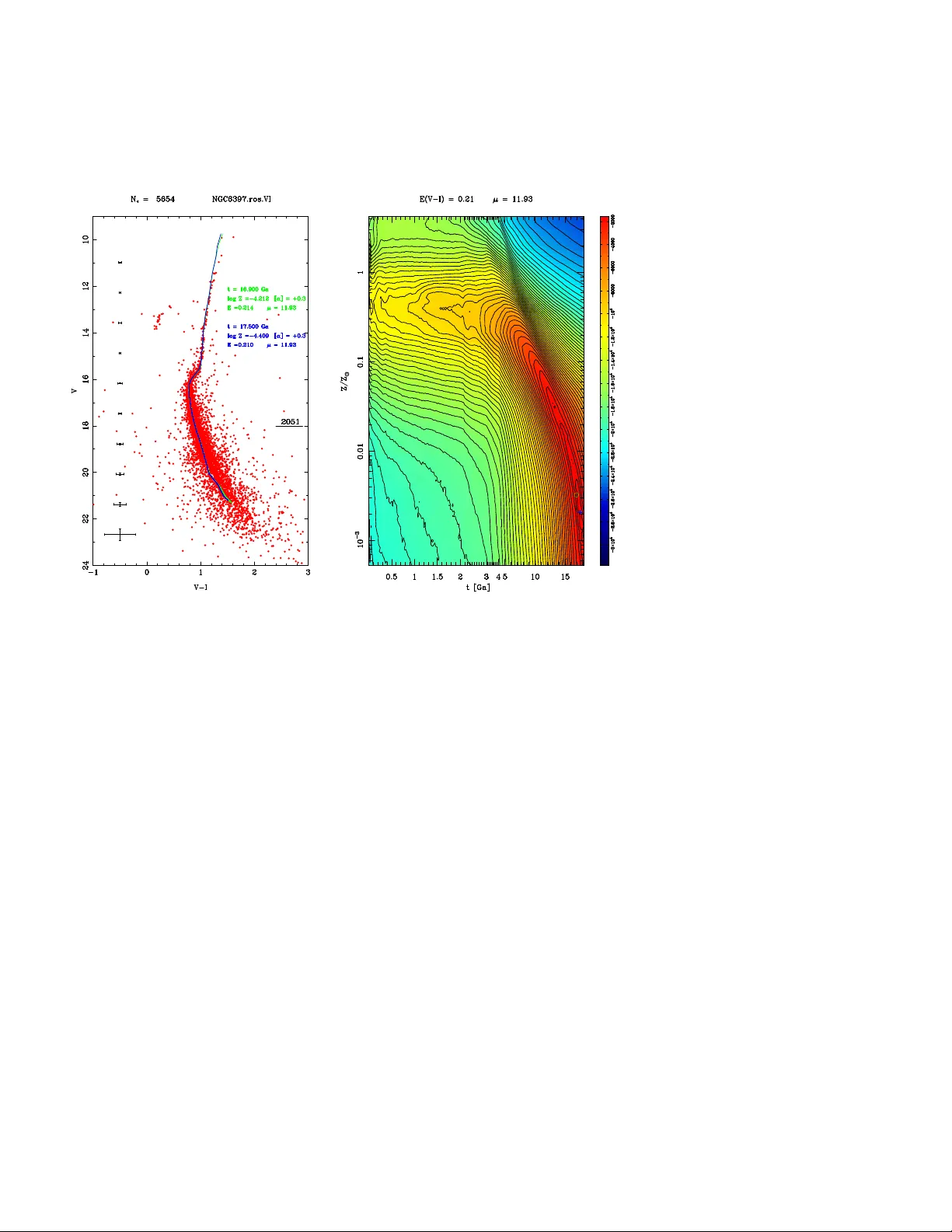
The A ges of the Stars Y. L ebr eton, D. V al ls-Gab aud & C. Charb onnel (e ds) EAS Public ations Series, V ol. 65, 2014 BA YESIAN ISOCHRONE FITTING AND STELLAR A GES Da vid V alls-Gabaud 1 Abstract. Stellar evolution theory has been extraordinarily successful at explaining the diﬀerent phases under which stars form, evolv e and die. While the strongest constrain ts ha ve traditionally come from bi- nary stars, the adv ent of asteroseismology is bringing unique measures in well-c haracterised stars. F or stellar populations in general, how ever, only photometric measures are usually av ailable, and the comparison with the predictions of stellar evolution theory hav e mostly b een qual- itativ e. F or instance, the geometrical shap es of iso c hrones hav e b een used to infer ages of coev al p opulations, but without any prop er sta- tistical basis. In this c hapter w e pro vide a p edagogical review on a Ba yesian formalism to make quantitativ e inferences on the prop erties of single, binary and small ensem bles of stars, including unresolved p opulations. As an example, w e sho w ho w stellar ev olution theory can b e used in a rigorous w ay as a prior information to measure the ages of stars b et ween the ZAMS and the Helium ﬂash, and their uncertain ties, using photometric data only . 1 Intro duction In this chapter a brief summary is presented of the uses of stellar evolution the- ory to infer prop erties of single stars (Section 3 ), of detached binary stars whose comp onen ts are assumed to ha v e ev olv ed independently of each other (Section 4 ), and coev al stellar populations suc h as (presumably) those in clusters (Section 5 ). When the fundamental prop erties of the star(s) in question are known (mass, absolute luminosity , eﬀectiv e temperature, etc), stellar tracks computed for this particular (set of ) star(s) can b e used to infer further prop erties, suc h as ages. In general, how ever, one wishes to use the predictions of stellar ev olution to infer these prop erties. The data at hand are usually magnitudes and colours, hence 1 LERMA, CNRS UMR 8112, Observ atoire de P aris, 61 Av enue de l’Observatoire, 75014 Paris, F rance. Email david.valls- gabaud@obspm.fr c  EDP Sciences 2016 DOI: (will b e inserted later) 2 The Ages of the Stars the interpretation of the features in the colour-magnitude diagrammes (CMDs) is carried out with isochrones rather than stellar trac ks. The thorny issue of trans- forming iso c hrones from/to the theoretical diagram to/from observ ed CMDs will not b e dealt with here (see the contributions b y Cassisi, and b y Lebreton, Goupil and Montalb´ an in this volume), and constitute one of the sources of systematic uncertain ties. One also has to b ear in mind that while many eﬀorts ha ve b een placed to ﬁnd the b est transformations, the diﬀerences observed cannot (yet?) b e fully ascribed to either systematics in the observ ations or in missing/wrong physics in the stellar evolutionary calculations. F or instance the recent analysis by V an- denBerg et al. ( 2010 ) for some globular clusters, and by An et al. ( 2007 ) for op en clusters show that while some CMDs can b e w ell ﬁtted, other colour-magnitude com binations of the same clusters show anomalies which go w ell b ey ond the cor- rections for systematics, rotation, activity , transformations, metallicit y , etc. Em- pirical b olometric corrections are another source of uncertain t y ( T orres , 2010 ) as are the systematics in the determination of eﬀective temperatures ( e.g. , Ram ´ ırez & Mel´ endez , 2005 ). Likewise, it does make sense to adopt a standard set of v alues ( Harmanec & Pr ˘ sa , 2011 ) with nominal v alues to a void some of the systematics arising with the adoption of diﬀeren t k ey v alues (solar radius, mass, etc). Section 6 deals with the general problem of in verting the CMDs of a mixture of resolv ed stel- lar populations to infer their distribution of ages and hence their c hemical and star formation rate histories, while Section 7 is a very brief discussion on CMDs of pix- els in unresolv ed stellar populations. Section 8 closes this chapter with a discussion on some statistical issues in the in terpretation of CMDs. W e will limit the scop e of this c hapter to stars from the main sequence to the Helium ﬂash, as the pre- dictions in this range app ear to b e the most robust ones. The white dw arf phase can also b e used in a rather robust w ay (provided the co oling and the equation of state are prop erly characterised), as describ ed by T. von Hipp el in this volume. 2 Colour-Magnitude and Hertzsp rung-Russell Diagrammes The plotting of the colors (or spectra) of stars as abscissae against their absolute magnitudes (total magnitudes) has b ecome one of the most lucrativ e adven tures in the study of star light. Shapley ( 1960 ) It is appropriate to recall, in the con text of this v olume, that just o ver a century ago the ﬁrst colour-magnitude diagram (CMD) was published. The author of this landmark pap er was not Ejnar Hertzsprung nor Henry N. Russell, but Hans O. Rosen b erg, a colleague of Karl Sch warzsc hild at G¨ ottingen. Rosenberg had b een w orking since 1907 on getting sp ectral prop erties of stars b y measuring plates ob- tained with the Zeiss ob jectiv e prism camera ( Hermann , 1994 ). T o maximise the n umber of sp ectra per plate, he observed the Pleiades cluster and obtained sp ectra D. V alls-Gabaud: Ba yesian Iso chrone Fitting 3 for ab out 60 of them, ov er 1907–1909, noting that their inferred eﬀective temp er- atures correlated with their apparen t magnitudes in the ﬁrst ever published CMD ( Rosen b erg , 1910 ) 1 . His goal was to “ make the most accurate determination of the sp ectral t yp es of stars in the Pleiades ” by using a “ physiological blend ” of the depth and width of the Ca ii K line (393.37 nm) with the Balmer H δ and H ζ lines. He excluded the Ca ii H line at 396.9 nm as it w as blended with H  in the very lo w disp ersion sp ectra he used (1.9 mm from H γ to H ζ ). With an exp osure time of 90 min utes he could measure sp ectra down to the 10th photographic magnitude, ﬁnding that for the actual members of the Pleiades “ there is a strict relation b e- t ween the brightness and the sp ectral type, with no exception in the interv al from the 3rd to the 9th magnitude. ”. Hertzsprung’s diagrams (magnitude vs colour) of the Pleiades and the Hyades would app ear a year later ( Hertzsprung , 1911 ) while Russell’s version for ﬁeld stars with parallaxes (with absolute magnitude vs sp ec- tral type) w ould only app ear in 1914 ( Russell , 1914a , b ), although the correlation b et ween luminosity and sp ectral type was noted by Hertzsprung in 1905 and in more detail by Russell ( 1912 ). The key diﬀerence is that while Russell required parallaxes to ascertain the distances to the stars, Rosenberg carefully chec ked the mem b ership of stars in the Pleiades, rejecting outliers and non-members. Henry Russell was obsessed by priority , (self-)attribution and promotion ( De- V orkin , 2000 ). F or example, the famous V ogt(–Russell) theorem on stellar struc- ture ﬁrst app eared in 1926 ( V ogt , 1926 ) and in his inﬂuential textb ook Russell do es give full credit to V ogt ( Russell, Dugan & Stewart , 1927 ), yet he will later claim ( Russell , 1931 ) that he had found it indep endently . In the case of the CMD, Russell called it in priv ate the “Russell diagram”, but this w as not accepted in pub- lic, as the con tribution by Hertzsprung (unlike Rosenberg’s) was well and widely kno wn. Russell p oured ov er the astronomical journals, and w as well a ware of Hertzsprung’s results. W e know he read the Astronomischen Nachric hten system- atically , as one of the leading journals of the time, and that we was well aw are of Hertzsprung’s pap ers just as was his mentor, E.C. Pick ering, who received them and wrote to Hertzsprung discussing several issues in sp ectral classiﬁcation. Rus- sell wrote to Hertzsprung on September 27, 1910, thanking him for sending copies of his papers ( Hearnshaw , 1986 ). Hertzsprung ( 1911 )’s paper contained the CMDs of the Hyades and the Pleiades, citing explicitely the previous –and pioneering– w ork by Rosenberg ( 1910 ). With the raising inﬂuence of European (mosly Dutch) astronomers in the USA, the issue of the prop er ackno wledgemen t b ecame very serious and created frictions and debate within the communit y . After tw o decades, the “Russell diagram” b ecame known as the Hertzsprung-Russell diagram, thanks in part to the inﬂuential conference delivered in 1933 by B. Str¨ omgren at the meeting of the Astronomische Gesellschaft, but muc h to the irritation of many , including Russell himself who ev en refused to ackno wledge that Hertzsprung had found (and coined the terms) ‘gian t’ and ‘dwarf ’ stars ( Smith , 1977 ). The (proper) renaming of the diagram was a long battle which lasted till the late 1940s, when 1 A translation into English is a v ailable at Leos Ondra’s w ebsite www.leosondra.cz/en/first- hr- diagram 4 The Ages of the Stars S. Chandraskhar, advising the Astrophysical Journal and tired of the contro versy , decided that the standard nomenclature would be the “H–R Diagram” ( DeV orkin , 2000 ). Rosen b erg’s pioneering contribution has b een unfairly forgotten from the history describing the elab oration of the ﬁrst CMDs (see, e.g. , W aterﬁeld , 1956 ; Nielsen , 1969 ; DeV orkin , 2000 ). Hans Rosenberg w as b orn in Berlin on May 18, 1879, and studied ﬁrst in Berlin, under W. F o erster, and then in Strasb ourg, with E. Beck er, obtaining his Dr. Phil. with a thesis on the p erio d changes that χ Cygni underwen t from 1686 to 1901. Interested in b oth instrumentation and astrophysics, he mov ed to G¨ ottingen to w ork with Karl Sc hw arzschild where he was to pro duce the ﬁrst large surv ey of stellar temp eratures estimated with ob jetive prism sp ectra. F or years, the Rosenberg temp erature scale will set the standard and will b e widely used, as w ell as his review on photo electric photometry in the Handbuch der Astrophysik ( Rosen b erg , 1929 ). His Habilitation thesis from T ¨ ubingen in 1910 was on “ The relation b et w een brightness and sp ectral type in the Pleiades ”, whose results were published in the ab ov e-cited key pap er in Astr. Nac h. ( Rosenberg , 1910 ). His instrumen tal exp ertise allow ed him to get sp ectra of comets Daniel (1907 IV) and Morehouse (1908 I I I). F rom 1910 on, he work ed at T ¨ ubingen ﬁrst as Priv atdozent, where he founded its observ atory in ¨ Osterb erg, b ecoming its director in 1912 and professor at the universit y in 1916 while serving in the army during W orld W ar I. He made with P . Go etz the ﬁrst photometric map of the Mo on, and developed the use of photo electric cells as astronomical detectors in 1913. Moving to Kiel in 1925 he work ed on solar eclipses, developed direct measures of the colours of stars and had heavy teac hing duties. In spite of his p osition as professor at Kiel univ ersity , on April 1, 1933, three uniformed members of the feared SA Nazi paramilitary group came to his appartment and forced him to resign ( Duerbeck , 2006 ), but he w ould ha ve lost his p osition all the same with the racial laws enacted in 1935. He was immediately in vited in 1934 by the Universit y of Chicago to work at Y erkes Observ atory where he stay ed three years, working on measures of the lim b darkening and colour indices in eclipsing binaries ( e.g. , Rosenberg , 1936 ). In 1938 he was app oin ted director of Istanbul Observ atory , where he reorganised the teac hing of astronomy at the Universit y of Istanbul and set up new priorities for the observing campaigns. He passed aw a y there on July 26, 1940, a week after suﬀering a heat strok e ( Gleissb erg , 1940 ). An even earlier relationship b et ween the colour and the magnitude was found b y Charlier ( 1889 ), who studied the correlation b et ween magnitude and a colour- lik e quan tity (the diﬀerence b et ween the magnitude he measured in a photographic plate and the visual magnitude) as determined by Max W olf in Heidelb erg. How- ev er, he interpreted the correlation found (the visually fainter stars had larger diﬀerences) as a systematic error in the visual magnitudes. As Rosen b erg cor- rectly p oin ted out, this could also b e pro duced by selective reddening, hence the imp ortance of getting spectra. The sp ectral t yp e – magnitude correlation found in the Pleiades could not be produced by dust, hence “ the plausible colour diﬀerences among the stars in the Pleiades –the fainter the star, the redder it is– following from the optical and photographic brightness measurements are conﬁrmed b y the D. V alls-Gabaud: Ba yesian Iso chrone Fitting 5 sp ectral prop erties ”. This ground-breaking result will b e taken to go o d use to lay the foundations of stellar physics (see, e.g. , Salaris & Cassisi , 2005 ), but the true pioneer has unfairly b een forgotten to the exten t that it w ould b e a ﬁtting trib- ute to rename the diagram as the Rosenberg-Hertzsprung-Russell diagram (RHR). Ironically , HR also stands for Hans Rosenberg’s initials. The ﬁnal word may come from Hertzsprung himself. His mo desty made him to av oid talking ab out his o wn contributions to astronomy , and, as Strand ( 1968 ) reminds us, he remark ed on the con trov erted issue of the naming of the diagram: “ Wh y not call it the colour–magnitude diagram? Then w e know what it is all ab out. ” The use of CMDs to constrain the physical prop erties of the stars was noticed v ery quickly . In fact, Russell ( 1912 ) was the very ﬁrst to use the correlation b et ween absolute magnitude and sp ectral type for (dw arf ) stars with measured parallaxes to infer a distance to the Pleiades of 500 light-y ears 2 . 3 Single stars The ﬁtting of iso c hrones to a set of stars is the main metho d to constrain their ph ysical properties, b esides other techniques which are limited to nearby stars such as stellar oscillations. The set of basic prop erties includes the age t , Helium abun- dance Y , metallicity Z , α elemen ts ov er abundance, distance mo dulus µ = m − M , con vection mixing length, etc, that is, all the quantities which determine the p o- sition of stars in a CMD. In contrast with its imp ortance for stellar evolution, relativ ely little work has b een done to formulate mathematically the problem to go b ey ond the ‘ﬁt-by-ey e’ approach which has characterised this ﬁeld (and unfor- tunately still do es!). It seems that the ﬁrst attempt to ﬁnd the separation of a star from an iso c hrone comes from Schalten brand ( 1974 ) who developed a simple metho d to estimate the nearest p oin t of the zero-age main sequence to a giv en star in a tw o-colour diagram under the assumption of Gaussian errors. This ap- proac h was further formalised in a prop er probabilistic framework by Luri, T orras & Figueras ( 1992 ) as the so-called ‘proximit y parameter’, similar to the determin- istic ‘near p oin t’ estimator b y Flannery & Johnson ( 1982 ). Here one computes the sum of minimum distances from a set of N ? stars to a given iso c hrone with given prop erties (age t , Helium abundance Y , metal conten t Z , etc) along with prop er- ties of the set of stars, which can also b e applied to the theoretical iso chrone, such as the distance mo dulus µ or the extinction. W e represen t this set as the vector of parameters ~ ϑ = ( t, Y , Z, µ, · · · ). One can form the statistic Ψ 2 whic h is calculated 2 The spectra of the fainter mem b ers of the Pleiades came from E.C. Pick ering and A. Cannon, and no men tion is made of Rosenberg ( 1910 )’s work nor the comprehensive survey by Hertzsprung ( 1911 ). 6 The Ages of the Stars as the sum of minimal (squared) distances: Ψ 2 ( ~ ϑ ) = N ? X i =1 min j  d 2 ij  , (3.1) where d ij is the geometrical distance b et ween the observed star num b er i and the theoretical p oin t j of the given iso c hrone: d 2 ij =  m i − m j σ ( m i )  2 +  c i − c j σ ( c i )  2 , (3.2) and m and c are magnitudes and colours resp ectively , or gravities and temp era- tures, or an y tw o observ ables whic h can b e predicted with the mo dels, while σ ( m i ) and σ ( c i ) are the errors in these quan tities for the given star lab eled i . This dis- tance can ob viously b e generalised to an y n -dimensional space (see below). If (and this is a ma jor assumption, see b elow) the mo del stars w ere uniformly distributed along the iso chrone, then the probability that one observed star comes from that iso c hrone would b e P i ( ~ ϑ ) = 1 2 π σ ( m i ) σ ( c i ) N iso X j =1 exp  − d 2 ij / 2  , (3.3) where N iso is the total num b er of p oints the isochrone has b een divided into. The probabilit y that an ensemble of N ? stars comes from an iso chrone with the set of prop erties ~ ϑ is just the pro duct of the individual probabilities P total ( ~ ϑ ) = N ? Y i =1 P i ( ~ ϑ ) . (3.4) One can then use the standard maximum likelihoo d technique to ﬁnd the set of parameters ~ ϑ which maximises this probability . The maxim um lik eliho o d statistic (MLS) w ould for instance b e MLS( ~ ϑ ) = − log P total ( ~ ϑ ) = N ? X i =1 log P i ( ~ ϑ ) . (3.5) F or, say , m = 3 parameters (distance mo dulus, age, and metallicity) this would b e an optimisation problem: ﬁnd the p oin t in this 3-dimensional space for which MLS reac hes a maximum. The pro cedure is b est illustrated for the case of a single star ( N ? = 1), as shown in Fig. 1 where a star (and its errors, which determine the elliptical conﬁdence region) is represented in a CMD along with tw o p ossible iso chrones of very diﬀerent prop erties but which lie at the same normalised distance d 1 m of unity . Clearly man y more isochrones can ha ve the same normalised distance or ev en smaller ones, but they b oth show that one cannot decide which iso c hrones ﬁts b est, since b oth D. V alls-Gabaud: Ba yesian Iso chrone Fitting 7 con tribute the same amount to the Ψ 2 statistic or to the MLS one. The problem, th us formulated, is intrinsically degenerate, as there are multiple solutions: many diﬀeren t com binations of the basic parameters ~ ϑ can give the same maximum in the lik eliho o d. The reason for this degeneracy stems from the key assumption made in deriving the probability that the star w as sampled from the iso c hrone (Eq. 3.3 ): it was assumed that the num b er of stars along the iso c hrone was the same. That is, w e were only concerned ab out the geometrical shap e of the iso c hrone, and not ab out the density of stars along it. This geometrical metho d , while useful in selecting shap es of iso c hrones whic h come close to the observed p osition, is highly degenerate (Fig. 1 ). Figure 2 illustrates one asp ect of this degeneracy: iso c hrones of widely diﬀeren t ages and metallicities hav e a very similar geometrical shap e. It is therefore hardly surprising that geometrical metho ds which rely on the proximit y of a star to these iso c hrones yield huge degeneracies. Adding the uncertainties in distance mo dulus and dust extinction makes these metho ds unsuitable for any quan titative analysis. While extensions of this geometrical metho d are discussed in their contexts later on, it is worth understanding in more detail the underlying reason for which the distribution of stars is not uniform along an iso c hrone. Let us consider a curvilinear co ordinate s along an iso chrone of given param- eters. Stellar evolution theory predicts that for a given abundance the num b er of stars on the iso c hrone dep ends only on the age t of that iso chrone and on the mass m of the star at that precise lo cus, so that s = s ( m, t ) only . An oﬀset in age dt is reﬂected only through changes in mass m and p osition s along the iso chrone of age t since dt ( m, s ) = ∂ t ∂ m     s dm + ∂ t ∂ s     m ds . (3.6) F or a star in the iso chrone the oﬀset is, by deﬁnition, dt = 0 hence ∂ m ∂ s     t = − ∂ m ∂ t     s ×  ∂ s ∂ t     m  − 1 . (3.7) The ﬁrst term is alw a ys ﬁnite. The second term is the evolutionary sp eed, the rate of c hange for a given mass m of its co ordinate along the iso chrone when the age changes by some small amount. One can think of s as representing some ev olutionary phase, and so this term will b e large when the phase is short-lived : a small v ariation in age yields a very large change in p osition along the iso chrone. Alternativ ely , for a given age, and since the ﬁrst term is alwa ys ﬁnite, a wide v ariation in p osition implies a narro w range in mass. This is the case of the red gian t branch or the white dw arf cooling sequence, for instance. On the other hand, slo wly evolving phases such as the main sequence hav e small evolutionary sp eeds and wide ranges in mass for a given interv al along an iso c hrone. Clearly , the most imp ortan t phases to discriminate b etw een alternative ages and metallicities will b e the p ost main-sequence ones, where the range of mass is small (and hence 8 The Ages of the Stars Fig. 1. The observ ation of a single star in a given CMD. Which of the tw o iso c hrones is more likely to b e the correct one? Only tw o isochrones are plotted, for illustrative purp oses, with diﬀeren t prop erties (age, distance, metallicity , etc), and the p oin ts along eac h iso c hrone are such that the diﬀence in stellar mass is the same (namely ∆ m = 0 . 01 M  ). In their main sequence the density of stars is v ery large (slo w ev olution) while after the turn-oﬀ, the m uch faster evolutionary sp eed makes the stars to b ecome more widely separated for this ﬁxed ∆ m . Many diﬀeren t iso c hrones can go through the same observ ed p oint (star with error bars at 1 σ and with the corresp onding probability level giv en by the elliptical curv e), and hence there are, in principle, man y p ossible solutions: there is a huge degeneracy . F or clarity , in this Figure only tw o iso chrones are mark ed whose Near P oint lie at a normalised distance of 1 σ from the observ ed p osition. The geometrical term of their likelihoo ds is identical (same distance in probabilit y or σ units), y et the low er (green) iso chrone has an ev olutionary term muc h smaller than the one from the upp er (red) iso c hrone: the density of p oin ts from the lo wer (green) isochrone is muc h smaller when arriving close to the observ ed star. Hence, it is muc h less probable that the observ ed star is drawn from it. The purely geometrical degeneracy can b e lifted using the prior information provided b y stellar evolution in terms of the ev olutionary sp eed of eac h track. In addition, another prior comes from the observed stellar mass function, whic h also fav ours smaller stellar masses. D. V alls-Gabaud: Ba yesian Iso chrone Fitting 9 Fig. 2. An illustration of the geometrical degeneracy betw een age and metallicity . In panel ( a ) a series of iso chrones of roughly similar shap es is indicated, whose ages and metallicities are given in panel ( b ). The well-deﬁned lo cus in the Z -age plane means that man y CMD inv ersions with sparse p opulations, diﬀeren tial reddening or binaries will tend to pro duce age-metallicity “relations” which only reﬂect this geometrical degeneracy . This is further illustrated in panel ( c ) where the geometrical shap es are even closer. Y et, as panel ( d ) shows, any iso c hrone changing its metallicity by nearly an order of magnitude can pro duce another iso c hrone of the very same geometrical shap e provided the age changes by ab out a factor of tw o. Ph ysically , there is no such degeneracy , as a c hange of (atmospheric) metallicit y reﬂects a c hange in the (core) abundance, and hence a diﬀerent evolutionary speed, as reﬂected b y the density of stars along the iso chrone. insensitiv e to the details of the stellar mass function), and at the same time where ev olutionary sp eeds are large. If we consider the mid- to low er main sequence, at ﬁxed metallicit y , iso c hrones of all ages trace the same lo cus, with only marginal c hanges in the density distribution of p oin ts amongst them. In this sense, one of the parameters, the age t , is to a large extent absent from the main sequence, while phases b ey ond it are alwa ys substan tially a function of (at least) b oth age and metallicit y . 10 The Ages of the Stars The densit y of stars along an iso c hrone is therefore dN ds = −  dN dm  ×  ∂ m ∂ t     s  ×  ∂ t ∂ s     m  . (3.8) The ﬁrst term is related to the initial stellar mass function (IMF), and, as discussed ab o ve, the second term is ﬁnite while the third is a strong function of the ev olu- tionary sp eed. If the mass after the turn-oﬀ is assumed to b e roughly constant, this implies that the ratio in the n umber of stars in tw o diﬀerent evolutionary stages after the turn-oﬀ will only dep end on the ratio of their evolutionary time scales. In the context of stellar p opulation synthesis, this is known as the fuel consumption theorem ( Renzini & Buzzoni , 1983 ). The w a y to infer the prop erties of star, given some observ ables, and our knowl- edge of stellar evolution, is obviously the Bay esian metho d, where b oth the errors in the observ ables and our prior information (stellar evolution) can b e handled prop erly , even in the case of one single star. Go o d reviews of Bay esian infer- ence in ph ysics are provided by Cousin ( 1995 ), Dose ( 2003 ) and T rotta ( 2008 ), along with the monographs b y Gregory ( 2005 ) and Hobson et al. ( 2010 ). The Ba yesian metho d allows us to answer the question w e are interested in: What is the probability of the o ccurence of the estimated parameters ~ ϑ (mass, dis- tance, age, etc) given the observed dataset ~ D = ( V , V − I , B − R, · · · ) and our prior information provided b y stellar evolution? The prior information can b e form ulated as the probability distribution function exp ected for the parameters, π ( ~ ϑ ), on the basis of stellar evolution or other prior knowledge (say , a measure of Z ), and is normalised to one, R π ( ~ ϑ ) d ~ ϑ = 1. The probability of observing the dataset ~ D , given some parameters ~ ϑ is the likelihoo d L ( ~ D | ~ ϑ ). An imp ortant quan tity is the evidence (sometimes also termed as marginal likelihoo d) which is just E ( ~ D ) = R π ( ~ ϑ ) L ( ~ D | ~ ϑ ) d ~ ϑ . Bay es ( 1763 )’s theorem 3 then states that P ( ~ ϑ | ~ D ) = π ( ~ ϑ ) L ( ~ D | ~ ϑ ) E ( ~ D ) . (3.9) In other terms, our prior information of the parameters is mo diﬁed into our p os- terior probability distribution function by the ratio of the likelihoo d ov er the ev- idence. W e will see that this formulation of the problem also allows us to dis- criminate among mo dels through the mo del selection technique. In the case of an observed star to b e asso ciated with an iso c hrone with n observ ables ~ D and n 0 parameters ~ ϑ , w e can deﬁne a simple geometrical likelihoo d as L g eom ( ~ D | ~ ϑ ) = 1 (2 π ) n/ 2 n Q k =1 σ k n Y k =1 exp  − D 2 k / 2  , (3.10) 3 Dale ( 1982 ) explores the issue of whether Laplace ( 1812 ) should rather been giv en credit to the actual use, pro of and dev elopment of the theorem. D. V alls-Gabaud: Ba yesian Iso chrone Fitting 11 where D k is again the normalised distance b etw een the observed quan tit y S k and the one predicted b y the mo del M k , giv en an observed error σ k in that quan tity D 2 k =  S k − M k σ k  2 . (3.11) F or example, we can take n = 3 observ ables such as ~ D = ( m obs V , T obs eﬀ , Z obs ), whic h dep end on, say , n 0 = 5 theoretical parameters such as ~ ϑ = ( m, t, d, Z, α ) and we w ould hav e L g eom ( m obs V , T obs eﬀ , Z obs | m, t, d, Z , α ) = exp  − χ 2 / 2  (2 π ) 3 / 2 σ ( m obs V ) σ ( T obs eﬀ ) σ ( Z obs ) , (3.12) with, under the assumption that they are uncorrelated, χ 2 =  m obs V − m theo V ( m, t, d, Z , α ) σ ( m obs V )  2 +  T obs eﬀ − T theo eﬀ ( m, t, d, Z , α ) σ ( T obs eﬀ )  2 +  Z obs − Z theo ( m, t, d, Z , α ) σ ( Z obs )  2 . (3.13) If quan tities are correlated, one has to form the pairs L corr ( A, B ) = exp  −  D 2 A + D 2 B − 2 ρD A D B  /  2(1 − ρ 2 )  2 π σ ( A ) σ ( B ) p 1 − ρ 2 , (3.14) where ρ is the correlation co eﬃcien t b et ween the tw o quantities A and B , or, in terms of their co v ariance, cov ( A, B ) = ρ σ ( A ) σ ( B ). W e can illustrate this case with an example where we assume to hav e a prior kno wledge of the distance of the star and its b olometric correction so that we can for instance use the b olometric luminosity rather than its apparent magnitude in some photometric band. Fig. 3 shows as a test case ﬁve stars with the same eﬀective temp erature, but diﬀeren t luminosities so as to sample diﬀerent evolutionary r ´ egimes (top panel). There is no prior information on age or metallicity nor mass. If we are only inter- ested in, say , the ages of these stars, we can consider the mass, the metallicit y , the mixing length parameter, etc, as nuisance parameters with ﬂat probabilit y distri- butions (sa y , b et ween 0.2 and 200 M  , 0.0001 and 0.2, and 0.5 to 2.0, resp ectiv ely) so that the probabilit y distribution function (PDF) of the age is given b y P ( t ) = Z Z Z dm d Z dα L g eom ( t, Z , m, α ) . (3.15) 12 The Ages of the Stars Fig. 3. A test case with 5 stars at ﬁxed eﬀective temp erature (log T eﬀ = 3 . 8, σ (log T eﬀ ) = 0 . 01) and ﬁv e diﬀerent bolometric luminosities sampling the HRD in regions where: ( i-ii ) ev olution is fast (top tw o stars, colour-co ded red and green); ( iii ) near the T AMS, where m ultiple iso c hrones cross (blue star (log L/L  = 1 . 0); ( iv ) a slightly evolv ed star aw ay from the MS (pale blue); and ( v ) a star very close to the ZAMS traced by very young stars. The low er planel shows the posterior probability distribution function for the age of eac h star, assuming ﬂat priors for the other parameters. In this ﬁgure, the likelihoo d is computed using the geometrical term only , and while the upp er tw o stars app ear to hav e w ell-deﬁned ages (a FWHM range from 0.41 to 0.59 Ga for the ﬁrst star, and from 0.91 to 1.32 Ga for the second one), the star lo cated b et ween the red and the blue lo ops has a FWHM range of 1.5 Ga, and it gets worse for the tw o low er stars. This is just due to the large densit y of isochrones in these areas, and the geometrical term of the lik eliho o d cannot disentangle, per se, which set is more appropriate, since no prior information on the evolutionary sp eed is used. Lik ewise, if we are interested in estimating the mass of that star, we would marginalise o ver the other (nuisance) parameters to get P ( m ) = Z Z Z dt d Z dα L g eom ( t, Z , m, α ) . (3.16) W e illustrate the tec hnique here for the ages of the stars, given their importance in D. V alls-Gabaud: Ba yesian Iso chrone Fitting 13 the context of b oth CMDs and stellar evolution ( e.g. , Lebreton , 2000 ; So derblom , 2010 ), and b ecause they hav e b een widely used, ev en though they are not ph ysically justiﬁed (e.g Lachaume et al. , 1999 ; Reddy et al. , 2003 ). The resulting age PDFs are giv en in the low er panel of Fig. 3 and show the widely diﬀerent distributions dep ending on the lo cation of the test stars in the diagram (all share the same errors in b olometric luminosit y and eﬀective temp erature, for the sake of the argument). More imp ortan tly , ho wev er, this formulation of a geometrical lik eliho o d (Eq. 3.10 ) do es not include any information on the ev olutionary sp eed: w e ha ve only used the geometrical shap e of the iso chrone, the only quantit y that matters when com- puting the distance from the observed star to a p oint on the iso c hrone (Eq. 3.11 ). T o incorp orate the physics of stellar evolution we need to account for the density of stars along the iso c hrone (Eq. 3.8 ) so that we ha ve a prop er physical likelihoo d. T o do this, we need to integrate along all p ossible masses in the iso c hrone, but noting that (unlik e the geometrical case) not all masses are equally probable. Let the densit y of stars of mass m along an iso c hrone b e ρ ( m ), then L phy s ( ~ D | ~ ϑ ) = K − 1 m top Z m lim dm ρ ( m ) (2 π ) n/ 2 n Q k σ k n Y k exp  − D 2 k / 2  , (3.17) where, for a prop er normalisation, we require K = m top Z m lim dm ρ ( m ) , (3.18) and m lim and m top are the lo wer and upper mass limits of the iso c hrone considered. It is useful to write this in terms of the curvilinear co ordinate s along the isochrone, since the mapping of the mass m to a p osition in the CMD is highly non-linear ( cf. Eq. 3.8 ): the red gian t branch will b e p oorly sampled if the mass interv al is to o large. W e can thus re-write Eq. 3.17 as L phy s ( ~ D | ~ ϑ ) = s =1 Z s =0 ds |{z} curv ilinear dN ( m ) dm | {z } φ ( m ) dm ds |{z} speed n Q k exp  − D 2 k / 2  (2 π ) n/ 2 n Q k σ k | {z } g eometry , (3.19) where the low er and upp er limits of the curvilinear co ordinate s hav e b een set to 0 and 1 resp ectiv ely , and w e can identify , b esides the geometrical term, the initial mass function φ ( m ) and the evolutionary sp eed dm/ds along the iso chrone. These t wo functions encapsulate the prior information provided by stellar ev olution, in a w ay that the geometrical approximation cannot p ossibly handle. In reference to previous works ( Hernandez et al. , 1999 ; Jørgensen & Lindegren , 2005 ), we will refer this metho d as the BayesGM metho d 4 . 4 In Hernandez et al. ( 1999 ) the physical likelihoo d was referred to as the G matrix. 14 The Ages of the Stars The p osterior PDF then b ecomes P post ( ~ ϑ | ~ D ) = n Y k =1 π ( ~ ϑ ) k N ? Y i =1 L phy s ( ~ D | ~ ϑ ) i , (3.20) where π ( ~ ϑ ) k is the prior probability distribution function for the parameter in- dexed k of the parameter vector ~ ϑ . The key p oin t of this form ulation is that the prior on mass, the IMF φ ( m ), m ust b e included in the likelihoo d, for a prop er ph ysical w eighting. As the dataset is ﬁxed, w e do not need to compute the evidence whic h only acts, in this con text, as a normalisation constan t. F or example, consider a star on the red giant branch: for a long in terv al along the nearly vertical iso chrone, the mass hardly changes, and hence the eﬀective w eight of the IMF in the integrand will b e v ery small and the geometrical distance will, in prop ortion, b e more imp ortan t. In the main sequence the reverse is true. The eﬀects of including explicitely in the likelihoo d this prior information are dramatic, and sho wn in Fig. 4 . There is little diﬀerence for the t wo brigh test stars, as iso c hrones run almost parallel to the eﬀective temperature axis, and hence map the plane in a well-behav ed wa y: the only diﬀerence with the geometrical metho d is that our prior information on b oth evolutionary sp eed and the IMF will fav our trac ks with smaller masses (they evolv e more slowly and are more abundant, tw o factors that cannot b e handled by the geometrical metho d). The middle star (colour-co ded in blue) is more interesting as it lies in the area where m ultiple iso c hrones cross each other, hence providing a huge geometrical degeneracy as reﬂected by the age range from 1.66 to 2.82 Ga (Fig. 3 ). In this particular case, large ages app ear to b e p enalised, and the new FWHM range is restricted to 1.66 to 2.29 Ga (Fig. 4 ). The next star illustrates this eﬀect even more clearly , with a reduction of the interv al 0.72–4.47 Ga to 1.48–3.55 Ga, a contraction of 1.75 Ga. The faintest star, which app eared deceptively well b eha v ed when using the geometrical method, no w reveals that m uch younger ages are twice more probable, as w ell as older ones. The full prior information on the wa y stars ev olve is prop erly used. In Figs. 3 and 4 the full p osterior age distributions are given. Rather than using the full PDF of the parameters, it is customary to encapsulate the information in quan tities such as the (p osterior) mo des (the v alues of the parameters where the p osterior PDF reaches a maximum), the means or exp ectation v alues, or even the medians. The frequentist conﬁdence interv als b ecome, within the Ba yesian framew ork, the credible regions (CRs) such that they are the (closed but not necessarily connected) volumes which contain a fraction α of the total volume under the p osterior: Z C R ( α ) d ~ ϑ P post ( ~ ϑ | ~ D ) = α . (3.21) There are many diﬀerent p ossible CRs. The central credible in terv al (CCI) is deﬁned suc h that the in terv als ( −∞ , θ low ) and ( θ hig h , + ∞ ) each contains (1 − α ) / 2 D. V alls-Gabaud: Ba yesian Iso chrone Fitting 15 Fig. 4. The same set of stars as in Fig. 3 . This time the full likelihoo d function (that is, with the evolutionary terms) and the prior on the mass function is used. There is a tendency to increase the mo de and the median age for the tw o top stars, although still within the same FHWM range. This slight increase is due to the fact that the probabilit y of observing a less massive star is larger, and hence the ages increase. This eﬀect helps reducing the range for star # 3 b y almost 0.5 Ga, and pro duces w ell-deﬁned p eaks for the t wo lo wer stars, reducing the range of the posterior PDF. The eﬀect is ev en stronger when a wide range of metallicities is considered: the p osterior PDF p eaks at the prop er ages and metallicities, hereby lifting the purely geometrical degeneracy illustrated in Fig. 2 . of the p osterior v olume, and alwa ys contains the median. The minimum credible in terv al (MCI) is built in such as w ay tha the posterior PDF is alw ays larger inside the MCI than outside. It contains the mo de, obviously , but may not b e connected. In Fig. 4 the FWHM (that is, the v alues for which the PDF reaches half its maximum v alue) are indicated, but note that they do not correspond to any ﬁxed probability measure. The ﬁgure also illustrates the p oor p erformance of the median when the PDF is wide. Similarly , and contrary to the claims by Burnett & Binney ( 2010 ), the mean can b e highly biased (although easy to compute). W e hence prefer to use the mo de of the distribution, as a robust p oin t estimate of the quan tity of interest. 16 The Ages of the Stars Fig. 5. Comparing the posterior PDF in ages for the 5 stars indicated in the top panels of Figs. 3 and 4 , with uncertainties of σ (log T eﬀ ) = 0 . 01 and σ ( M V ) = 0 . 1, this time at M V = 2 . 0 , 2 . 5 , 3 . 0 , 3 . 5 and 4.0. BayesAges ( P ont & Ey er , 2004 ) tends to produce sligh tly wider PDFs than our BayesGM technique, while PARAM v1.1 ( Da Silv a et al. , 2006 ) yields p oin t estimates slightly older (1 σ bars hav e been oﬀset vertically for clarity). The well- deﬁned peak at t ≈ 0 . 45 Ga predicted b y BayesGM , and which is not present in BayesAges is robust: decreasing the uncertain ties in the tw o observ ables pro duces a mo de at this age. P ont & Eyer ( 2004 ) hav e also developed a Bay esian technique to explore the distribution of ages for the particular case of G dwarf stars to revise the age- metallicit y relation in the Galactic disc. They use a geometrical lik eliho o d in the 3-dimensional parameter space of eﬀective temp erature, absolute magnitude and metallicit y , and include stellar evolution is terms of priors (for instance, taking the v ariation of the luminosity as a function of age at ﬁxed temp erature). Fig. 5 compares the results of their metho d, BayesAge , with BayesGM for ﬁve test stars. While, as exp ected, the results are very similar for the brightest stars, for the fain ter ones the bias they observe tow ards y ounger ages is not presen t in BayesGM . F or the faintest test star, the p eak predicted by BayesGM is conﬁrmed when de- creasing the error bars in the observ ables, conﬁrming the robustness of the metho d. D. V alls-Gabaud: Ba yesian Iso chrone Fitting 17 Da Silv a et al. ( 2006 ) use a physical likelihoo d but tak e the IMF as describing the n umber of stars along a given iso c hrone, whic h is not correct (except on the ZAMS, see Eq. 3.8 ). Nevertheless, the estimates obtained agree with BayesGM while they seem to b e systematically larger than BayesAges , as indicated in Fig. 5 . The co de PARAM v1.1 is av ailable at stev.oapd.inaf.it/cgi- bin/param . Remark- ably , V alenti & Fischer ( 2005 ) did use what we could call a ‘empirical’ bay esian tec hnique to weigh geometrically-estimated ages through a v ariety of ‘probabili- ties’ in a purely empirical wa y . In con trast, T akeda et al. ( 2007 ) used a prop er Ba yesian formalism which includes the p ossible v ariation of ∆ Y / ∆ Z in stellar trac ks, and limit the integration of the p osterior PDF to the hyper-b ox in the space of parameters. Breddels et al. ( 2010 ) apply a maximum lik eliho od technique again using a purely geometrical criterion, while Burnett & Binney ( 2010 ) develop a Ba yesian metho d to infer the ﬁrst tw o moments of the p osterior PDFs, again with a purely geometrical lik eliho o d but prop erly w eighted by priors. In contrast, Casagrande et al. ( 2011 ), building up on their previous work ( Casagrande et al. , 2010 ), include explicitely priors whic h attempt to correct for biases kno wn to exist in their sample and a prop er ph ysical likelihoo d. Bailer-Jones ( 2011 ) also uses a Bay esian frame- w ork to estimate extinction and stellar parameters from measures of parallaxes and m ulti-band photometry . The prior information from stellar evolution is in- cluded explicitely b y a distribution obtained with 200,000 stars of solar metallicit y sampled from a Salp eter IMF and a ﬂat star formation history . The (smo othed) densit y (obtained via a Gaussian kernel) is used as a prior in absolute magnitude and temp erature. Iso c hrone ages hav e now the statistical framework to b e inferred prop erly , and whic h can b e used to calibrate gyro c hronological ages ( e.g. , Chanam´ e & Ram ´ ırez , 2012 ), and b e compared with the indep endent measures obtained through aster- oseismology ( e.g. , Stello et al. , 2009 ). The ﬁeld has evolv ed dramatically since the ﬁrst attempts ( e.g. , Perrin et al. , 1977 ) with purely empirical ﬁts to massive surv eys with prop er statistical methods ( e.g. , Nordstr¨ om et al. , 2004 ). The adv ent of large-scale surv eys with measures of fundamental parameters, such as RA VE ( e.g. , Zwitter et al. , 2010 ) and GAIA will show the usefulness of these Ba yesian tec hniques. 3.1 Caveats and (some) systematics There are t wo imp ortan t cav eats w orth keeping in mind, b esides the ones noted in § 1 (photometric corrections, b olometric corrections and standard v alues) as there are t wo underlying assumptions that hav e b een made: ﬁrst that the light received in the detector actually corresp onds to the star, and second that the position of the star in the CMDs is only determined by its mass, for a given age and metallicity . The ﬁrst assumption could b e wrong if the detected star is, in fact, an unresolved binary or multiple system. In this case, we are detecting the combined light from the comp onen ts of the system, and b oth the magnitude and the colour are shifted b y an amoun t whic h dep ends on the mass ratio(s). In the theoretical diagram, 18 The Ages of the Stars the luminosity and eﬀective temperature of the combined system is related to the individual prop erties as L A + B + C + ··· = L A + L B + L C + · · · , (3.22) T 4 eﬀ ( A + B + C + ··· ) = L A + L B + L C + · · · 4 π σ ( R 2 A + R 2 B + R 2 C + · · · ) , (3.23) and not, as some authors hav e wrongly claimed ( Siess et al. , 1997 ), as the luminosity- w eighted mean of the eﬀective temp eratures. In the CMDs this eﬀect gives rise to well known oﬀsets from single star sequences ( e.g. , Haﬀner & Hec km ann , 1937 ; Maeder , 1974 ; Las tennet & V alls-Gabaud , 1996 ; Hurley & T out , 1998 ) and unless one has go o d reasons to assume the star in consideration is truly single, the eﬀect will pro duce a systematic bias in the inferred prop erties. The second assumption co vers several eﬀects. The ﬁrst one is just a conse- quence of V ogt ( 1926 )’s theorem, which is not v alid for instance in co oling white dw arfs, where the complicated details of the co oling sequence no longer dep end only on the mass. In principle, the parameters controling the lo cus of the white dw arf in the co oling sequence c ould b e included in the multiv ariate set ~ ϑ , and the same formalism can be applied ( v on Hipp el , 2005 ; von Hipp el et al. , 2006 ; Jeﬀery et al. , 2007 ; v an Dyk et al. , 2009 ; Jeﬀery et al. , 2011 ). The same applies to pre-main- sequence stars, whose tracks dep end to a large extent on their mass accretion history , which in tro duces a ma jor complication, with, in principle, a functional degree of freedom which is diﬃcult to constrain ( Mayne & Naylor , 2008 ; Naylor , 2009 ). Attempts are currently b eing made to use a Bay esian formalism to tackle this problem ( Gennaro et al. , 2012 ). An equally serious case where the assumption is kno wn to be wrong is pro vided b y massive stars, whose fast rotations not only bring fusion pro ducts from the core to their surface during core hydrogen burning, and hence aﬀect the abundances, but also their lo cation in a CMD dep ends at least b oth on the inclination and on the equatorial velocity , none of which are measurable (only v sin i can b e inferred from the line proﬁles). The eﬀects of rotation can reach some 0.1 mag or more in b oth colour and magnitude ( Maeder & Peytremann , 1970 ; Collins & Sonneb orn , 1977 ). While statistical techniques ( e.g. , Collins & Smith , 1985 ; Lastennet & V alls- Gabaud , 1996 ) could b e used incorp orating further parameters in to the ~ ϑ v ector, the a v ailability of state-of-the-art mo dels of (massive) rotating stars ( e.g. , Brott et al. , 2011 ; Maeder & Meynet , 2012 ) may provide another wa y of dealing with stars in the upp er main sequence or b ey ond. The third eﬀet is the assumed enrichmen t ∆ Y / ∆ Z which is built-in in the ev olutionary tracks. Clearly diﬀerent assumptions on b oth the Helium abundance Y and the enrichmen t ratio hav e consequences on the stellar sp eed, and thus far only tests with t wo diﬀerent sets hav e b een carried out ( Casagrande et al. , 2011 ), but m uch more tests need to b e done. Last, but not least, is the thorny issue of the calibration of the mixing length con vection theory (ML T): all tracks/isochrones are normalised to the putativ e solar case, and so stars with widely diﬀerent masses and metallicities are still D. V alls-Gabaud: Ba yesian Iso chrone Fitting 19 assumed to hav e the very same prop erties as the solar con vectiv e lay ers. While there is some mild evidence for a p ossible v ariation of the ML T parameter (which describ es the mixing length in units of the lo cal pressure scale) with mass in some binary systems ( e.g. , Lastennet et al. , 2003 ; Yıldız et al. , 2006 ; Yıldız , 2007 ) no iso c hrones hav e so far b een computed for diﬀerent scalings of the ML T parameter with mass and/or metallicit y , and yet it is clear that stellar conv ection must dep end on stellar parameters, as 3-dimensional simulations are indicating ( Ludwig et al. , 1999 ). Similarly the amount of ov ersho oting is y et another degree of freedom which is rarely taken into account even if trac ks are computed for a v ariety of p ossible v alues ( e.g. , V andenBerg et al. , 2006 ). All these provisos are worth keeping in mind b efore any interpretation of the resulting PDFs is carried out. 4 Detached binary stars Binary stars can provide, in some circumstances, the only direct and reliable wa y to measure stellar masses and hence constitute a b enchmark for stellar evolution. They can also provide accurate measures of many other quantities, and in some cases the full orbital and physical parameters. Astrometric (or interferometric) orbits combined with radial velocities, or detached eclipsing binaries which are also double-lined sp ectroscopic ones yield a wealth of precise measures reaching sometimes 1% in masses and radii (see T orres, Andersen & Gim´ enez , 2010 , for a comprehensiv e review). A catalogue of o ver 130 well-measured binary systems is man tained at www.astro.keele.ac.uk/jkt/debcat . It is therefore quite natural to c heck ho w their own colour-magnitude diagrams can test stellar evolution, when the assumption is made that b oth comp onen ts ev olved indep endently of each other ( i.e. , there were no mass transfer episo des). While there hav e b een many attempts at using classical frequen tist statistical metho ds ( e.g. , Lastennet & V alls-Gabaud , 2002 ; Y oung et al. , 2001 ; Malko v et. al , 2010 , and references therein), the Ba yesian framework presented in the previous section allo ws one to infer more robustly the distribution functions of the param- eters we are interested in. While a detailed analysis is b ey ond the scop e of this c hapter, we can easily chec k, as an example, the eﬀects of diﬀerent observ ables on the inferred ages of the comp onen ts. W e use the BayesGM formalism to infer the p osterior distribution function of age for eac h component of the w ell-studied binary system β Aur ( T orres, Andersen & Gim´ enez , 2010 ). Fig. 6 shows the resulting PDFs, with no prior assumption on their possible co ev alit y . Their p osterior mo des coincide at an age of 0.41 Ga when using eﬀective temp eratures com bined with absolute magnitudes in the V band. Fig. 7 shows the same p osterior age distributions when another pair of observ ables is used: gravit y and eﬀective temp erature. In this case the p osterior PDFs are more concentrated, but their mo des are signiﬁcantly diﬀerent from the ones using absolute magnitudes and temp eratures. In spite of small b olometric corrections, using absolute luminosities rather than absolute magnitudes in V yield wider PDFs (Fig. 8 ), with ages consistently larger than the ones inferred from the 20 The Ages of the Stars (log g , log T eﬀ ) pairs. Remarquably , in all cases the PDFs for each comp onen t o verlap, arguing strongly for co ev ality (but note this w as not assumed a priori). If we imp ose the condition of co ev ality , the likelihoo ds of each comp onen t are com bined and multiplied by a Dirac distribution δ ( t A − t B ). The resulting PDFs are shown with solid lines in these three ﬁgures. As exp ected in the Ba yesian framew ork, the more information included results in p osterior distributions which are m uch narrow er. While there are no other indep endent constraints on age, one could use the iso c hrones to estimate the p osterior PDFs on the masses, whic h are measured indep enden tly , or else use the measures as priors. This can v ery easily done in the deﬁnition of the ph ysical likelihoo d. Fig. 6. T esting Ba yesian ages in well-studied detached binary systems. Here w e selected β Aur to minimise the uncertain ties in the b olometric corrections. The v alues for the parameters are given by T orres, Andersen & Gim´ enez ( 2010 ). The posterior PDF in age for comp onen t A is given by the red distribution, while the green curve gives the PDF for comp onen t B. In spite of a secondary p eak in the latter, they hav e the same mo de, and their medians are very similar. If we impose the constraint that they ought to hav e the same age, the prior is then π ( t ) = δ ( t A − t B ) resulting in a joint PDF given by the blue curve, with a muc h reduced FWHM range. D. V alls-Gabaud: Ba yesian Iso chrone Fitting 21 Fig. 7. The double-lined eclipsing binary β Aur (as in Fig. 6 ) this time using eﬀective temp eratures and gravities, whose measures are assumed to b e uncorrelated. The error bars σ (log g ) ∼ 0 . 005 are to o small to b e seen at the scale of this diagram. While the p osterior mo des are diﬀerent, the ranges are v ery similar. The join t distribution assuming co ev ality yields a mo dal age which is signiﬁcantly younger than the one inferred using absolute magnitudes and eﬀective temp eratures (Fig. 6 ). One can also combine prior information when binaries are known to b e members of a cluster: as their share the same distance, one can imp ose this condition in the lik eliho o d to get b etter constrain ts on the other parameters ( e.g. , Lastennet et al. , 1999 ), even though in the case of very nearby clusters the depth or extent along the radial direction ma y b e an issue. Systematics are likely to b ecome the ma jor source of uncertainties in these analyses. Limb darkening ‘laws’ appropriate for the stars in consideration, the amoun t of ‘third ligh t’, the sources of noise, etc ( Southw orth , 2011 ). Y et, the adv ent of b oth massive v ariability surveys and space missions is providing light curv es of such quality ( Brun tt & Southw orth , 2008 ) that empirical metho ds can no longer b e reasonably used. 22 The Ages of the Stars Fig. 8. Posterior PDF for the age of β Aur, using eﬀective temp eratures and absolute luminosities, assumed to b e uncorrelated. As the b olometric corrections at these tem- p eratures are small, it is not surprising to get results similar to those using absolute magnitudes (Fig. 6 ), although the distributions app ear to be wider. 5 Co eval stella r p opulations The quantitativ e comparison of synthetic CMDs with observ ations relied initially on either p ost-MS phases, or the ratio of giants to main-sequence stars, the tips of v arious lo ops, etc (see, e.g. , Meyer-Hofmeister , 1969 ; Rob ertson , 1974 ; Beck er & Mathews , 1983 , for some early attempts). The adv ent of high-quality CCD photometry and the increase in computing p o wer made it possible to apply prop er statistical to ols to the problem of inv erting the observed CMDs to infer the un- derlying physical prop erties. P atenaude ( 1978 ) is an example in the attempt at setting up empirical iso c hrones for op en clusters, for an easier comparison with theoretical ones. In fact, observ ers hav e b een fond of establishing the so-called ‘semi-empirical metho ds’ whereby the separation b et ween characteristic p oin ts in the CMD are calibrated with theoretical mo dels. Hence we hav e for instance the v ertical separation b et ween the turn-oﬀ (TO) and the horizontal branch, or the horizon tal separation b et ween the TO and some p oint in the sub-giant branch. D. V alls-Gabaud: Ba yesian Iso chrone Fitting 23 These distances are in fact ill-deﬁned, as photometric errors, binaries, and the in- trinsic sampling contribute to a disp ersion which is diﬃcult to quantit y . Detailed attempts at c alibrating these ‘empirical’ distances ( e.g. , Meissner & W eiss , 2006 ) m ust b e sup erseded by a prop er mo dern statistical framework. While pro ducing syn thetic CMDs used to b e costly , there are many tools a v ail- able based on diﬀerent set of evolutionary tracks to create iso c hrones, luminosity functions, in tegrated magnitudes (T able 1 ). T able 1. Some p opular co des for generating isochrones and CMDs. CMD v2.6 stev.oapd.inaf.it/cgi- bin/cmd Victoria-Regina www2.cadc- ccda.hia- iha.nrc- cnrc.gc.ca/community/VictoriaReginaModels Darmouth stellar.dartmouth.edu/models IAC-STAR iac- star.iac.es/cmd/index.htm Na ylor & Jeﬀries ( 2006 ) prop osed a maxim um lik eliho o d metho d whereby a simulated underlying distribution function with some a priori information is made, and then maximise a geometric likelihoo d to assess a go odness of ﬁt. The adv antage of this approach is that it allows them to include p opulations of (unresolved) binaries, where b oth the fraction of binaries and the mass ra- tio distribution can b e accoun ted for. Their code is av ailable at the website www.astro.ex.ac.uk/people/timn/tau- squared . The cross entrop y technique has also b een used in solving the optimisation problem ( Monteiro et al. , 2010 ), although in this case the authors used a geo- metrical likelihoo d, w eigh ted through Monte Carlo realisations, whic h, in eﬀect, reduce to the Ba yesian formulation, although in a rather conv oluted wa y . W e can use BayesGM to infer, for example, the age of a co ev al stellar population just as we did for a binary system. W e form the combined likelihoo d of the N ? stars with n observ ables, sa y , n = 2 with (V, B-V), as L combined ( V , B − V | ~ ϑ ) = N ? Y j =1 L phy s ( V j , ( B − V ) j | ~ ϑ ) , (5.1) where L phy s ( ~ D | ~ ϑ ) is given in Eq. 3.19 and we hav e the equiv alent p osterior PDF (Eq. 3.20 . Note that, at this stage, we are not imp osing a priori than the stars m ust b e co ev al. The results of the exercise for the M67 op en cluster are shown in Fig. 9 where the age PDF has been obtained by marginalising o ver the other parameters (in this case, distance, reddening, metallicit y). Each star yields its PDF in the parameters, and the lo wer panel shows the full range of PDFs reached b y the ensemble of stars in M67. Clearly some stars cannot p ossibly b e mem b ers of the cluster, for they hav e widely discrepant age distributions. This technique allows one to make a further selection (b esides prop er motions) for true mem b ers of the cluster. Note also that some distributions may b e aﬀected by some of the underlying assumptions made: 24 The Ages of the Stars Fig. 9. BayesGM can b e used to determine the ages of clusters in the same wa y as in detac hed binaries, under the assumption of co ev ality of its stellar p opulations, in this case M67 (NGC 2682). Each star pro duces its age PDF (black lines in the low er panel), whose pro duct yields the cluster’s age PDF (blue curve). A prior on metallicity of [F e/H] = 0.0 ± 0.1 is assumed, given the sp ectroscopic measures of b oth dw arf and giant stars ( Santos et al , 2009 ). Only stars with probabilities of membership larger than 50% based on prop er motions and radial velocities ha v e been used ( Y adav et al. , 2008 ). Only stars brighter than V =17 are considered, as some sets of tracks appear to present bluer iso c hrones than observed ( Y adav et al. , 2008 ) at fain ter magnitudes. The mo de of the marginalised PDF on distance mo dulus is µ = 9 . 65. some stars are certainly unresolved binaries and clearly the iso c hrones cannot p ossibly ﬁt the blue stragglers presen t which will, nev ertheless, pro duce unsensical PDFs unless they are ﬁltered out. The pro duct of all the marginalised PDFs yields the PDF of the age of the ensem ble as π ( t ) = δ ( t − t ? ) and in this case its mo de lies at 3.89 Ga, with a sharply-deﬁned PDF. The corresp onding iso c hrone is indicated in the upp er panel of Fig. 9 . The op en circles in the ﬁgure are stars fainter than V = 17 and which app ear to b e to o blue for the set of iso chrones (this problem is also found in a diﬀeren t context by An et al. ( 2007 )). Could this b e caused b y chromospheric D. V alls-Gabaud: Ba yesian Iso chrone Fitting 25 Fig. 10. The same dataset for M67 as in Fig. 9 but this time using the B , V and I photometry yields the same mo dal age, but a mo de of the p osterior PDF in distance of µ = 9 . 53. The diﬀerence cannot b e accounted for extinction and shows the level of systematics at δ µ ∼ 0 . 1. activit y or is it a problem in the ev olutionary trac ks? T o chec k this issue, we can take the set of ( B , V , I ) indep endent measures and re-do the analysis. Fig. 10 shows that in this case the mo de of the p osterior age distribution p eaks at 3.98 Ga, and the PDF is fully consistent with the one inferred from the ( B , V ) set. Ho wev er, the mo des of the distance mo dulus PDFs are signiﬁcan tly diﬀerent, 9.65 and 9.53, and cannot be accoun ted for the uncertain ties in the reddening (which was also marginalised out). The outcome of the analysis is that there is a level of systematics that can only b e explored using the fully N-dimensional PDFs, to assess correlations b et ween the parameters and p ossible causes of inconsistencies. W e can now see an example of the multi-dimensional PDFs case by applying BayesGM to globular clusters, with ﬂat priors 5 . Fig. 11 shows the CMD of the old 5 Note how ever that the set of stellar tracks used only allo wed three diﬀeren t values for [ α /F e], namely +0.0, +0.2 and +0.3. 26 The Ages of the Stars Fig. 11. Lifting the geometrical age-metallicity degeneracy . The left panel shows HST observ ations of NGC 6681, suitably transformed to the UBVRI system. The typical error bars at eac h magnitude are indicated on the left. Only the 1258 stars brighter than V =19.5 are used. BayesGM yields a p osterior PDF on metallicity of log Z = − 3 . 502 with [ α /F e]=+0.3, a colour excess E ( B − V ) = 0 . 084, distance mo dulus µ = 15 . 02 and age t =10.9 Ga (blue iso chrone, plus sign on the right panel). The solution dep ends critically on the p ossible mem b ership of three stars at the top of the R GB. Removing these three stars yields the blue iso c hrone, while assuming that they are members pro duces an age whic h is older b y 0.8 Ga, the remaining p osteriors being the same. In con trast with Fig. 2 where the locus of maximum likelihoo d follo wed a long stretch, here the inclusion of the ev olutionary sp eed along each iso c hrone creates closed contours (right panel), and hence lifts the degeneracy . globular cluster NGC 6681, observed with HST, assuming the standard transfor- mations to the B , V system. Here the mo des of the p osterior app ear well-deﬁned as well, and the righ t panel of the Figure shows the PDF marginalised o v er all pa- rameters but age and metallicit y . The probability contours hav e the same shap e as the ones we sa w in the age-metallicity degeneracy (Fig. 2 ), except that this time w e can lift entirely the degeneracy: only a tin y area has the maximum probabilit y . The technique is v ery p o werful, yet sub ject to some in teresting systematics. Fig. 11 also sho ws the resulting isochrone for the mo dal age (and metallicity , D. V alls-Gabaud: Ba yesian Iso chrone Fitting 27 distance, etc) when the top 3 stars are remov ed. These are very bright stars and one may wonder whether they do b elong to the cluster at all. In this case, the mo dal age shifts by 0.8 Ga to younger ages (still within the top most inner probabilit y contour), and the mo dal p osterior metallicity mov es -0.2 dex. This is not, how ever, a sign of degeneracy b ecause the data set is diﬀerent, it just shows the sensitivity of some parameters to outliers (the distance and reddening are, quite righ tly , unaﬀected by their presence). Outliers and p ossible non members do not alwa ys p erturb the mo des. Fig. 12 sho ws the ground-based CMD of NGC 6397 and a sharply-p eak ed marginalised 2- dimensional PDF with mo des at 16.9 Ga and Z = − 4 . 2 dex. In this case, removing the four brightest stars shifts the mo des to 17.5 Ga and Z = − 4 . 41 dex. T ak en at face v alue, this globular cluster app ears older than the age of the universe as inferred from a set of completely indep enden t measures (CMB ﬂuctuations and the expansion rate), but in fact p oin ts to a systematic in this set of tracks at these v ery low metallicities 6 . An imp ortan t cav eat is that an increasingly large num b er of mainly sp ectro- scopic (but also some photometric) observ ations is rev ealing that many globu- lar clusters hav e multiple, not simple stellar p opulations. The spread and anti- correlation of Na and O, for example, may b e accounted for in a self-p ollution scenario, where the ejecta from the old p opulation lead to a comp osition of the y ounger one enric hed in He, N, Na, Al, but depleted in C, O, Ne and Mg. How ev e r, the Bay esian technique can, in fact, assign individual probabilities of membership to one or another of the p opulation, precisely b ecause their diﬀerent abundances ma y lead to diﬀerential evolution and hence p ositions in the CMDs. 6 Comp osite resolved stellar p opulations A v ariable star formation rate and chemical evolution history give rise to a com- p osite stellar p opulation, whic h is a mixture of stars of diﬀerent ages and chemical abundances. Disentangling which p opulations were formed in this scenario is the main goal of the general in verse problem: Giv en an observed CMD, what is the distribution of ages of its stellar p opulations? . This distribution is the basis with whic h inferences on the star formation and chemical enrichmen t histories can b e made. The problem is far from trivial, in part due to the apparent age-metallicity de- generacy , and w as limited during a long time to a qualitative comparison b et w een the observ ations and synthetic CMDs with prescrib ed SFR and Z ( t ) histories. Aparicio et al. ( 1990 ) and T osi et al. ( 1991 ) were the early pioneers to attempt the statistical inv ersion of the CMDs based on the comparison of n umber counts in suitably-deﬁned areas of the CMD, and were a step b eyond a qualitative analy- sis. There so on were many other attempts (see, e.g. , Gallart, Zo ccali & Aparicio , 6 Since the dataset has b een mo diﬁed as some stars has b een excluded, note that the evidence changes, and hence the posteriors m ust be compared prop erly normalised. 28 The Ages of the Stars Fig. 12. Ground-based observ ations of NGC 6397 yield 2051 stars brigh ter than V =18, with av erage photometric uncertainties as indicated on the left. The age-metallicity degeneracy is lifted (right panel), although in this case the issue of whether the four topmost stars in the RGB belong to the cluster or not do es not c hange the mo de of the p osterior PDF of the age: in b oth instances the ages app ear to b e larger than 16.5 Ga, whic h may p oint to a limitation in the stellar evolutionary tracks at these lo w metallicities. 2005 , for a review) in this direct approac h, including Ng et al. ( 2002 ) who used an optimisation tec hnique with a genetic algorithm. The thorn y issue, as we will see, is to compare prop erly simulated CMDs with observ ations (Section § 8 ). Dolphin ( 1997 ) (later reﬁned and applied in Dolphin ( 2002 )’s MATCH co de at americano.dolphinsim.com/match ), Olsen ( 1999 ) and Harris & Zaritsky ( 2001 ) ( StarFish co de www.noao.edu/staff/jharris/SFH ) prop osed to decomp ose a generic CMD into a linear combination of ‘elemental’ CMDs pro duced b y co ev al p opulations of well-deﬁned ages and metallicities. This is also the metho d use b y Mak arov & Mak arov a ( 2004 ) with their StarProbe co de. The observed CMD is th us p osited to b e pro duced by the linear combination of ‘partial’ CMDs as N ( i, j ) = X k R k n ( i, j ) k , (6.1) where N ( i, j ) is the n umber of stars in the bin ( i, j ) of the observed CMD, made up of the weigh ted sum of k partial CMDs with counts n ( i, j ) k in that bin. If the D. V alls-Gabaud: Ba yesian Iso chrone Fitting 29 partial CMDs were computed for a nominal S F R = 1 M  a − 1 , then the weigh ts R k pro vide the star formation rate con tributed by the k -th partial CMD. One can add a foreground CMD to mo del any underlying contamination, completeness, etc. Diﬀeren t statistics hav e b een used to infer the v alues of R k for the set of partial CMDs, although none of them is entirely correct ( cf. § 8 ). Imp osing the non-negativit y constraint that R k ≥ 0 ( ∀ k ) allows one to determine them through iterativ e or steep est descen t metho ds (in some cases claims of a unique solution ha ve b een made, see Dolphin , 2002 ). F or a grid of, say , 10 × 10 CMDs spanning 10 ages and 10 metallicities, this is a problem of ﬁnding the absolute minimum in a parameter space with K = 100 dimensions, a non trivial task given the likely presence of man y secondary minima. F or this reason, the parameter space can b e eﬃcien tly explored using genetic algorithms to ﬁnd the absolute maximum corresp onding to the b est ﬁt ( Ng et al. , 2002 ; Aparicio & Hidalgo , 2009 ), as many secondary minima do exist in this highly dimensional optimisation problem. Their co de, IAC-POP , is av ailable at: www.iac.es/galeria/aaj/iac- pop_eng.htm . T olsto y & Saha ( 1996 ) pioneered a Ba yesian formulation of the problem by p ondering on the metho d to compare datasets drawn from simulations with the actual observed CMD, while Cignoni & Shore ( 2006 ) used the Ric hardson-Lucy tec hnique to deconv olve the observed CMD in order to pro duce a ‘reconstructed’ CMD whic h can then b e compared with simulations. In fact, the prop er wa y to formulate the problem is to realise that this is, in statistical parlance, an inv erse problem which is ill-deﬁned and may hav e multiple solutions ( Craig & Bro wn , 1986 ). Y et claims ha ve b een made that unique solutions can nevertheless b e found, not only to the functionals deﬁning the star formation and chemical enrichmen t histories, but also the shap e of the IMF, the mass ratio distribution of the unresolved binaries, etc ( V ergely et al. , 2002 ; Wilson & Hurley , 2003 ). T o some exten t, this may p erhaps be true, but as in all ill-p osed this comes at the prize of a compromise b etw een accuracy/smo othness and resolution. T o see this, write the probability that a given star with dataset ~ D i comes from a star formation episo de at age t when the star formation rate was S F R ( t ) and the metallicit y Z ( t ): P h S F R ( t ) , Z ( t ) | ~ D i i = π ( t ) π ( Z ) t 1 Z t 0 Z 1 Z Z 0 S F R ( t ) L phy s  ~ D i | ~ ϑ , Z ( t )  dt d Z , (6.2) where the limits of the integrals come from our prior knowledge π ( t ) that the star m ust hav e an age b et ween these limits (could b e a least informative prior b et ween 0 to 15 Ga), and π ( Z ) describ es our prior probabilit y on metallicity (could b e ﬂat b et ween − 5 and 1, or limited to some range if we hav e previous measures of Z for these stars). F or an ensemble of N ? stars the combined probability that their full CMD arises from the episodes of star formation described b y S F R ( t ) and c hemical 30 The Ages of the Stars enric hment given by Z ( t ) b ecomes P C M D h S F R ( t ) , Z ( t ) | ~ D i = N ? Y i =1 P h S F R ( t ) , Z ( t ) | ~ D i i . (6.3) Clearly , given some precision in the photometric data, the ﬁne-grained details of the functions S F R ( t ) and Z ( t ) are imp ossible to constrain, hence the inﬁnity of p ossible solutions, and the ill-p osedness nature of the problem. T o regularise the problem one seeks not to maximise this probability , but rather the log of the probabilit y to which one adds a regularisation term whic h dep ends on the t yp e of solution one seeks ( Craig & Brown , 1986 ). The choice v aries b et ween terms whic h p enalise v ariations ( i.e. , imp oses constant solutions to the functions), or terms which p enalise gradien ts or large deviations ( i.e. , imp oses a more or less strict smo othness to the solutions). The general problem, as far as we are aw are, has not y et b een solved, and only partial solutions hav e b een explored. F or instance, in the case where our prior in metallicity is p eaked at some well-deﬁned v alue Z ? (as is the case in some dw arf galaxies, whose disp ersion in metallicity app ears to b e quite small), one can assume that π ( Z ) = δ ( Z − Z ? ), and the problem reduces to solving for only one function, S F R ( t ). One could imp ose a parametric form to this function (say in terms of a piece-wise constant function, or a series of Gaussian bursts) and solv e for the parameters of the assumed function. Instead, Hernandez et al. ( 1999 ) realised that seeking the maximum of the probability function is equiv alent to ask that the v ariation of the function is zero, ensuring that it is an extremum. In turn, using the Euler-Lagrange equation, δ P C M D [ S F R ( t ) , Z ? ] = 0 implies a set of N ? coupled diﬀerential equations that can b e easily solved. In this wa y a fully non-parametric solution of S F R ( t ) was built, with no prior information on shap e, form or amplitude. The tec hnique w as applied to some nearb y dw arf galaxies ( Her- nandez et al. , 2000a ), whose HST-based CMDs were w ell-measured 7 , as well as to the solar neighbourho od prob ed by Hipparcos ( Hernandez et al. , 2000b ) with a w ealth of detail in spite of the few stars used. This w as also explored indep enden tly b y Cignoni et al. ( 2006 ) with an entirely diﬀerent metho d, and there are many more results in b oth clusters and nearby galaxies using a v ariet y of metho ds, most of whic h are described in recent review articles ( T olstoy , Hill & T osi , 2009 ; Cignoni & T osi , 2010 ). In terestingly , even if the general problem of determining b oth functions in- dep enden tly can b e solved, we kno w from c hemical evolution theory that there m ust b e some coupling: an enhanced episo de of s tar formation will lead to an enric hment on some time scale whic h dep ends on the elemen t and on the details of the nucleosyn thetic yields, among other things. Y uk & Lee ( 2007 ) prop ose to compute in a self-consistent wa y the chemical enrichmen t history while inferring at the same time the star formation rate history . Ho w ever, this is clearly some 7 Dolphin ( 2002 ) rightly noted that some zero p oin t oﬀsets which were adopted were wrong, shifting the solutions by a small amount. Much work remains to be done on systematics. D. V alls-Gabaud: Ba yesian Iso chrone Fitting 31 prior information that is imp osed, and it is far from clear if, for instance, a closed b o x mo del or the assumed recycling are correct. At some p oint, one can imagine the infall of unenriched gas, or else the accretion of a satellite bringing enriched material. There is clearly ample scop e for progress in this ﬁeld. 7 Unresolved nopulations and pixel CMDs The extreme case of comp osite p opulations is reached when their stars cannot b e resolv ed. This is the case, for instance, when analysing the in tegrated spectra of galaxies or clusters: we only hav e access to luminosity-w eighted estimates of the quan tities of interest (age, Z , etc). Giv en the shap e of the luminosity function, where a handful of bright stars can dominate the ﬂux of the p opulation (which in fact is dominated in num b er and mass by the less massive stars), one can easily see the ma jor biases inherent to these techniques. An intermediate case, whic h is essential to understand these stellar p opulations, is the one in the pixels of images of nearby galaxies. In this case, w e no longer hav e to deal with billions of stars (integrated sp ectra) but rather some 10 2 · · · 10 4 stars or so, dep ending of course on the distance and the size of the pixels. A formalism w as prop osed Renzini ( 1998 ) and observ ations were pioneered by Bothum ( 1986 ) with ground-based observ ations. Abraham et al. ( 1999 ) discussed, in a forward mo delling approach, the interpretation of the 4-band images of galaxies in the Hub- ble Deep ﬁeld, and the limitations pro duced by the extinction-colour-metallicity degeneracy . Not limited by the seeing, HST-based studies ha ve dominated the ﬁeld, which is b ecoming an essen tial to ol for the understanding of galaxy ev olu- tion (e.g Con ti et al. , 2003 ; Kassin et al. , 2003 ; Eskridge et al , 2003 ; Lan yon-F oster et al. , 2007 ; Lee et al. , 2011 ). While a prop er formulation of the inv erse problem is still lacking, the forward mo delling techniques –which has so far b een used– assume a full sampling of the underlyng stellar p opulations. This may b e appropriate for in tegrated prop erties, but not in pixels, where the num b er of stars, while imp ortan t, is not large enough to ensure the statistical conv ergence in the prop erties. This is also the case in the r ´ egime where the star formation rate is low, and, in general, in places where the n umber of stars is small enough as to create sto chastic v ariations in the prop erties suc h as luminosities and colours. The imp ortance of these ﬂuctuations is essen tial also to assess whether the IMF is universal: could the sto c hastic v ariations b e consisten t with samples drawn from the same IMF ? This sto c hasticity is equiv alent to a lack of conv ergence in the properties and can be quantiﬁed in a simple wa y , either assuming quasi-Poisson counts ( e.g. , Cervi ˜ no & V alls-Gabaud , 2003 ; Cervi ˜ no et al. , 2002 ), and through the con- cept of the lo west luminosity limit, a limit which ensures that statistical ﬂuctua- tions b ecome unimp ortant ( Cervi ˜ no & Luridiana , 2006 ; Cervi ˜ no & V alls-Gabaud , 2009 ). Another approach, more costly in CPU time, is to create Monte Carlo samples. F or example Popescu & Hanson ( 2009 ) prop osed a co de, MASSCLEAN (a v ailable at www.physics.uc.edu/ ~ bogdan/massclean.html ) to carry out multi- colour sim ulations whic h do not assume a full sampling of the IMF, and conﬁrm b y 32 The Ages of the Stars and large the analytical predictions in the quasi-Poisson r´ egime discussed ab o ve. This approac h is likely to change entirely the interpretation of the in tegrated prop erties of stellar clusters ( Popescu & Hanson , 2010a , b ; Popescu et al. , 2012 ). In a similar wa y , new to ols hav e b een put forward to pro duce these sto c hastic v ariations in stellar p opulations. Da Silv a et al. ( 2012 ) present a co de, SLUG ( sites.google.com/site/runslug ) which is also likely to revisit man y results obtained th us far in galaxy ev olution. 8 Best-ﬁt solutions and uncertainties An issue whic h is seldom addressed, if at all, is whether the b est-ﬁt solution found (b y any metho d) is also a go od ﬁt. There is no guaran tee whatso ever that the b est straight-line ﬁt to a parab ola is a go od ﬁt, even if it is the b est of all p ossible within the assumption of a straight line. In some cases the problem is not even tac kled. Sometimes a χ 2 criterion is used (which is not appropriate, since num b er coun ts in any CMD cell or bin follow Poisson statistics), or a comparison with a single mo del realisation is p erformed (for instance analysing the residuals in a Hess diagram, whic h is just a binned v ersion of the CMD, as ﬁrst used by Hess ( 1924 ) in a diﬀeren t context). None of these approac hes is satisfactory: one has to deal both with P oisson counts and with the intrinsic v ariability in the mo del predictions (as diﬀeren t realisations of the mo del will inv ariably yield diﬀerent results and hence residuals). Some statistics that hav e b een used in the context of comparing mo del CMDs (with { m i } stars) with observed CMDs (with { s i } stars) in a selection of B bins or b o xes include the following: 1. P earson’s χ 2 P . This takes into account the v ariabilit y of the mo del counts { m i } only: χ 2 P = B X i ( s i − m i ) 2 m i . (8.1) 2. Mo diﬁed Neyman’s χ 2 N whic h adopts the form χ 2 N = B X i ( s i − m i ) 2 max( s i , 1) , (8.2) but only encapsulates the v ariability of the observed counts { s i } . 3. Disp ersion. Kerb er et al. ( 2001 ) minimise the disp ersion deﬁned as S 2 = B X i ( m i − s i ) 2 . (8.3) While clearly it has the correct b ehaviour, it do es not take into account the P oisson distribution of both mo del and observ ed coun ts. Could the minim um D. V alls-Gabaud: Ba yesian Iso chrone Fitting 33 S 2 v alue reached be diﬀeren t should a diﬀeren t realisation of the model { m i } b e used for the comparison? 4. P ercentile p osition. Kerb er et al. ( 2001 ) also use the p ercen tile p osition of | s i − m i | within the distribution of | m i = m ij | with j = 1 , · · · N sim and m ij b eing Poisson realisations with parameter m i in each bin i . Then the statistic pss = B X i (1 − p i ) (8.4) is minimised. This tackles the part of the intrinsic v ariabilit y of the mo del outcomes, but not the one from the observ ations. 5. χ 2 statistic for Poisson v ariables. Both Ng ( 1998 ) and Mighell ( 1999 ) p oin t out that the n umber coun ts in the bins the CMD has been divided into follow P oisson statistics, not Gaussian ones (unless w e are in the large num b ers limit, whic h will not b e the case in sparsely-p opulated bins). The statistic prop osed is χ 2 γ = 2 X i [ s i + min( n i , 1) − m i ] 2 s i + 1 , (8.5) and many co des hav e implemented this to assess the go o dness (or other- wise) of their ﬁts. Ho wev er, comparing P oisson counts is tricky , as all high energy physicits know. While the sum of Poisson v ariates is also Poisson distributed (see, e.g. , Cervi ˜ no & V alls-Gabaud , 2003 , for some consequences in the context of stellar p opulations), the diﬀerence of Poisson counts, such as m i − s i whic h one could naively use, do not follow Poisson statistics but are distributed following a Skellam distribution (the fact that the v ariate ma y b ecome negative is a clear hint). 6. P oisson likelihoo d ratio. Dolphin ( 2002 ) correctly argued that the prop er analogy with the χ 2 ratio (whic h only applies to Gaussian statistics) for P oisson v ariates is the ratio − 2 ln PLR = 2 X i  m i − s i + s i ln  s i m i  , (8.6) as prop osed by Baker & Cousins ( 1983 ). Ho wev er, using a likelihoo d ratio has some constraints that mak es this quan tity unsuitable for seeking a prop er comparison (see b elo w). The likelihoo d of a mo del is obviously a relative probability . If we hav e tw o mo dels A and B giving likelihoo ds L A and L B , mo del A is L A / L B times as likely as mo del B . This is also known as the b ookmakers’ o dds ( Syer & Saha , 1994 ). T o compare tw o likelihoo ds or use a likelihoo d ratio, ho wev er, tw o conditions are essen tial ( Protassov et al. , 2002 ), but are to o often ov erlo ok ed: 34 The Ages of the Stars (i) The mo dels m ust b e nested. (ii) The v alues of the parameters must not reach zero. The ﬁrst condition implies that, for example, one cannot use a likelihoo d ratio for comparing a ﬁt using a p olynomial and another one using an exp onential function. It can b e used to compare the ﬁts obtained by a p olynomial of degree k with another ﬁt using a p olynomial of degree j 6 = k . The second condition, of strict positivity , implies that one cannot use a lik eliho od ratio when decomposing a CMD into a linear com bination of partial CMDs, as quite a few o dd partial CMDs are unlikely to con tribute at all (say young p opulations to a globular cluster). Necessarily some R k = 0 will happ en in Eq. 6.1 and the likelihoo d ratio cannot b e applied. A t any rate, χ 2 -lik e statistics such as the ones ab o ve dep end on the size of the bins the CMD is divided in to, and care m ust b e taken when assessing their signiﬁcance in comparison with CMDs with diﬀerent cell/bin sizes. In addition, one has to take in to account the in trinsic v ariabilit y of the mo del predictions, so a comparison b et ween a single realisation and an observed CMD makes very little sense. Obviously one can only take into account a P oisson disp ersion in the observ ed counts, but mo dels hav e not only this intrinsic v ariabilit y but also one asso ciated with them, even for a ﬁxed set of v alues for the parameters. A nearly size-indep enden t statistic was suggested b y Bell et al. ( 2008 ) where the rms deviation of the data with resp ect to the mo del is minimised, and takes explicitely into accoun t the Poisson v ariability of the mo del. F or a set of B bins, one forms the distribution of σ / total = √ < σ 2 > " 1 B B X i s i # − 1 , (8.7) where < σ 2 > = 1 B " B X i ( s i − m i ) 2 − B X i ( m 0 i − m i ) 2 # . (8.8) This statistic takes into account the v ariability of the mo del, as { m 0 i } are Poisson realisations of the mo del with exp ectation v alues { m i } , but not the uncertainties in the observed counts { s i } . It is, in fact, designed to detect the ﬂuctuations in the observ ed num b er counts with resp ect to the mo dels. Should we know the distribution function of the mo del, we could apply the standard statistical to ols to infer the prop er credibilit y interv als. This is obviously not the case in CMDs, but w e can generate samples from the mo del (a sample of inﬁnite size would b e as go od as the mo del). Diﬀerent samples (diﬀeren t real- isations) are likely to p opulate regions of the CMD which may not coincide with the observed ones, we hence need to smo oth out the mo del and data for a prop er comparison. The simplest wa y of doing this is binning, with the underlying as- sumption that the mo del distribution function is constant within the bin (hence D. V alls-Gabaud: Ba yesian Iso chrone Fitting 35 small bins are preferred, but they should b e large enough that bins contain b oth mo del and observed stars as muc h as p ossible). If w e divide the CMD in to B cells, of arbitrary sizes and shapes, eac h containing { s i } observed stars (with a total of S = P B i s i stars), and { m i } mo del stars (with a total of M = P B i m i stars), eac h cell has a probability w i of having the appropriate n umber of stars (mo del or observed), constant within the bin. The probabilit y distribution function for the bin o ccupancies, multi-v ariate distribution of coun ts, will b e given by a multinomial distribution P ( s i , m i | w i ) = M ! S ! B Y i =1 w m i + s i i m i ! s i ! , (8.9) where the w eigths { w i } of the distribution function are unknown. W e only hav e the constraint, given by the normalisation, that P B i w i = 1. W e can treat the w eights as nuisance parameters and marginalise ov er them using the identit y B Y i =1 Z w n i i dw i ! δ  X w j − 1  = 1 ( N + B − 1)! B Y i =1 n i ! , (8.10) and w e get P ( s i , m i ) = M ! S ! ( B − 1)! ( M + S + B − 1)! B Y i =1 ( m i + s i )! m i ! s i ! , (8.11) whic h is equal to P ( s i | m i ) P ( m i ) . And lik ewise with P ( m i ), and so Bay es’ theorem giv es us P ( s i | m i ) = S ! ( M + B − 1)! ( M + S + B − 1)! B Y i =1 ( m i + s i )! m i ! s i ! ; . (8.12) F or a ﬁxed num b er of bins B , mo del stars M and observed stars S , the ﬁrst term is a constan t and hence Prob ∝ W = B Y i =1 ( m i + s i )! m i ! s i ! . (8.13) This statistic was ﬁrst prop osed b y Saha ( 1998 ) and has b een widely used, for example in comparisons of N-b o dy simulations with discrete data sets ( Sevenster et al. , 1999 ; Beaulieu et al. , 2000 ) or indeed in inv ersions of CMDs ( Hernandez et al. , 2000a , b ; Kerb er et al. , 2002 ), correlations b et ween the SFR history and the glaciation ep ochs ( De La F uente Marcos & De La F uente Marcos , 2004 ), and in setting constrain ts on the properties of clusters ( e.g. , Rengel et al. , 2002 ; Kerb er & San tiago , 2005 ). Contrary to some baseless claims ( Dolphin , 2002 ), it do es allow a prop er comparison b et ween data and mo dels. Note that it takes mo del counts 36 The Ages of the Stars and observed coun ts on the same fo oting. If M is arbitrarily large, the bins can b e made small enough as to con tain one observed star at most, so that the probabilit y go es as Q k (1 + m k ) where k is the running index for b o xes with s k = 1, and with m k  1 we get the same result as in the contin uous distribution case. More prop erly in the context of multidimensional Poisson counts, if M and S are not ﬁxed but are the exp ectations v alues of the totals when s i and m i are dra wn from a Poisson pro cess, we get a mo diﬁed W statistic ( Saha , 2003 ) as P ( s i | m i ) = e − M M M e − S S S ( B − 1)! ( M + S + B − 1)! B Y i =1 ( m i + s i )! m i ! s i ! . (8.14) It is clear that, normalisations aside (which can be ﬁxed if indeed B , M and S are k ept ﬁxed), Saha’s W statistic (Eq. 8.14 ) can b e used to p erform either • P arameter ﬁtting : Just compute the distribution of W for a given data set and diﬀeren t mo del parameters. That is, ﬁx { s i } , v ary mo del parameters (hence { m i } ) then read oﬀ parameter estimates and conﬁdence interv als for the parameters. • Go odness of ﬁt : Here we wan t the distribution of W for ﬁxed mo del param- eters and v arious simulated data sets. Fix mo del parameters (so { m i } are ﬁxed), then v ary simulated { s i = m 0 i } . Then compare the distribution of W with the distribution obtained from the actual data. The extent to which b oth distributions (actually , samples of W ) can b e drawn from the same underlying (and unknown) distribution function gives a prop er measure of the go odness of the ﬁt. It is therefore the statistic of choice to b e used in the con text of CMD modeling, and turns out to b e far sup erior to the classical Mann-Withney test for 2 samples. In summary , the determination of stellar ages using stellar ev olutionary theory has a prop er Bay esian formalism, which allows one to infer not a single v alue (whic h mak es little sense from a statistical p oint of view) but rather the p osterior distribution function which can b e used to constrain b oth the prop erties of the stars and the predictions of the mo dels. It is b ey ond the scop e of this chapter to analyse the comparison b et ween diﬀerent sets of tracks and diﬀerent assumptions on the systematics. This ough t to be tac kled, in fact, by a double blind experiment in which a referee generates a set of sim ulated CMDs from a given (but unkno wn to the referee) set of iso c hrones, including realistic photometric errors, whic h are then analysed by diﬀerent teams using diﬀeren t iso c hrones and assumptions. Only in this wa y the actual distribution function of ages can b e quantitativ ely estimated, and the robust conﬁrgurations whic h give a narrow distribution, indep enden tly of sets and assumptions, iden tiﬁed. Ackno wledgements The author would like to thank the “F ormation p ermanen te du CNRS” for ﬁnancial supp ort. This research has made use of NASA’s Astrophysics Data System. D. V alls-Gabaud: Ba yesian Iso chrone Fitting 37 References Abraham, R.G. et al. 1999, MNRAS, 303, 641 An, D. et al. 2007, ApJ, 655, 233 Aparicio, A. et al. 1990, A&A, 240, 262 Aparicio, A., Hidalgo, S.L. 2009, AJ, 138, 558 Bailer-Jones, C.A.L. 2011, MNRAS, 411, 435 Bak er, S., Cousins, R.D. 1983, Nucl. Inst. Meth. Ph ys. Res., 221, 437 Ba yes, T. 1763, Phil. T rans. Roy . So c. 53, 370; 54, 296 Beaulieu, S., et al. 2000, AJ, 120, 855 Bec ker, S.A., Mathews G.J. 1983, ApJ, 270, 155 Bell, E.F. et al. 2008, ApJ, 680, 295, Breddels, M.A. et al. 2010, A&A, 511, 16 Brott I., et al. 2011, A&A, 530, A115 Brun tt, H., Southw orth, J. 2008, J. Phys. Conf. Series, 118, 012012 Both um, G.D. 1986, AJ, 91, 507 Burnett, B., Binney , J. 2010, MNRAS, 407, 339 Casagrande, L. et al. 2010, A&A, 512, A54 Casagrande, L. et al. 2011, A&A, 530, A138 Cervi ˜ no, M., Luridiana, V. 2006, A&A, 451, 475 Cervi ˜ no, M., V alls-Gabaud, D. 2003, MNRAS, 338, 481 Cervi ˜ no, M., V alls-Gabaud, D. 2009, Ap&SS, 324, 91 Cervi ˜ no, M. et al. 2002, A&A, 381, 51 Chanam ´ e, J., Ram ´ ırez, I. 2012, ApJ, 746, 102 Charlier, C.V.L. 1889, Publ. Astronomisc hen Gesell., 19, 1 Cignoni, M., Degl’Inno cen ti, S., Prada Moroni, P .G., Shore, S.N. 2006, A&A, 459, 783 Cignoni, M., Shore, S.N. 2006, A&A, 454, 511 Cignoni, M., T osi, M. 2010, Adv. Ast., 2010, 158568 38 The Ages of the Stars Collins, G.W., Sonneb orn, G.H. 1977, ApJS, 34, 41 Collins, G.W., Smith, R.C. 1985, MNRAS, 213, 519 Con ti, A., et al. 2003, AJ, 126, 2330 Cousin, R. 1995, Am. J. Phys, 63, 398 Craig, I.J.D., Bro wn, J.C. 1986, Inv erse problems in Astronom y (Bristol: Adam Hilger) Dale, A.I. 1982, Arc h. His t. Exact Sci., 27, 23 Da Silv a, L. et al. 2006, A&A, 468, 609 Da Silv a, R.L., F umagalli, M., Krumholz, M. 2012, ApJ, 645, 145 De La F uen te Marcos, R., De La F uente Marcos, C. 2004, New Ast., 10, 53 DeV orkin, D.H. 2000, Henry Norris Russell, Dean of American Astronomers (Princeton: Princeton Universit y Press) Dolphin, A. 1997, New Ast., 2, 397 Dolphin, A. 2002, MNRAS, 332, 91 Dose, V. 2003, Rep. Prog. Phys., 66, 1421. Duerb ec k, H.W. 2006, in Organizations and Strategies in Astronom y , V ol. 7, ed. A. Hec k (Berlin: Springer V erlag), 383 Eskridge, P .B. et al. 2003, ApJ, 586, 923 Flannery , B.P ., Johnson, B.C. 1982, ApJ, 263, 166 Gallart, C., Zo ccali, M., Aparicio, A. 2005, ARA&A, 43, 387 Gennaro, M., Prada Moroni, P .G., T ognelli, E. 2012, MNRAS, 420, 986 Gleissb erg, W. 1940, Pub. Istanbul Obs., 13, 2 Gregory , P . 2005, Bay esian logical data analysis for the ph ysical sciences (Cam- bridge: Cambridge Univ ersit y Press) Harmanec, P ., Pr ˘ sa, A. 2011, Pub. Ast. So c. Aus., 123, 976 Harris, J., Zaritsky , D. 2001, ApJS, 136, 25 Hearnsha w, J.B. 1986, The analysis of starlight. One hundred and ﬁfty years of astronomical sp ectroscop y (Cambridge: Cambridge Universit y Press) Haﬀner, H., Hec kmann, O. 1937, V er¨ oﬀ Univ. Sternw arte G¨ ottingen, 55, 77 D. V alls-Gabaud: Ba yesian Iso chrone Fitting 39 Hermann, D.B. 1994, Ejnar Hertzsprung: Pionier der Sternforsc hung (Berlin: Springer-V erlag) Hernandez, X., V alls-Gabaud, D. 2008, MNRAS, 383, 1603 Hernandez, X., V alls-Gabaud, D., Gilmore, G. 1999, MNRAS, 304, 705 Hernandez, X., Gilmore, G., V alls-Gabaud, D. 2000a, MNRAS, 317, 831 Hernandez, X., V alls-Gabaud, D., Gilmore, G. 2000b, MNRAS, 316, 605 Hertzsprung, E. 1911, Publ. Astroph ys. Obs. P otsdam, No. 63 Hess, R. 1924, Probleme der Astronomie. F estschrift fur Hugo v. Seeliger (Berlin: Springer V erlag), p. 265 Hillen brand, L.A., White, R.J. 2004, ApJ, 604, 741 Hobson, M.P . et al. 2010, Ba yesian metho ds in cosmology (Cambridge: Cam bridge Univ ersity Press) Hurley , J., T out, C.A. 1989, MNRAS, 300, 977 Ja viel, S.C., Santiago, B.X., Kerb er, L.O. 2005, A&A, 431, 73 Jeﬀery , E.J., von Hipp el, T., Jeﬀerys, W.H., Winget, D.E., Stein N., De Gennaro, S. 2007, ApJ, 658, 391 Jeﬀery , E.J., v on Hipp el, T., De Gennaro, S., v an Dyk, D.A., Stein N., Jeﬀerys, W.H. 2011, ApJ, 730, 35 Jørgensen, B.R., Lindegren, L. 2005, A&A, 436, 127 Kassin, S.A. et al. 2003, AJ, 126, 1276 Kerb er, L.O., Javiel, S.C., Santiago, B.X. 2001, A&A, 365, 424 Kerb er, L.O. et al. 2002, A&A, 390, 121 Kerb er, L.O., Santiago, B.X. 2005, A&A, 435, 77 Kerb er, L.O., Girardi, L., Rub ele, S., Cioni, M.-R. 2009, A&A, 499, 697 Lac haume, R., Dominik, C., Lanz, T., Habing, H.J. 1999, A&A, 348, 897 Lan yon-F oster, M.M., Conselice, C.J., Merriﬁeld, M.R. 2007, MNRAS, 380, 571 Laplace, P .S. 1812, Th´ eorie analytique des probabilit´ es (Paris: Courcier) Lastennet, E., V alls-Gabaud, D. 1996, in The origins, ev olutions and desitinies of binary stars in clusters , Astonomical So ciet y of the Paciﬁc Conference Series, V ol. 90, E.F. Milone and J.C. Mermillio d (eds), 464 40 The Ages of the Stars Lastennet, E., V alls-Gabaud, D. 2002, A&A, 396, 551 Lastennet, E. et al. 2003, A&A, 409, 611 Lastennet, E. et al. 1999, A&A, 349, 485 Lebreton, Y. 2000, ARA&A, 38, 35 Lee, J.H. et al. 2011, ApJ, 740, 42 Ludwig, H.-G. et al. 1999, A&A, 346, 111 Luri, X., T orras, J., Figueras, F. 1992, A&A, 259, 382 Maeder, A., P eytremann, E. 1970, A&A, 7, 120 Maeder, A., Meynet, G. 2012, Rev. Mo d. Physics, 84, 25 Maeder, A. 1974, A&A, 32, 177 Mak arov, D.I., Mak arov a, L.N. 2004, Astrophysics, 47, 229 Malk ov, O.Y. et al. 2010, MNRAS, 401, 695 Mathieu, R.D., Baraﬀe, I., Simon, M., Stassun, K.G., & White, R. 2007, in Pro- tostars and Planets V (T ucson: Universit y of Arizona Press), 411 Ma yne, N.J., Naylor, T. 2008, MNRAS, 386, 261 Meissner, F., W eiss, A. 2005, A&A, 456, 1085 Mey er-Hofmeister, E. 1969, A&A, 2, 143 Mighell, K.J. 1999, ApJ, 518, 380 Mon teiro, H., Dias, W.S., Caetano, T.C. 2010, A&A, 516, A2 Na ylor, T., Jeﬀries, R.D. 2006, MNRAS, 373, 125 Na ylor, T. 2009, MNRAS, 399, 432 Ng, Y.K. 1998, A&AS, 132, 133 Ng, Y.K., Brogt E., Chiosi, C., Bertelli, G. 2002, A&A, 392, 1129 Nielsen, A.V. 1969, Cen taurus, 9, 219 Nordstr¨ om, B. et al. 2004, A&A, 418, 989 Olsen, K.A.G. 1999, AJ, 117, 2244 P atenaude, M. 1978, A&A, 66, 225 D. V alls-Gabaud: Ba yesian Iso chrone Fitting 41 P errin, M.-N., Cayrel de Strob el, G., Cayrel, R., Hejlesen, P .M. 1977, A&A, 54, 779 Protasso v, R., v an Dyk, D.A., Connors, A., Kashy ap, V.L., Siemiginowsk a, A. 2002, ApJ, 571, 545 P ont, F., Eyer, L. 2004, MNRAS, 351, 487 P op escu, B., Hanson, M.M. 2009, AJ, 138, 1724 P op escu, B., Hanson, M.M. 2010a, ApJ Letters, 713, L21 P op escu, B., Hanson, M.M. 2010b, ApJ, 724, 296 P op escu, B., Hanson, M.M., Elmegreen, B.G. 2012, ApJ, 751, 122 Ram ´ ırez, I., Mel´ endez, J. 2005, ApJ, 626, 465 Reddy , B.E., T omkin, J., Lam b ert, D.L., Allende Prieto, C. 2003, MNRAS, 340, 304 Rengel, M., Mateu, J., Bruzual, G. 2002, in Extragalactic star clusters , IAU Symp. 207, D. Geisler, E.K. Greb el and D. Minitti (eds), 716 Renzini, A. 1998, AJ, 115, 2459 Renzini, A., Buzzoni A. 1983, Mem. So c. Ast. Ital., 54, 739 Rob ertson, J.W., 1974, ApJ, 191, 67 Rosen b erg, H. 1910, Ast. Nach., 186, 71 Rosen b erg, H. 1929, in Handbuch der Astroph ysik , V ol. 2, Grundlagen der Astro- ph ysik, p. 380 Rosen b erg, H. 1936, ApJ, 83, 67 Russell, H.N. 1912, Pro c. Phil. So c. Amer., 51, 569 Russell, H.N. 1914a, P opular Ast., 22, 275 Russell, H.N. 1914b, P opular Ast., 22, 331 Russell, H.N. 1931, MNRAS, 91, 951 Russell H.N., Dugan R.S. & Stewart J.Q., 1927, Astronom y , V ol. I I (Boston: Ginn and Co.) Saha, P . 1998, AJ, 115, 1206 Saha, P . 2003, Principles of data analysis (London: Capp ella Arc hive) 42 The Ages of the Stars Salaris, M., Cassisi, S. 2005, Ev olution of stars and stellar p opulations (Chichester: John Wiley & Sons) San tos, N.C., et al. 2009, A&A, 493, 309 Sc haltenbrand, R.A. 1974, A&AS, 18, 27 Sev enster, M. et al. 1999, MNRAS, 307, 584 Shapley , H. (ed), 1960, Source b ook in Astronomy 1900–1950 (Cambridge: Har- v ard Universit y Press), p. 247 Siess, L., F orestini, M., Dougados, C. 1997, A&A, 324, 556 Simon, M. 2008, in The Po wer of Optical/IR Interferometry: Recent Scientiﬁc Results and 2nd Generation , A. Ric hic hi, F. Delplanck e, F. P aresce, & A. Chelli (eds) (Berlin: Springer), 227 Smith, R.W. 1977, Dudley Observ atory Rep orts, 13, 9 So derblom, D.R. 2010, ARA&A, 48, 581 South worth, J. 2011, MNRAS, 417, 2166 Stello, D. et al. 2009, ApJ, 700, 1589 Strand, K. AA. 1968, Pub. Ast. So c. Paciﬁc, 80, 51 Sy er, D., Saha, P . 1994, ApJ, 427, 714 T ak eda, G., F ord, E.B., Sills, A., Rasio, F.A., Fischer, D.A., V alenti, J.A. 2007, ApJS, 168, 297 T olsto y , E., Saha, A. 1996, ApJ, 462, 672 T olsto y , E., Hill, V., T osi, M. 2009, ARA&A, 47, 371 T orres, G. 2010, AJ, 140, 1158 T orres, G., Andersen, J., Gim´ enez, A. 2010, Ast. Astrophys. Rev., 18, 67 T osi, M., Greggio, L., Marconi, G., F o cardi, P . 1991, AJ, 102, 951 T rotta, R. 2008, Contemporary Physics, 49, 71 V alen ti, J.A., Fischer, D.A. 2005, ApJS, 159, 141 V andenBerg, D.A., Bergbusch, P .A., Dowler, P .D. 2006, ApJS, 162, 375 V andenBerg, D.A., Casagrande, L., Stetson ,P .B. 2010, AJ, 140, 1020 v an Dyk, D.A. et al. 2009, Ann. Appl. Stat., 3, 117 D. V alls-Gabaud: Ba yesian Iso chrone Fitting 43 V ergely , J.-L., K¨ opp en, J., Egret, D., Bienaym ´ e, O. 2002, A&A, 390, 917 V ogt, H. 1926, Ast. Nach., 226, 301 v on Hipp el, T. 2005, ApJ, 622, 565 v on Hipp el, T. et al. 2006, ApJ, 645, 1436 W aterﬁeld, R.L. 1956, Jour. Brit. Ast. Asso c., 67, 1 Wilson, R.E., Hurley , J.R. 2003, MNRAS, 344, 1175 Y ada v, R.K.S. et al. 2008, A&A, 484, 609 Yıldız, M. 2007, MNRAS, 374, 1264 Yıldız, M. et al. 2006, MNRAS, 368, 1941 Y oung, P .A., Mama jek, E.E., Arnett, D., Lieb ert, J. 2001, ApJ, 556, 230 Y uk, I.-S., Lee, M.G. 2007, ApJ, 668, 876 Zwitter, T. et al. 2010, A&A, 552, A54

Bayesian isochrone fitting and stellar ages

Original Paper

Comments & Academic Discussion

Leave a Comment

Original Paper

Related Papers

Comments & Academic Discussion

Leave a Comment