Single-Channel Multi-Speaker Separation using Deep Clustering

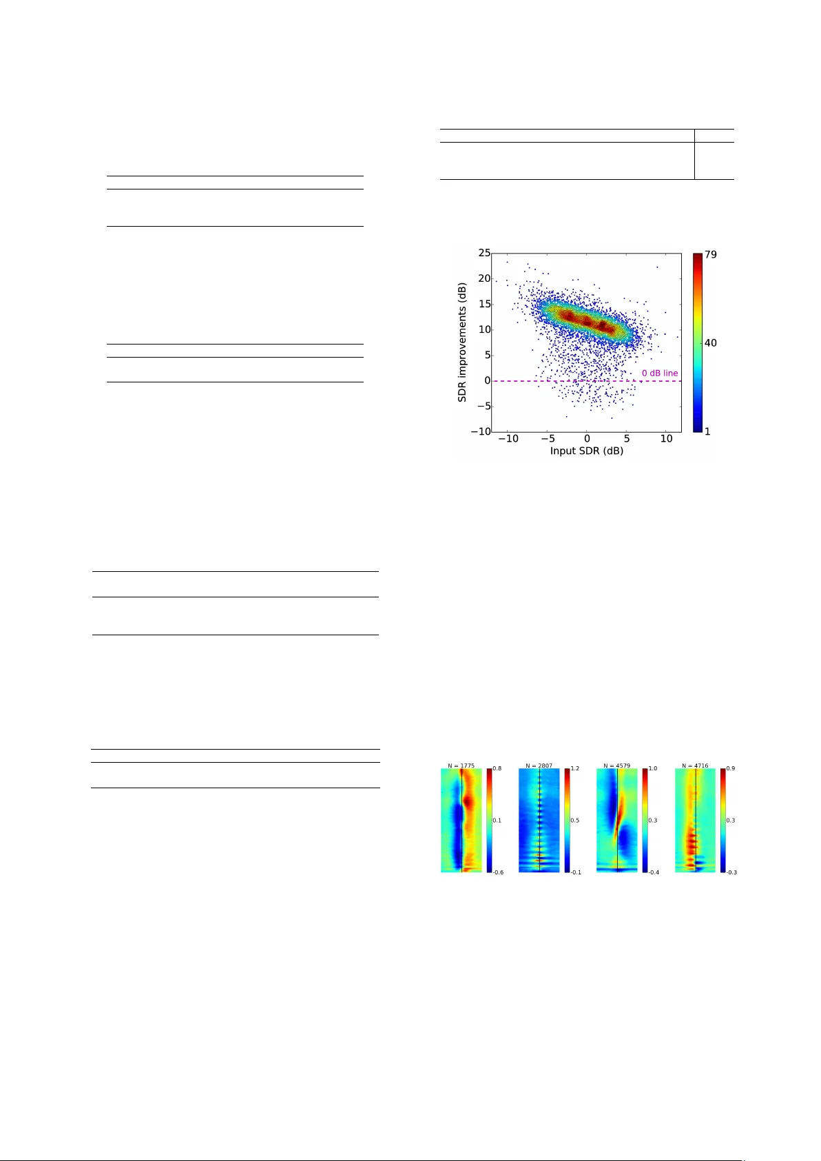
Single-Channel Multi-Speaker Separation using Deep Clustering Y usuf Isik 1 , 2 , 3 , J onathan Le Roux 1 , Zhuo Chen 1 , 4 , Shinji W atanabe 1 , J ohn R. Hershe y 1 1 Mitsubishi Electric Research Laboratories (MERL), Cambridge, MA, USA 2 Sabanci Uni versity , Istanbul, T urke y , 3 TUBIT AK BILGEM, K ocaeli, T urke y 4 Columbia Uni versity , New Y ork, NY , USA Abstract Deep clustering is a recently introduced deep learning architec- ture that uses discriminativ ely trained embeddings as the basis for clustering. It was recently applied to spectrogram segmen- tation, resulting in impressi ve results on speaker-independent multi-speaker separation. In this paper we extend the baseline system with an end-to-end signal approximation objective that greatly improv es performance on a challenging speech separa- tion. W e first significantly improve upon the baseline system performance by incorporating better regularization, larger tem- poral context, and a deeper architecture, culminating in an o ver - all improvement in signal to distortion ratio (SDR) of 10.3 dB compared to the baseline of 6.0 dB for two-speaker separation, as well as a 7.1 dB SDR improv ement for three-speak er separa- tion. W e then extend the model to incorporate an enhancement layer to refine the signal estimates, and perform end-to-end training through both the clustering and enhancement stages to maximize signal fidelity . W e ev aluate the results using auto- matic speech recognition. The new signal approximation ob- jectiv e, combined with end-to-end training, produces unprece- dented performance, reducing the word error rate (WER) from 89.1% down to 30.8%. This represents a major advancement tow ards solving the cocktail party problem. Index T erms : single-channel speech separation, embedding, deep learning 1. Introduction The human auditory system gives us the extraordinary abil- ity to con verse in the midst of a noisy throng of party goers. Solving this so-called coc ktail party problem [1] has proven extremely challenging for computers, and separating and rec- ognizing speech in such conditions has been the holy grail of speech processing for more than 50 years. Pre viously , no practi- cal method e xisted that could solv e the problem in general con- ditions, especially in the case of single channel speech mixtures. This w ork b uilds upon recent adv ances in single-channel sepa- ration, using a method known as deep clustering [2]. In deep clustering, a neural network is trained to assign an embed- ding vector to each element of a multi-dimensional signal, such that clustering the embeddings yields a desired segmentation of the signal. In the cocktail-party problem, the embeddings are assigned to each time-frequency (TF) index of the short- time Fourier transform (STFT) of the mixture of speech sig- nals. Clustering these embeddings yields an assignment of each TF bin to one of the inferred sources. These assignments are used as a masking function to extract the dominant parts of each source. Preliminary work on this method produced remarkable This work was done while Y . Isik was an intern at MERL. performance, improving SNR by 6 dB on the task of separating two unkno wn speakers from a single-channel mixture [2]. In this paper we present improvements and extensions that en- able a leap forward in separation quality , reaching le vels of im- prov ement that were previously out of reach (audio examples and scripts to generate the data used here are av ailable at [3]). In addition to improvements to the training procedure, we inv es- tigate the three speaker case, showing generalization between two- and three-speaker netw orks. The original deep clustering system was intended to only re- cov er a binary masks for each source, leaving recovery of the missing features to subsequent stages. In this paper , we incorpo- rate enhancement layers to refine the signal estimate. Using soft clustering, we can then train the entire system end-to-end , train- ing jointly through the deep clustering embeddings, the cluster - ing and enhancement stages. This allows us to directly use a sig- nal approximation objecti ve instead of the original mask-based deep clustering objectiv e. Prior work in this area includes auditory grouping approaches to computational auditory scene analysis (CASA) [4, 5]. These methods used hand-designed features to cluster the parts of the spectrum belonging to the same source. Their success was lim- ited by the lack of a machine learning framework. Such a frame- work was provided in subsequent work on spectral clustering [6], at the cost of prohibitiv e complexity . Generativ e models hav e also been proposed, beginning with [7]. In constrained tasks, super-human speech separation was first achiev ed using factorial HMMs [8, 9, 10, 11] and was extended to speaker -independent separation [12]. V ariants of non-negati ve matrix factorization [13, 14] and Bayesian non- parametric models [15, 16] hav e also been used. These methods suffer from computational complexity and difficulty of discrim- inativ e training. In contrast to the abo ve, deep learning approaches ha ve recently provided fast and accurate methods on simpler enhancement tasks [17, 18, 19, 20]. These methods treat the mask inferance as a classification problem, and hence can be discriminatively trained for accuracy without sacrificing speed. Howe ver they fail to learn in the speaker-independent case, where sources are of the same class [2], despite the work-around of choosing the best permutation of the network outputs during training. W e call this the permutation pr oblem : there are multiple valid out- put masks that dif fer only by a permutation of the order of the sources, so a global decision is needed to choose a permutation. Deep clustering solves the permutation problem by framing mask estimation as a clustering problem. T o do so, it produces an embedding for each time-frequency element in the spectro- gram, such that clustering the embeddings produces the desired segmentation. The representation is thus independent of per- mutation of the source labels. It can also flexibly represent any number of sources, allo wing the number of inferred sources to be decided at test time. Below we present the deep clustering model and further in vestigate its capabilities. W e then present extensions to allo w end-to-end training for signal fidelity . The results are ev aluated using an automatic speech recogni- tion model trained on clean speech. The end-to-end signal approximation produces unprecedented performance, reducing the word error rate (WER) from close to 89.1% WER do wn to 30.8% by using the end-to-end training. This represents a major advancement to wards solving the cocktail party problem. 2. Deep Clustering Model Here we revie w the deep clustering formalism presented in [2]. W e define as x a raw input signal and as X i = g i ( x ) , i ∈ { 1 , . . . , N } , a feature vector indexed by an element i . In audio signals, i is typically a TF index ( t, f ) , where t index es frame of the signal, f index es frequency , and X i = X t,f the value of the complex spectrogram at the corresponding TF bin. W e as- sume that the TF bins can be partitioned into sets of TF bins in which each source dominates. Once estimated, the partition for each source serves as a TF mask to be applied to X i , yielding the TF components of each source that are uncorrupted by other sources. The STFT can then be in verted to obtain estimates of each isolated source. The target partition in a giv en mixture is represented by the indicator Y = { y i,c } , mapping each element i to each of C components of the mixture, so that y i,c = 1 if element i is in cluster c . Then A = Y Y T is a binary affinity matrix that represents the cluster assignments in a permutation- independent way: A i,j = 1 if i and j belong to the same cluster and A i,j = 0 otherwise, and ( Y P )( Y P ) T = Y Y T for any permutation matrix P . T o estimate the partition, we seek D -dimensional embeddings V = f θ ( x ) ∈ R N × D , parameterized by θ , such that clustering the embeddings yields a partition of { 1 , . . . , N } that is close to the target. In [2] and this work, V = f θ ( X ) is based on a deep neural network that is a global function of the entire input signal X . Each embedding v i ∈ R D has unit norm, i.e., | v i | 2 = 1 . W e consider the embeddings V to implicitly represent an N × N estimated affinity matrix ˆ A = V V T , and we optimize the embeddings such that, for an input X , ˆ A matches the ideal affinities A . This is done by minimizing, with respect to V = f θ ( X ) , the training cost function C Y ( V ) = k ˆ A − A k 2 F = k V V T − Y Y T k 2 F (1) summed over training examples, where k · k 2 F is the squared Frobenius norm. Due to its low-rank nature, the objective and its gradient can be formulated so as to avoid operations on all pairs of elements, leading to an efficient implementation. At test time, the embeddings V = f θ ( X ) are computed on the test signal X , and the rows v i ∈ R D are clustered using K - means. The resulting cluster assignments ¯ Y are used as binary masks on the complex spectrogram of the mixture, to estimate the sources. 3. Impro vements to the T raining Recipe W e in vestigated sev eral approaches to improve performance ov er the baseline deep clustering method, including regulariza- tion such as drop-out, model size and shape, and training sched- ule. W e used the same feature extraction procedure as in [2], with log-magnitude STFT features as input, and we performed global mean-v ariance normalization as a pre-processing step. For all experiments we used we used rmsprop optimization [21] with a fix ed learning rate schedule, and early stopping based on cross-validation. Regularizing recurrent network units: Recurrent neural net- work (RNN) units, in particular LSTM structures, hav e been widely adopted in many tasks such as object detection, natural language processing, machine translation, and speech recogni- tion. Here we e xperiment with re gularizing them using dropout. LSTM nodes consist of a recurrent memory cell surrounded by gates controlling its input, output, and recurrent connections. The direct recurrent connections are element-wise and linear with weight 1, so that with the right setting of the gates, the memory is perpetuated, and otherwise more general recurrent processing is obtained. Dropout is a training regularization in which nodes are ran- domly set to zero. In recurrent network there is a concern that dropout could interfere with LSTM’s memorization ability; for example, [22] used it only on feed-forw ard connections, but not on the recurrent ones. Recurr ent dropout samples the set of dropout nodes once for each sequence, and applies dropout to the same nodes at ev ery time step for that sequence. Applying recurrent dropout to the LSTM memory cells recently yielded performance improvements on phoneme and speech recognition tasks with BLSTM acoustic models [23]. In this work, we sampled the dropout masks once at each time step for the forward connections, and only once for each se- quence for the recurrent connections. W e used the same recur - rent dropout mask for each gate. Architectur e: W e investig ated using deeper and wider archi- tectures. The neural network model used in [2] was a two layer bidirectional long short-term memory (BLSTM) network fol- lowed by a feed-forward layer to produce embeddings. W e show that expanding the network size improv es performance for our task. T emporal context: During training, the utterances are divided into fixed length non-overlapping segments, and gradients are computed using shuf fled mini-batches of these segments, as in [2]. Shorter segments increase the di versity within each batch, and may make an easier starting point for training, since the speech does not change as much ov er the se gment. Howe ver , at test time, the network and clustering are giv en the entire utter - ance, so that the permutation problem can be solved globally . So we may also expect that training on longer segments would improv e performance in the end. In experiments below , we inv estigate training segment lengths of 100 versus 400, and show that although the longer seg- ments work better, pretraining with shorter segments followed by training with longer segments leads to better performance on this task. This is an example of curriculum learning [24], in which starting with an easier task improv es learning and gener - alization. Multi-speaker training: Pre vious experiments [2] sho wed pre- liminary results on generalization from two speaker training to a three-speaker separation task. Here we further in vestigate generalization from three-speaker training to two-speaker sep- aration, as well as multi-style training on both two and three- speaker mixtures, and show that the multi-style training can achiev e the best performance on both tasks. 4. Optimizing Signal Reconstruction Deep clustering solves the dif ficult problem of segmenting the spectrogram into re gions dominated by each source. It does not howe ver solve the problem of recov ering the sources in regions strongly dominated by other sources. Giv en the segmentation, this is ar guably an easier problem. W e propose to use a second- stage enhancement network to obtain better source estimates, in particular for the missing regions. For each source c , the enhancement network first processes the concatenation of the amplitude spectrogram x of the mixture and that ˆ s c of the deep clustering estimate through a BLSTM layer and a feed-forward linear layer , to produce an output z c . Sequence-le vel mean and variance normalization is applied to the input, and the net- work parameters are shared for all sources. A soft-max is then used to combine the outputs z c across sources, forming a mask m c,i = e z c,i / P c 0 e z c 0 ,i at each TF bin i . This mask is ap- plied to the mixture, yielding the final estimate ˜ s c,i = m c,i x i . During training, we optimize the enhancement cost function C E = min π ∈P P c,i ( s c,i − ˜ s π ( c ) ,i ) 2 , where P is the set of permutations on { 1 , . . . , C } . Since the enhancement network is trained to directly improv e the signal reconstruction, it may improv e upon deep clustering, especially in regions where the signal is dominated by other sources. 5. End-to-End T raining In order to consider end-to-end training in the sense of jointly training the deep clustering with the enhancement stage, we need to compute gradients of the clustering step. In [2], hard K -means clustering was used to cluster the embeddings. The resulting binary masks cannot be directly optimized to improv e signal fidelity , because the optimal masks are generally contin- uous, and because the hard clustering is not differentiable. Here we propose a soft K -means algorithm that enables us to directly optimize the estimated speech for signal fidelity . In [2], clustering was performed with equal weights on the TF embeddings, although weights were used in the training objec- tiv e in order to train only on TF elements with significant en- ergy . Here we introduce similar weights weights w i for each embedding v i to focus the clustering on TF elements with sig- nificant energy . The goal is mainly to avoid clustering silence regions, which may have noisy embeddings, and for which mask estimation errors are inconsequential. The soft weighted K -means algorithm can be interpreted as a weighted expectation maximization (EM) algorithm for a Gaus- sian mixture model with tied circular covariances. It alternates between computing the assignment of e very embe dding to each centroid, and updating the centroids: γ i,c = e − α | v i − µ c | 2 P c 0 e − α | v i − µ c 0 | 2 , µ c = P i γ i,c w i v i P i γ i,c w i , (2) where µ c is the estimated mean of cluster c , and γ i,j is the esti- mated assignment of embedding i to the cluster c . The parame- ter α controls the hardness of the clustering. As the value of α increases, the algorithm approaches K -means. The weights w i may be set in a variety of ways. A reasonable choice could be to set w i according to the po wer of the mixture in each TF bin. Here we set the weights to 1 , except in silence TF bins where the weight is set to 0 . Silence is defined using a threshold on the energy relative to the maximum of the mixture. End-to-end training is performed by unfolding the steps of (2), and treating them as layers in a clustering network, according to the general framework known as deep unfolding [25]. The gradients of each step are thus passed to the previous layers using standard back-propagation. 6. Experiments Experimental setup: W e ev aluate deep clustering on a single- channel speaker-independent speech separation task, consider- ing mixtures of two and three speakers with all gender combi- nations. For two-speaker experiments, we use the corpus in- troduced in [2], derived from the W all Street Journal (WSJ0) corpus. It consists in a 30 h training set and a 10 h v alida- tion set with two-speaker mixtures generated by randomly se- lecting utterances by different speak ers from the WSJ0 training set si_tr_s , and mixing them at various signal-to-noise ratios (SNR) randomly chosen between 0 dB and 10 dB. The vali- dation set was here used to optimize some tuning parameters. The 5 h test set consists in mixtures similarly generated using utterances from 16 speakers from the WSJ0 development set si_dt_05 and ev aluation set si_et_05 . The speakers are dif- ferent from those in our training and validation sets, leading to a speaker -independent separation task. For three-speaker experi- ments, we created a corpus similar to the two-speak er one, with the same amounts of data generated from the same datasets. All data were downsampled to 8 kHz before processing to reduce computational and memory costs. The input features X were the log spectral magnitudes of the speech mixture, computed using a short-time Fourier transform (STFT) with a 32 ms sine window and 8 ms shift. The scores are reported in terms of signal-to-distortion ratio (SDR), which we define as scale-inv ariant SNR. As oracle up- per bounds on performance for our datasets, we report in T able 1 the results obtained using two types of “ideal” masks: the ideal binary mask (ibm) defined as a ibm i = δ ( | s i | > max j 6 = i | s j | ) , which leads to highest SNR among all binary masks, and a “W iener-lik e” filter (wf) defined as a wf i = | s i | 2 / P j | s j | 2 , which empirically leads to good SNR, with v alues in [0 , 1] [26, 27]. Here s i denotes the time-frequenc y representation of speaker i . CASA [5] and previous deep clustering [2] results are also shown for the tw o-speaker set. T able 1: SDR (dB) improvements using the ideal binary mask (ibm), oracle W iener-lik e filter (wf), compared to prior methods dpcl [2] and CASA [5] on the two- and three-speaker test sets. # speakers ibm wf dpcl v1 [2] CASA [5] 2 13.5 13.9 6.0 3.1 3 13.3 13.8 - - The initial system, based on [2], trains a deep clustering model on 100-frame segments from the two-speaker mixtures. The network, with 2 BLSTM layers, each having 300 forward and 300 backward LSTM cells, is denoted as 300 × 2 . The learn- ing rate for the rmsprop algorithm [21] was λ = 0 . 001 × (1 / 2) b / 50 c , where  is the epoch number . Regularization: W e first considered improving performance of the baseline using common regularization practices. T able 2 shows the contribution of dropout ( p = 0 . 5 ) on feed-forward connections, recurrent dropout ( p = 0 . 2 ), and gradient normal- ization ( |∇| ≤ 200 ), where the parameters were tuned on de- velopment data. T ogether these result in a 3.3 dB improvement in SDR relativ e to the baseline. T able 2: Decomposition of the SDR improvements (dB) on the two-speaker test set using 300 × 2 model. rmsprop +dropout +recurrent dropout +norm constraint 5.7 8.0 8.9 9.0 Architectur e: V arious network architectures were inv estigated by increasing the number of hidden units and number of BLSTM layers, as shown in T able 3. An improvement of 9.4 dB SDR was obtained with a deeper 300 × 4 architecture, with 4 BLSTM layers and 300 units in each LSTM. T able 3: SDR (dB) improvements on the two-speaker test set for different architecture sizes. model same-gender different-gender o verall 300 × 2 6.4 11.2 9.0 600 × 2 6.1 11.5 9.0 300 × 4 7.1 11.5 9.4 Pre-training of temporal context: Training the model with segments of 400 frames, after pre-training using 100-frame seg- ments, boosts performance to 10.3 dB, as shown in T able 4, from 9 . 9 dB without pre-training. Results for the remaining ex- periments are based on the pre-trained 300 × 4 model. T able 4: SDR (dB) improvements on the two-speaker test set after training with 400 frame length segments. model same-gender different-gender o verall 600 × 2 7.8 11.7 9.9 300 × 4 8.6 11.7 10.3 Multi-speaker training: W e train the model further with a blend of two- and three-speaker mixtures. For comparison, we also trained a model using only three-speaker mixtures, again training first ov er 100-frame se gments, then over 400-frame segments. The performance of the models trained on two- speaker mixtures only , on three-speaker mixtures only , and us- ing the multi-speaker training, are shown in T able 5. The three- speaker mixture model seems to generalize better to two speak- ers than vice versa, whereas the multi-speaker trained model performed the best on both tasks. T able 5: Generalization across dif ferent numbers of speak ers in terms of SDR improv ements (dB). T raining data T est data 2 speaker 3 speaker 2 speaker 10.3 2.1 3 speaker 8.5 7.1 Mixed curriculum 10.5 7.1 Soft clustering: The choice of the clustering hardness parame- ter α and the weights on TF bins is analyzed on the validation set, with results in T able 6. The use of weights to ignore silence improv es performance with diminishing returns for larg α . The best result is for α = 5 . T able 6: Performance as a function of soft weighted K -means parameters on the two-speaker v alidation set. weights α = 2 α = 5 α = 10 hard K -means all equal 5.0 10.1 10.1 10.3 mask silent 9.1 10.3 10.2 10.3 End-to-end training: Finally , we inv estigate end-to-end train- ing, using a second-stage enhancement network on top of the deep clustering (‘dpcl’) model. Our enhancement network fea- tures two BLSTM layers with 300 units in each LSTM layer, with one instance per source followed by a soft-max layer to form a masking function. W e first trained the enhancement net- work separately (‘dpcl + enh’), follo wed by end-to-end fine- tuning in combination with the dpcl model (‘end-to-end’). T a- ble 7 shows the improv ement in SDR as well as magnitude SNR (SNR computed on the magnitude spectrograms). The magnitude SNR is insensiti ve to phase estimation errors in- troduced by using the noisy phases for reconstruction, whereas the SDR might get worse as a result of phase errors, even if the amplitudes are accurate. Speech recognition uses features based on the amplitudes, and hence the improv ements in mag- nitude SNR seem to predict the improv ements in WER due to T able 7: SDR / Magnitude SNR improvements (dB) and WER with enhancement network. model same-gender different-gender ov erall WER dpcl 8.6 / 8.9 11.7 / 11.4 10.3 / 10.2 87.9 % dpcl + enh 9.1 / 10.7 11.9 / 13.6 10.6 / 12.3 32.8 % end-to-end 9.4 / 11.1 12.0 / 13.7 10.8 / 12.5 30.8% the enhancement and end-to-end training. Fig. 1 shows that the SDR improv ements of the end-to-end model are consistently good on nearly all of the two-speaker test mixtures. Figure 1: Scatter plot for the input SDRs and the corresponding improv ements. Color indicates density . ASR performance: W e ev aluated ASR performance (WER) with GMM-based clean-speech WSJ models obtained by a stan- dard Kaldi recipe [28]. The noisy baseline result on the mix- tures is 89.1 %, while the result on the clean speech is 19.9 %. The raw output from dpcl did not work well, despite good per- ceptual quality , possibly due to the ef fect of near-zero values in the masked spectrum, which is known to degrade ASR per- formance. Howev er , the enhancement networks significantly mitigated the degradation, and finally obtained 30.8 % with the end-to-end network. V isualization: T o gain insight into network functioning, we performed rev erse correlation experiments. For each node, we average the 50-frame patches of input centered at the time when the node is active (e.g., the node is at 80% of its max- imum value). Fig. 2 shows a variety of interesting patterns, which seem to reflect such properties as onsets, pitch, frequency chirps, and vo wel-fricative transitions. (a) onset (b) pitch (c) chirp (d) transition Figure 2: Example spike-triggered spectrogram av erages with 50-frame context, for active LSTM nodes in the second layer . N is the number of active frames for the corresponding node. Conclusion: W e have improved and extended the deep clus- tering framework to perform end-to-end training for signal re- construction quality for the first time. W e show significant im- prov ements to performance both on signal quality metrics and speech recognition error rates. 7. References [1] A. S. Bregman, Auditory scene analysis: The per ceptual or ganization of sound . MIT press, 1990. [2] J. R. Hershey , Z. Chen, J. Le Roux, and S. W atanabe, “Deep clustering: Discriminati ve embeddings for seg- mentation and separation, ” in Pr oc. ICASSP , Mar . 2016. [3] Y . Isik, J. Le Roux, Z. Chen, S. W atanabe, and J. R. Hershey , “Deep clustering: Audio examples, ” http://www . merl.com/demos/deep- clustering, 2016, [Online]. [4] M. P . Cooke, “Modelling auditory processing and organi- sation, ” Ph.D. dissertation, Univ . of Shef field, 1991. [5] K. Hu and D. W ang, “ An unsupervised approach to cochannel speech separation, ” IEEE T ransactions on A u- dio, Speech, and Language Processing , vol. 21, no. 1, pp. 122–131, 2013. [6] F . R. Bach and M. I. Jordan, “Learning spectral clustering, with application to speech separation, ” JMLR , vol. 7, pp. 1963–2001, 2006. [7] D. P . W . Ellis, “Prediction-driven computational auditory scene analysis, ” Ph.D. dissertation, MIT , 1996. [8] J. R. Hershey , S. J. Rennie, P . A. Olsen, and T . T . Krist- jansson, “Super-human multi-talker speech recognition: A graphical modeling approach, ” Comput. Speech Lang. , vol. 24, no. 1, pp. 45–66, 2010. [9] S. J. Rennie, J. R. Hershey , and P . A. Olsen, “Single- channel multitalker speech recognition, ” IEEE Signal Pro- cess. Mag . , vol. 27, no. 6, pp. 66–80, 2010. [10] M. Cooke, J. R. Hershey , and S. J. Rennie, “Monaural speech separation and recognition challenge, ” Comput. Speech Lang. , vol. 24, no. 1, pp. 1–15, 2010. [11] T . V irtanen, “Speech recognition using factorial hidden Markov models for separation in the feature space, ” in Pr oc. Interspeech , 2006. [12] R. J. W eiss, “Underdetermined source separation using speaker subspace models, ” Ph.D. dissertation, Columbia Univ ersity , 2009. [13] P . Smaragdis, “Conv olutiv e speech bases and their appli- cation to supervised speech separation, ” IEEE T rans. Au- dio, Speech, Language Pr ocess. , vol. 15, no. 1, pp. 1–12, 2007. [14] U. Simsekli, J. Le Roux, and J. Hershey , “Non-negati ve source-filter dynamical system for speech enhancement, ” in Pr oc. ICASSP , Florence, Italy , May 2014. [15] D. M. Blei, P . R. Cook, and M. Hoffman, “Bayesian non- parametric matrix factorization for recorded music, ” in Pr oc. ICML , 2010, pp. 439–446. [16] M. Nakano, J. Le Roux, H. Kameoka, T . Nakamura, N. Ono, and S. Sagayama, “Bayesian nonparametric spec- trogram modeling based on infinite factorial infinite hid- den markov model, ” in Pr oc. W ASP AA , 2011, pp. 325– 328. [17] F . W eninger , H. Erdogan, S. W atanabe, E. V incent, J. Le Roux, J. R. Hershey , and B. Schuller, “Speech en- hancement with LSTM recurrent neural networks and its application to noise-robust ASR, ” in Latent V ariable Anal- ysis and Signal Separation . Springer , 2015, pp. 91–99. [18] Y . W ang, A. Narayanan, and D. W ang, “On training tar- gets for supervised speech separation, ” IEEE/ACM T rans. Audio, Speech, and Language Pr ocess. , vol. 22, no. 12, pp. 1849–1858, 2014. [19] Y . Xu, J. Du, L.-R. Dai, and C.-H. Lee, “ An experimental study on speech enhancement based on deep neural net- works, ” IEEE Signal Pr ocessing Letters , vol. 21, no. 1, pp. 65–68, 2014. [20] P .-S. Huang, M. Kim, M. Hasega wa-Johnson, and P . Smaragdis, “Joint optimization of masks and deep re- current neural networks for monaural source separation, ” arXiv pr eprint arXiv:1502.04149 , 2015. [21] T . Tieleman and G. Hinton, “Lecture 6.5—RmsProp: Di- vide the gradient by a running a verage of its recent magni- tude, ” COURSERA: Neural Networks for Machine Learn- ing, 2012. [22] W . Zaremba, I. Sutskev er , and O. V inyals, “Re- current neural network regularization, ” arXiv preprint arXiv:1409.2329 , 2014. [23] T . Moon, H. Choi, H. Lee, and I. Song, “RnnDrop: A nov el dropout for RNNs in ASR, ” Pr oc. ASRU , 2015. [24] Y . Bengio, J. Louradour , R. Collobert, and J. W eston, “Curriculum learning, ” in Pr oc. ICML , 2009, pp. 41–48. [25] J. R. Hershey , J. Le Roux, and F . W eninger , “Deep unfolding: Model-based inspiration of novel deep architectures, ” arXiv preprint , Sep. 2014. [Online]. A v ailable: http://arxiv .org/abs/1409.2574 [26] D. W ang, “On ideal binary mask as the computational goal of auditory scene analysis, ” in Speech separation by hu- mans and machines . Springer , 2005, pp. 181–197. [27] H. Erdogan, J. R. Hershey , S. W atanabe, and J. Le Roux, “Phase-sensitiv e and recognition-boosted speech sepa- ration using deep recurrent neural networks, ” in Pr oc. ICASSP , Apr . 2015. [28] D. Pov ey , A. Ghoshal, G. Boulianne, L. Bur get, O. Glem- bek, N. Goel, M. Hannemann, P . Motlicek, Y . Qian, P . Schwarz et al. , “The Kaldi speech recognition toolkit, ” in Pr oc. ASRU , 2011.