Efficient Reinforcement Learning in Deterministic Systems with Value Function Generalization

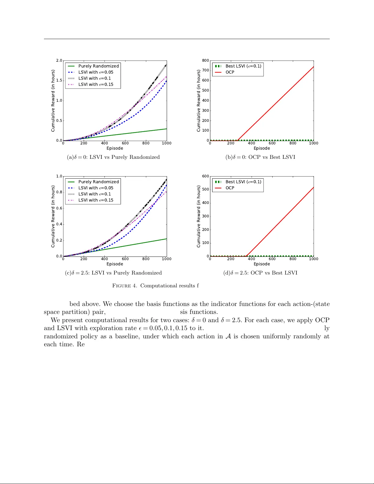
Eﬃcien t Reinforcemen t Learning in Deterministic Systems with V alue F unction Generalization Zheng W en Adobe Research, zwen@adobe.com , Benjamin V an Ro y Stanford University , bvr@stanford.edu , W e consider the problem of reinforcemen t learning o ver episodes of a ﬁnite-horizon deterministic system and as a solution propose optimistic c onstr aint pr op agation (OCP) , an algorithm designed to syn thesize eﬃcien t exploration and v alue function generalization. W e establish that when the true v alue function Q ∗ lies within a known h yp othesis class Q , OCP selects optimal actions o ver all but at most dim E [ Q ] episo des, where dim E denotes the eluder dimension . W e establish further eﬃciency and asymptotic p erformance guaran tees that apply ev en if Q ∗ do es not lie in Q , for the special case where Q is the span of pre-speciﬁed indicator functions o ver disjoint sets. W e also discuss the computational complexit y of OCP and presen t computational results in volving t wo illustrativ e examples. Key wor ds : Reinforcemen t Learning, Eﬃcient Exploration, V alue F unction Generalization, Appro ximate Dynamic Programming 1. In tro duction A gro wing b ody of work on eﬃcien t reinforcement learning pro vides algo- rithms with guaran tees on sample and computational eﬃciency (see, e.g., [ 13 , 6 , 2 , 30 , 4 , 9 ] and references therein). This literature highligh ts the p oin t that an eﬀective exploration sc heme is critical to the design of any eﬃcien t reinforcemen t learning algorithm. In particular, popular explo- ration sc hemes such as  -greedy , Boltzmann, and kno wledge gradient (see [ 27 ]) can require learning times that gro w exp onen tially in the num b er of states and/or the planning horizon (see [ 38 , 29 ]). The aforementioned literature fo cusses on tabula r asa learning; that is, algorithms aim to learn with little or no prior kno wledge ab out transition probabilities and rewards. Suc h algorithms require learning times that gro w at least linearly with the n um b er of states. Despite the v aluable insigh ts that ha ve b een generated through their design and analysis, these algorithms are of limited practical imp ort because state spaces in most con texts of practical interest are enormous. There is a need for algorithms that generalize from past exp erience in order to learn how to make eﬀective decisions in reasonable time. There has b een m uch w ork on reinforcement learning algorithms that generalize (see, e.g., [ 5 , 31 , 32 , 24 ] and references therein). Most of these algorithms do not come with statistical or computational eﬃciency guarantees, though there are a few notew orthy exceptions, which we no w discuss. A num b er of results treat p olicy-based algorithms (see [ 10 , 3 ] and references therein), in whic h the goal is to select high-p erformers among a pre-sp eciﬁed collection of p olicies as learning progresses. Though in teresting results hav e b een pro duced in this line of work, each entails quite restrictiv e assumptions or do es not mak e strong guaran tees. Another b ody of work fo cuses on mo del-based algorithms. An algorithm prop osed by Kearns and Koller [ 12 ] ﬁts a factored mo del to observed data and mak es decisions based on the ﬁtted mo del. The authors establish a sample complexit y bound that is polynomial in the n um b er of mo del parameters rather than the num b er of states, but the algorithm is computationally in tractable b ecause of the diﬃcult y of solving factored 1 W en and V an Ro y: Eﬃcient R einfor c ement L e arning in Deterministic Systems 2 MDPs. Lattimore et al. [ 15 ] prop ose a no vel algorithm for the case where the true en vironment is kno wn to b elong to a ﬁnite or compact class of mo dels, and shows that its sample complexity is p olynomial in the cardinality of the mo del class if the model class is ﬁnite, or the  -cov ering-num b er if the mo del class is compact. Though this result is theoretically interesting, for most mo del classes of interest, the  -cov ering-num b er is enormous since it t ypically grows exp onen tially in the n umber of free parameters. Ortner and Ryabk o [ 20 ] establish a regret b ound for an algorithm that applies to problems with con tinuous state spaces and H¨ older-con tin uous rewards and transition k ernels. Though the results represen t an in teresting con tribution to the literature, a couple of features of the regret b ound weak en its practical implications. First, regret gro ws linearly with the H¨ older constan t of the transition kernel, which for most con texts of practical relev ance grows exp onen tially in the n um b er of state v ariables. Second, the dep endence on time b ecomes arbitrarily close to linear as the dimension of the state space grows. P azis and Parr [ 22 ] also consider problems with contin uous state spaces. They assume that the Q-functions are Lipschitz-con tinuous or H¨ older-con tin uous and establish a sample complexit y bound. Though the results are interesting and signiﬁcan t, the sample complexit y b ound is log-linear in the co vering num b er of the state-action space, whic h also typically gro ws exp onen tially in the num b er of free parameters for most practical problems. Reinforcement learning in linear systems with quadratic cost is treated in Abbasi-Y adkori and Szep esv´ ari [ 1 ]. The metho d prop osed is sho wn to realize regret that grows with the square ro ot of time. The result is interesting and the prop ert y is desirable, but to the b est of our knowledge, expressions derived for regret in the analysis exhibit an exp onen tial dep endence on the num b er of state v ariables, and further, w e are not aw are of a computationally eﬃcient w a y of implementing the proposed metho d. This w ork w as extended b y Ibrahimi et al. [ 8 ] to address linear systems with sparse structure. Here, there are eﬃciency guarantees that scale gracefully with the num b er of state v ariables, but only under sparsit y and other tec hnical assumptions. The most p opular approac h to generalization in the applied reinforcemen t learning literature in v olv es ﬁtting parameterized v alue functions. Suc h approac hes relate closely to supervised learning in that they learn functions from state-action pairs to v alue, though a diﬀerence is that v alue is inﬂuenced by action and observed only through dela yed feedback. One adv an tage ov er model learning approaches is that, given a ﬁtted v alue function, decisions can b e made without solving an often intractable control problem. W e see this as a promising direction, though there currently is a lack of theoretical results that provide attractive b ounds on learning time with v alue function generalization. A relev an t pap er along these lines is [ 16 ], which studies eﬃcient reinforcemen t learning with v alue function generalization in the KWIK framework (see [ 17 ]) and reduces the problem to eﬃcient KWIK online regression. How ever, the authors do not show how to solv e the general KWIK online regression problem eﬃcien tly , and it is not even clear whether this is possible. Th us, though the result of Li and Littman [ 16 ] is in teresting, it do es not provide a pro v ably eﬃcien t algorithm for general reinforcemen t learning problems. How ever, it is w orth mentioning that Li et al. [ 17 ] has provided a solution to KWIK online regression with deterministic linear functions. As w e will discuss later, this can b e seen as a special case of the coherent learning problems w e consider in Section 5.2 . An imp ortan t challenge that remains is to couple exploration and v alue function generalization in a pro v ably eﬀective w ay , and in particular, to establish sample and computational eﬃciency guaran tees that scale gracefully with the planning horizon and mo del complexit y . In this pap er, we aim to make progress in this direction. T o start with a simple context, we restrict our atten tion to deterministic systems that evolv e o v er ﬁnite time horizons, and we consider episo dic learning, in whic h an agen t rep eatedly interacts with the same system. As a solution to the problem, w e pro- p ose optimistic c onstr aint pr op agation (OCP) , a computationally eﬃcien t reinforcement learning algorithm designed to synthesize eﬃcient exploration and v alue function generalization. W e estab- lish that when the true v alue function Q ∗ lies within the h yp othesis class Q , OCP selects optimal W en and V an Ro y: Eﬃcient R einfor c ement L e arning in Deterministic Systems 3 actions o ver all but at most dim E [ Q ] episodes. Here, dim E denotes the eluder dimension , which quan tiﬁes complexit y of the h yp othesis class. A corollary of this result is that regret is b ounded b y a function that is constan t o v er time and linear in the problem horizon and eluder dimension. T o put our aforemen tioned result in p ersp ectiv e, it is useful to relate it to other lines of work. Consider ﬁrst the broad area of reinforcemen t learning algorithms that ﬁt v alue functions, such as SARSA [ 25 ]. Ev en with the most commonly used sort of h yp othesis class Q , which is made up of linear com binations of ﬁxed basis functions, and even when the hypothesis class contains the true v alue function Q ∗ , there are no guarantees that these algorithms will eﬃciently learn to mak e near-optimal decisions. On the other hand, our result implies that OCP attains near-optimal p erformance in time th at scales linearly with the n umber of basis functions. No w consider the more sp ecialized con text of a deterministic linear system with quadratic cost and a ﬁnite time horizon. The analysis of Abbasi-Y adk ori and Szep esv´ ari [ 1 ] can b e leveraged to pro duce regret b ounds that scale exp onen tially in the num b er of state v ariables. On the other hand, using a hypothesis space Q consisting of quadratic functions of state-action pairs, the results of this pap er sho w that OCP b eha ves near optimally within time that scale s quadratically in the n umber of state and action v ariables. W e also establish eﬃciency and asymptotic p erformance guarantees that apply to agnostic rein- forcemen t learning, where Q ∗ do es not necessarily lie in Q . In particular, w e consider the case where Q is the span of pre-sp eciﬁed indicator functions o v er disjoin t sets. Our results here add to the literature on agnostic reinforcement learning with suc h a h yp othesis class [ 28 , 33 , 7 , 34 ]. Prior work in this area has pro duced interesting algorithms and insights, as well as b ounds on p erformance loss asso ciated with p oten tial limits of conv ergence, but no con vergence or eﬃciency guaran tees. These results build on and add to those rep orted in an earlier pap er that we published in pro ceedings of a conference [ 37 ]. In addition to establishing theoretical results, we present computational results inv olving t w o illustrativ e examples: a synthetic deterministic Marko v chain and the inv erted p endulum control problem considered in Lagoudakis et al. [ 14 ]. W e compare OCP against least-squares v alue iteration (LSVI), a classical reinforcemen t learning algorithm. In b oth exp eriments, the p erformance of OCP is orders of magnitude b etter than that of LSVI. It is worth mentioning that in the inv erted p endulum example, w e consider a case in which there are small sto c hastic disturbances additiv e to the con trol. This result sho ws that, though OCP is designed for deterministic systems, it might also w ork w ell in sto c hastic en vironmen ts, esp ecially when the magnitude of the sto c hastic disturbances is small. Finally , it is w orth pointing out that reinforcement learning algorithms are often used to appro xi- mate solutions to large-scale dynamic programs, where the system mo dels are known . By known , w e mean that, given suﬃcient compute p ow er, one can determine the exp ected single-p erio d rewards and transition probabilities with any desired level of accuracy in the absence of an y additional empirical data. In such con texts, there is no need for statistical learning as c hallenges are purely computational. Nev ertheless, reinforcement learning algorithms make up p opular solution tec h- niques for such problems, and our algorithm and results also serve as con tributions to the ﬁeld of appro ximate dynamic programming. Speciﬁcally , prior appro ximate dynamic programming algo- rithms that ﬁt a linear com bination of basis functions to the v alue function, even when the optimal v alue function is within the span, come with no guarantees that a near-optimal p olicy can b e computed eﬃcien tly . In this pap er, we establish such a guarantee for OCP . 2. Episo dic Reinforcement Learning i n Deterministic Systems W e consider a class of reinforcemen t learning problems in whic h an agent rep eatedly interacts with an unknown discrete- time deterministic ﬁnite-horizon Mark ov decision process (MDP). Each interaction is referred to as an episo de , and the agent’s ob jective is to maximize the exp ected cumulativ e reward o ver episo des. W en and V an Ro y: Eﬃcient R einfor c ement L e arning in Deterministic Systems 4 The system is iden tiﬁed b y a sextuple M = ( S , A , H , F, R , S ) , where S is the state space, A is the action space, H is the horizon, F is a system function, R is a rew ard function and S is a sequence of states. If action a ∈ A is selected while the system is in state x ∈ S at p erio d t = 0 , 1 , · · · , H − 1, a reward of R t ( x, a ) is realized; furthermore, if t < H − 1, the state transitions to F t ( x, a ). Each episo de terminates at p eriod H − 1, and then a new episo de b egins. The initial state of episo de j is the j th element of S . T o represent the history of actions and observ ations ov er multiple episo des, w e will often index v ariables b y b oth episo de and p erio d. F or example, x j,t and a j,t denote the state and action at p eriod t of episo de j , where j = 0 , 1 , · · · and t = 0 , 1 , · · · , H − 1. T o count the total num b er of steps since the agen t started learning, w e sa y p eriod t in episo de j is time j H + t . A (deterministic) p olicy µ = ( µ 0 , . . . , µ H − 1 ) is a sequence of functions, each mapping S to A . F or eac h p olicy µ , deﬁne a v alue function V µ t ( x ) = P H − 1 τ = t R τ ( x τ , a τ ), where x t = x , x τ +1 = F τ ( x τ , a τ ), and a τ = µ τ ( x τ ). The optimal v alue function is deﬁned by V ∗ t ( x ) = sup µ V µ t ( x ). A p olicy µ ∗ is said to b e optimal if V µ ∗ = V ∗ . Throughout this pap er, we will restrict attention to systems M = ( S , A , H , F, R , S ) that admit optimal p olicies. Note that this restriction incurs no loss of generality when the action space is ﬁnite. It is also useful to deﬁne an action-con tingen t optimal v alue function: Q ∗ t ( x, a ) = R t ( x, a ) + V ∗ t +1 ( F t ( x, a )) for t < H − 1, and Q ∗ H − 1 ( x, a ) = R H − 1 ( x, a ). Then, a p olicy µ ∗ is optimal if µ ∗ t ( x ) ∈ arg max a ∈A Q ∗ t ( x, a ) for all ( x, t ). This pap er considers a reinforcement learning framework in which the agen t initially knows the state space S , the action space A , the horizon H , and p ossibly some prior information ab out the v alue function, but do es not kno w an ything else ab out the system function F , the rew ard function R , or the sequence of the initial states S . A reinforcement learning algorithm generates each action a j,t based on observ ations made up to the t th p eriod of the j th episo de, including all states, actions, and rewards observed in previous episo des and earlier in the curren t episo de, as well as S , A , H , and p ossible prior information. In eac h episode, the algorithm realizes reward R ( j ) = P H − 1 t =0 R t ( x j,t , a j,t ) . Note that R ( j ) ≤ V ∗ 0 ( x j, 0 ) for eac h j th episode. T o quan tify the p erformance of a reinforcemen t learning algorithm, for any  ≥ 0, we deﬁne the  -sub optimal sample c omplexity of that algorithm as the num b er of episo des J L for which R ( j ) < V ∗ 0 ( x j, 0 ) −  . Moreov er, w e say a reinforcemen t learning algorithm is sample eﬃcien t in a giv en setting if for some reasonable c hoice of  , the worst-case  -sub optimal sample complexity of that algorithm is small for that setting. Note that if the reward function R is b ounded, with | R t ( x, a ) | ≤ R for all ( x, a, t ), then a b ound on  -sub optimal sample complexit y J L also implies a b ound on regret ov er episo des exp erienced prior to time T , deﬁned b y Regret( T ) = P b T /H c− 1 j =0 ( V ∗ 0 ( x j, 0 ) − R ( j ) ). In particular, Regret( T ) ≤ 2 RH J L +  b T /H c . 3. Ineﬃcien t Exploration Sc hemes Before pro ceeding, it is worth p oin ting out that for the reinforcemen t learning problem prop osed ab o ve, a n um b er of p opular exploration sc hemes give rise to exp onen tially large regret. Even in the tabula r asa case, Boltzmann 1 and  -greedy exploration sc hemes (see, e.g., [ 23 ]), for example, lead to worst-case regret exp onen tial in H and/or |S | . Also, the kno wledge gradient exploration sc heme (see, e.g., [ 24 ] and [ 27 ]) can conv erge to sub optimal p olicies, and even when the ultimate p olicy is optimal, regret can grow exp onen tially in H and/or |S | . Th us, ev en for the tabula r asa case, eﬃcient exploration sc hemes are necessary for an algorithm to ac hiev e regret p olynomial in H and |S | . T o illustrate how simple exploration schemes give rise to exp onentially large regret and how OCP will mitigate that, consider the follo wing simple example. 1 Notice that in this pap er, w e assume that the state transition mo del of the deterministic system is unknown. Some literature (see [ 18 ] and references therein) consider settings in which the state transition mo del is known but the rew ard function is unknown, and establish that exploration sc hemes similar to Boltzmann exploration achiev e regret p olynomial in H (or, more generally , a notion of mixing time) and |S | . W en and V an Ro y: Eﬃcient R einfor c ement L e arning in Deterministic Systems 5 x=0$ x=1$ x=2$ x=3$ x=N)2$ x=N)1$ Figure 1. Deterministic system for whic h Boltzmann and  -greedy exploration are ineﬃcient. Example 1. Consider the deterministic system illustrated in Figure 1 . Eac h no de repre- sen ts a state, and each arrow corresp onds to a p ossible state transition. The state space is S = { 0 , 1 , · · · , N − 1 } and the action space is A =  a (1) , a (2)  . If the agent tak es action a (1) at state x = 0 , 1 , · · · , N − 2, the state transitions to y = [ x − 1] + . On the other hand, if the agent takes action a (2) at state x = 0 , 1 , · · · , N − 2, the state transitions to y = x + 1. State N − 1 is absorbing. W e assume a reward of 0 is realized up on any transition from no de 0 , 1 , · · · , N − 2 and a reward of 1 is realized up on an y transition from no de N − 1. W e take the horizon H to b e equal to the n um b er of states N . The initial state in any episo de is 0. F or the example we hav e describ ed, the only w ay to realize any reward in an episo de is to select action a (2) o v er N − 1 consecutive time p erio ds. Starting with no sp ecial knowledge ab out the system and with default estimates of 0 for each p eriod-state-action v alue Q ∗ t ( x, a ), Boltzmann and  -greedy can only discov er the reward opp ortunity via random w andering, which requires 2 |S |− 1 episo des in exp ectation. This translates to a low er b ound on exp ected regret 2 : Regret( T ) ≥  2 |S |− 1 − 1   1 −  1 − 2 − ( |S |− 1)  b T /H c  , (1) whic h implies that lim inf T →∞ Regret( T ) ≥ 2 |S |− 1 − 1 . (2) One wa y to dramatically reduce regret is through optimism. In particular, if a learning agent b egins with an initial estimate of 1 for eac h p erio d-state-action v alue Q ∗ t ( x, a ), this incen tivizes selection of actions not yet tried and can reduce the dep endence of regret on |S | to linear in the tabula r asa case. The situation b ecomes more complex, how ev er, when the agent generalizes across p erio d, states, and/or actions. Generalization means altering a v alue estimate at one p erio d-state-action triple based on observ ations made at others. An incorrect generalization can turn an optimistic estimate in to a p essimistic one. OCP is an algorithm that generalizes in a manner that preven ts this from happ ening. As we will establish, by retaining optimism, OCP guarantees low regret. 4. Optimistic Constrain t Propagation Our reinforcemen t learning algorithm – optimistic constrain t propagation (OCP) – tak es as input the state space S , the action space A , the horizon H , and a h yp othesis class Q of candidates for Q ∗ . The algorithm maintains a sequence of subsets of Q and a sequence of scalar “upp er b ounds”, which summarize constraints that past exp erience suggests for ruling out h yp otheses. Each constrain t in this sequence is sp eciﬁed b y a state x ∈ S , an action a ∈ A , a p erio d t = 0 , . . . , H − 1, and an interv al [ L, U ] ⊆ < , and takes the form { Q ∈ Q : L ≤ Q t ( x, a ) ≤ U } . The upp er b ound of the constraint is U . Given a sequence C = ( C 1 , . . . , C |C | ) of suc h constrain ts and upp er b ounds U = ( U 1 , . . . , U |C | ), for any i, j = 1 , · · · , |C | s.t. i 6 = j , we sa y C i < C j , or constrain t C i has higher priority than C j , if (1) U i < U j or (2) U i = U j and j > i . That is, priority is assigned ﬁrst based on upp er b ound, with smaller upp er b ound preferred, and then, in the ev ent of ties in upp er b ound, based on p osition in the sequence, with more recent exp erience (larger index) preferred. A set Q C is deﬁned constructively b y Algorithm 1 . Note that if the constrain ts do not conﬂict then Q C = C 1 ∩ · · · ∩ C |C | . 2 Since Boltzmann exploration and  -greedy exploration are randomized exploration sc hemes, we should measure the p erformance of LSVI with Boltzmann/  -greedy exploration with expected regret. W e use the same symbol Regret( T ) for the exp ected regret since the regret deﬁned in this paper can b e viewed as a special case of the exp ected regret. W en and V an Ro y: Eﬃcient R einfor c ement L e arning in Deterministic Systems 6 Algorithm 1 Constrain t Selection Require: Q , C Q C ← Q Sort constrain ts in C s.t. C k 1 < C k 2 < · · · < C k |C | for τ = 1 to |C | do if Q C ∩ C k τ 6 = ∅ then Q C ← Q C ∩ C k τ end if end for return Q C OCP , presen ted b elo w as Algorithm 2 , at eac h time t computes for the curren t state x j,t and eac h action a the greatest state-action v alue Q t ( x j,t , a ) among functions in Q C and selects an action that attains the maximum. In other w ords, an action is c hosen based on the most optimistic feasible outcome sub ject to constraints. The subsequen t reward and state transition give rise to a new constrain t that is used to up date C . Note that the up date of C is p ostponed until one episo de is completed. Algorithm 2 Optimistic Contrain t Propagation Require: S , A , H , Q Initialize C ← ∅ for episo de j = 0 , 1 , · · · do Set C 0 ← C for p erio d t = 0 , 1 , · · · , H − 1 do Apply a j,t ∈ arg max a ∈A sup Q ∈Q C Q t ( x j,t , a ) if t < H − 1 then U j,t ← sup Q ∈Q C ( R t ( x j,t , a j,t ) + sup a ∈A Q t +1 ( x j,t +1 , a )) L j,t ← inf Q ∈Q C ( R t ( x j,t , a j,t ) + sup a ∈A Q t +1 ( x j,t +1 , a )) else U j,t ← R t ( x j,t , a j,t ), L j,t ← R t ( x j,t , a j,t ) end if C 0 ← C 0 _ { Q ∈ Q : L j,t ≤ Q t ( x j,t , a j,t ) ≤ U j,t } end for Up date C ← C 0 end for As w e will prov e in Lemma 1 , if Q ∗ ∈ Q then each constraint app ended to C do es not rule out Q ∗ , and therefore, the sequence of sets Q C generated as the algorithm progresses is decreasing and con tains Q ∗ in its in tersection. In the agnostic case, where Q ∗ ma y not lie in Q , new constrain ts can b e inconsisten t with previous constraints, in which case selected previous constrain ts are relaxed as determined b y Algorithm 1 . Let us brieﬂy discuss sev eral contexts of practical relev ance and/or theoretical interest in which OCP can b e applied. • Finite state/action tabula rasa case. With ﬁnite state and action spaces, Q ∗ can b e rep- resen ted as a v ector, and without sp ecial prior knowledge, it is natural to let Q = < |S |·|A|· H . • P olytopic prior constraints. Consider the aforementioned example, but supp ose that w e ha v e prior knowledge that Q ∗ lies in a particular p olytop e. Then w e can let Q b e that p olytope and again apply OCP . W en and V an Ro y: Eﬃcient R einfor c ement L e arning in Deterministic Systems 7 • Linear systems with quadratic cost (LQ). In this classical control mo del, if S = < n , A = < m , and R is a p ositive semideﬁnite quadratic, then for eac h t , Q ∗ t is kno wn to b e a positive semideﬁnite quadratic, and it is natural to let Q = Q H 0 with Q 0 denoting the set of p ositiv e semideﬁnite quadratics. • Finite h yp othesis class. Consider a con text when w e hav e prior knowledge that Q ∗ can b e w ell appro ximated by some element in a ﬁnite h yp othesis class. Then w e can let Q b e that ﬁnite h yp othesis class and apply OCP . This scenario is of particular interest from the p ersp ectiv e of learning theory . Note that this con text entails agnostic learning, whic h is accommo dated by OCP . • Linear com bination of features. It is often eﬀective to hand-select a set of features φ 1 , . . . , φ K , each mapping S × A to < , and, then for eac h t , aiming to compute weigh ts θ ( t ) ∈ < K so that P k θ ( t ) k φ k appro ximates Q ∗ t without kno wing for sure that Q ∗ t lies in the span of the features. T o apply OCP here, we would let Q = Q H 0 with Q 0 = span( φ 1 , . . . , φ K ). Note that this con text also en tails agnostic learning. • State aggregati on. This is a sp ecial case of the “linear com bination of features” case dis- cussed ab ov e. Sp eciﬁcally , for an y t = 0 , 1 , · · · , H − 1, the state-action space at p erio d t , Z t = { ( x, a, t ) : x ∈ S , a ∈ A} , is partitioned into K t disjoin t subsets Z t, 1 , Z t, 2 , · · · , Z t,K t , and w e c ho ose as features indicator functions for partition Z t,k ’s. • Sigmoid. If it is known that rewards are only received up on transitioning to the terminal state and take v alues b et ween 0 and 1, it migh t b e appropriate to use a v ariation of the aforementioned feature based mo del that applies a sigmoidal function to the linear combination. In particular, w e could ha v e Q = Q H 0 with Q 0 = { ψ ( P k θ k φ k ( · ) ) : θ ∈ < K } , where ψ ( z ) = e z / (1 + e z ). • Sparse linear com bination of features. Another case of p oten tial in terest is where Q ∗ can b e enco ded b y a sparse linear combination of a large num b er of features φ 0 , · · · , φ K . In particular, supp ose that Φ = [ φ 0 , · · · , φ K ] ∈ < |S ||A|× K , and Q = Q H 0 with Q 0 = { Φ θ : θ ∈ < K , k θ k 0 ≤ K 0 } , where k θ k 0 is the L 0 -“norm” of θ and K 0  K . It is w orth mentioning that OCP , as we ha v e deﬁned it, assumes that an action a maximizing sup Q ∈Q C Q t ( x j,t , a ) exists in each iteration. Note that this assumption alwa ys holds if the action space A is ﬁnite, and it is not diﬃcult to mo dify the algorithm so that it addresses cases where this is not true. But w e ha v e not presen ted the more general form of OCP in order to a v oid complicating this pap er. Finally , we compare OCP with some classical reinforcemen t learning algorithms. It is worth men tioning that in the ﬁnite state/action tabula r asa case, OCP is equiv alent to the Q-learning algo- rithm with le arning r ate 1 and initial Q-v alue Q t ( x, a ) = ∞ , ∀ ( x, a, t ). Please refer to the app endix for the justiﬁcation of this argumen t. On the other hand, in the linear generalization/appro ximation case with Q = span( φ 1 , . . . , φ K ) H , OCP is v ery diﬀeren t from the classical approac hes where the w eigh ts are estimated using either temp oral-diﬀerence learning (e.g. Q-learning with linear approx- imation) or least squares (e.g. least-squares v alue iteration). 5. Sample Eﬃciency of Optimistic Constrain t Propagation W e no w establish results concerning the sample eﬃciency (p erformance) of OCP . Our results bound the  -sub optimal sample complexities of OCP for appropriate choices of  . Obviously , these sample complexit y b ounds m ust dep end on the complexity of the hypothesis class. As suc h, w e b egin by deﬁning the eluder dimension, as introduced in Russo and V an Ro y [ 26 ], which is the notion of h yp othesis class complexit y w e will use. 5.1. Eluder Dimension Let Z = { ( x, a, t ) : x ∈ S , a ∈ A , t = 0 , . . . , H − 1 } b e the set of all state-action-p eriod triples, and let Q to denote a nonempty set of functions mapping Z to < . F or all ( x, a, t ) ∈ Z and ˜ Z ⊆ Z , ( x, a, t ) is said to b e dep endent on ˜ Z with resp ect to Q if an y pair W en and V an Ro y: Eﬃcient R einfor c ement L e arning in Deterministic Systems 8 of functions Q, ˜ Q ∈ Q that are equal on ˜ Z are equal at ( x, a, t ). F urther, ( x, a, t ) is said to b e indep endent of ˜ Z with resp ect to Q if ( x, a, t ) is not dep enden t on ˜ Z with resp ect to Q . The eluder dimension dim E [ Q ] of Q is the length of the longest sequence of elemen ts in Z such that every element is indep endent of its predecessors. Note that dim E [ Q ] can b e zero or inﬁnity , and it is straightforw ard to show that if Q 1 ⊆ Q 2 then dim E [ Q 1 ] ≤ dim E [ Q 2 ]. Based on results of Russo and V an Ro y [ 26 ], w e can characterize the eluder dimensions of v arious h yp othesis classes presen ted in the previous section. • Finite state/action tabula rasa case. If Q = < |S |·|A|· H , then dim E [ Q ] = |S | · |A| · H . • P olytopic prior constraints. If Q is a p olytope of dimension d in < |S |·|A|· H , then dim E [ Q ] = d . • Linear systems with quadratic cost (LQ). If Q 0 is the set of p ositiv e semideﬁnite quadratics with domain < m + n and Q = Q H 0 , then dim E [ Q ] = ( m + n + 1)( m + n ) H / 2. • Finite h yp othesis space. If |Q| < ∞ , then dim E [ Q ] ≤ |Q| − 1. • Linear combination of features. If Q = Q H 0 with Q 0 = span( φ 1 , . . . , φ K ), then dim E [ Q ] ≤ K H . • State aggregation. This is a sp ecial case of a linear combination of features. If Q = Q H 0 , and Q 0 is the span of indicator functions for K partitions of the state-action space, then dim E [ Q ] ≤ K H . • Sigmoid. If Q = Q H 0 with Q 0 = { ψ ( P k θ k φ k ( · ) ) : θ ∈ < K } , then dim E [ Q ] ≤ K H . • Sparse linear combination of features. If Q = Q H 0 with Q 0 = { Φ θ : θ ∈ < K , k θ k 0 ≤ K 0 } and 2 K 0 ≤ min {|S ||A| , K } , and any 2 K 0 × 2 K 0 submatrix of Φ has full rank, then dim E [ Q ] ≤ 2 K 0 H . W e will establish this eluder dimension b ound in the app endix. 5.2. Learning with a Coheren t Hyp othesis Class W e no w present results that apply when OCP is presented with a coherent h yp othesis class; that is, where Q ∗ ∈ Q . W e refer to such cases as coheren t learning cases. Our ﬁrst result establishes that OCP can deliver less than optimal p erformance in no more than dim E [ Q ] episo des. Theorem 1. F or any system M = ( S , A , H , F, R , S ) , if OCP is applie d with Q ∗ ∈ Q , then |{ j : R ( j ) < V ∗ 0 ( x j, 0 ) }| ≤ dim E [ Q ] . That is, Theorem 1 b ounds the 0-sub optimal sample complexity of OCP in coheren t learning cases. This theorem follows from an “exploration-exploitation lemma” (Lemma 3 ), whic h asserts that in eac h episo de, OCP either delivers optimal rew ard (exploits) or in tro duces a constrain t that reduces the eluder dimension of the hypothesis class by one (explores). Consequen tly , OCP will exp erience sub-optimal p erformance in at m ost dim E [ Q ] episo des. W e outline the pro of of Theorem 1 at the end of this subsection and the detailed analysis is provided in the app endix. An immediate corollary b ounds regret. Corollar y 1. F or any R , any system M = ( S , A , H , F, R , S ) with sup ( x,a,t ) | R t ( x, a ) | ≤ R , and any T , if OCP is applie d with Q ∗ ∈ Q , then Regret( T ) ≤ 2 R H dim E [ Q ] . Note the regret b ound in Corollary 1 does not dep end on time T , th us, it is an O ( 1 ) b ound. F urthermore, this regret b ound is linear in R , H and dim E [ Q ]. Thus, if dim E [ Q ] do es not dep end on |S | or |A| , then this regret b ound also do es not dep end on |S | or |A| . The following result demonstrates that the b ounds of the ab ov e theorem and corollary are sharp. Theorem 2. F or any R ≥ 0 , any K , H 0 = 1 , 2 , · · · and any r einfor c ement le arning algorithm ˜ µ that takes as input a state sp ac e, an action sp ac e, a horizon and a c oher ent hyp othesis class, ther e exist a system M = ( S , A , H, F , R, S ) and a hyp othesis class Q satisfying (1) sup ( x,a,t ) | R t ( x, a ) | ≤ R , (2) H = H 0 , (3) dim E [ Q ] = K and (4) Q ∗ ∈ Q such that if we apply ˜ µ to M with input ( S , A , H , Q ) , then |{ j : R ( j ) < V ∗ 0 ( x j, 0 ) }| ≥ dim E [ Q ] and sup T Regret( T ) ≥ 2 RH dim E [ Q ] . W en and V an Ro y: Eﬃcient R einfor c ement L e arning in Deterministic Systems 9 A constructive pro of of these lo w er b ounds is provided at the end of this subsection. F ollowing our discussion in previous sections, w e discuss sev eral in teresting con texts in whic h the agen t kno ws a coheren t h yp othesis class Q with ﬁnite eluder dimension. • Finite state/action tabula rasa case. If w e apply OCP in this case, then it will deliv er sub- optimal p erformance in at most |S | · |A| · H episo des. F urthermore, if sup ( x,a,t ) | R t ( x, a ) | ≤ R , then for an y T , Regret( T ) ≤ 2 R |S ||A| H 2 . • P olytopic prior constrain ts. If w e apply OCP in this case, then it will deliver sub-optimal p erformance in at most d episo des. F urthermore, if sup ( x,a,t ) | R t ( x, a ) | ≤ R , then for any T , Regret( T ) ≤ 2 RH d . • Linear systems with quadratic cost (LQ). If we apply OCP in this case, then it will deliv er sub-optimal p erformance in at most ( m + n + 1)( m + n ) H / 2 episo des. • Finite h yp othesis class case. Assume that the agen t has prior knowledge that Q ∗ ∈ Q , where Q is a ﬁnite h yp othesis class. If w e apply OCP in this case, then it will deliv er sub-optimal p erformance in at most |Q| − 1 episo des. F urthermore, if sup ( x,a,t ) | R t ( x, a ) | ≤ R , then for an y T , Regret( T ) ≤ 2 RH [ |Q| − 1 ] . • Linear combination of features. Assume that Q ∗ ∈ Q = Q H 0 with Q 0 = span( φ 1 , . . . , φ K ). If we apply OCP in this case, then it will deliver sub-optimal p erformance in at most K H episo des. F urthermore, if sup ( x,a,t ) | R t ( x, a ) | ≤ R , then for an y T , Regret( T ) ≤ 2 R K H 2 . Notice that this result can also b e derived based on the KWIK online regression with deterministic linear functions (see [ 17 ]). • Sparse linear com bination case. Assume that the agent has prior knowledge that Q ∗ ∈ Q , where Q = { Φ θ : θ ∈ < K , k θ k 0 ≤ K 0 } H and 2 K 0 ≤ min {|S ||A| , K } , and an y 2 K 0 × 2 K 0 submatrix of Φ has full rank. If w e apply OCP in this case, then it will deliver sub-optimal p erformance in at most 2 K 0 H episo des. F urthermore, if sup ( x,a,t ) | R t ( x, a ) | ≤ R , then for any T , Regret( T ) ≤ 4 RK 0 H 2 . Before pro ceeding, it is w orth p oin ting out that one k ey feature of OCP , whic h distinguishes it from other reinforcemen t learning algorithms and makes it sample eﬃcient when presented with a coheren t hypothesis class, is that it up dates the feasible set of candidates for Q ∗ in a conserv ative manner that never rues out Q ∗ and alw ays uses optimistic estimates from this feasible set to guide action. 5.2.1. Sk etch of Pro of for Theorem 1 W e start by deﬁning some useful notations. Sp ecif- ically , w e use C j to denote the C in episo de j to distinguish C ’s in diﬀeren t episo des, and use z as a shorthand notation for a state-action-time triple ( x, a, t ). W e ﬁrst pro ve that if Q ∗ ∈ Q , then eac h constrain t app ended to C does not rule out Q ∗ , and th us w e ha v e Q ∗ ∈ Q C j for an y j = 0 , 1 , · · · . Lemma 1. If Q ∗ ∈ Q , then (a) Q ∗ ∈ Q C j for al l j = 0 , 1 , · · · , and (b) L j,t ≤ Q ∗ t ( x j,t , a j,t ) ≤ U j,t for al l t and al l j = 0 , 1 , · · · . Please refer to the app endix for the pro of of Lemma 1 . Notice that Lemma 1 (b) implies that no constraints are conﬂicting if Q ∗ ∈ Q since Q ∗ satisﬁes all the constraints. F or any episo de j = 0 , 1 , · · · , w e deﬁne Z j and t ∗ j b y Algorithm 3 . Note that by deﬁnition, in each episo de j , Z j is a sequence (ordered set) of elements in Z . F urthermore, eac h element in Z j is indep enden t of its predecessors. Moreov er, if t ∗ j 6 = NULL, then it is the last p erio d in episo de j s.t. ( x j,t , a j,t , t ) is indep endent of Z j with resp ect to Q . As w e will sho w in the analysis, if t ∗ j 6 = NULL, another in terpretation of t ∗ j is that it is the ﬁrst p eriod (in bac kw ard order) in episo de j when the v alue of a new state-action-p eriod triple is learned perfectly . Based on the notions of Z j and t ∗ j , w e ha v e the follo wing tec hnical lemma: Lemma 2. ∀ j = 0 , 1 , · · · and ∀ t = 0 , 1 , · · · , H − 1 , we have (a) ∀ z ∈ Z j and ∀ Q ∈ Q C j , we have Q ( z ) = Q ∗ ( z ) . W en and V an Ro y: Eﬃcient R einfor c ement L e arning in Deterministic Systems 10 Algorithm 3 Deﬁnition of Z j and t ∗ j Initialize Z 0 ← ∅ for j = 0 , 1 , · · · do Set t ∗ j ← NULL if ∃ t = 0 , 1 , · · · , H − 1 s.t. ( x j,t , a j,t , t ) is indep enden t of Z j with resp ect to Q then Set t ∗ j ← last p erio d t in episo de j s.t. ( x j,t , a j,t , t ) is indep enden t of Z j with resp ect to Q and Z j +1 ← h Z j , ( x j,t ∗ j , a j,t ∗ j , t ∗ j ) i else Set Z j +1 ← Z j end if end for (b) If ( x j,t , a j,t , t ) is dep endent on Z j with r esp e ct to Q , then (1) a j,t is optimal and (2) Q t ( x j,t , a j,t ) = Q ∗ t ( x j,t , a j,t ) = V ∗ t ( x j,t ) , ∀ Q ∈ Q C j . Please refer to the appendix for the pro of of Lemma 2 . Based on Lemma 2 , w e hav e the follo wing exploration/exploitation lemma, which states that in eac h episo de j , OCP algorithm either ac hiev es the optimal rew ard (exploits), or up dates Q C j +1 based on the Q-v alue at an indep enden t state- action-time triple (explores). Lemma 3. F or any j = 0 , 1 , · · · , if t ∗ j 6 = NULL , then ( x j,t ∗ j , a j,t ∗ j , t ∗ j ) is indep endent of Z j , |Z j +1 | = |Z j | + 1 and Q t ∗ j ( x j,t ∗ j , a j,t ∗ j ) = Q ∗ t ∗ j ( x j,t ∗ j , a j,t ∗ j ) ∀ Q ∈ Q C j +1 (Exploration). Otherwise, if t ∗ j = NULL, then R ( j ) = V ∗ 0 ( x j, 0 ) (Exploitation). Theorem 1 follows from Lemma 3 . Please refer to the appendix for the detailed proofs for Lemma 3 and Theorem 1 . 5.2.2. Constructiv e Pro of for Theorem 2 W e start by deﬁning some useful terminologies and notations. First, for an y state space S , any time horizon H = 1 , 2 , · · · , an y action space A , and any h yp othesis class Q , w e use M ( S , A , H , Q ) to denote the set of all ﬁnite-horizon determin- istic system M ’s with state space S , action space A , horizon H and Q ∗ ∈ Q . Notice that for an y reinforcemen t learning algorithm that tak es S , A , H , Q as input, and kno ws that Q is a coher- en t h yp othesis class, M ( S , A , H , Q ) is the set of all ﬁnite-horizon deterministic systems that are consisten t with the algorithm’s prior information. W e provide a constructiv e pro of for Theorem 2 by considering a scenario in which an adv ersary adaptiv ely c ho oses a deterministic system M ∈ M ( S , A , H , Q ) . Sp eciﬁcally , we assume that • A t the b eginning of each episo de j , the adv ersary adaptively chooses the initial state x j, 0 . • A t p eriod t in episode j , the agen t ﬁrst c ho oses an action a j,t ∈ A based on some RL algorithm 3 , and then the adversary adaptively c ho oses a set of state-action-time triples Z j,t ⊆ Z and sp eciﬁes the rewards and state transitions on Z j,t , sub ject to the constrain ts that (1) ( x j,t , a j,t , t ) ∈ Z j,t and (2) these adaptively sp eciﬁed rewards and state transitions m ust b e consistent with the agen t’s prior kno wledge and past observ ations. W e assume that the adv ersary’s ob jectiv e is to maximize the n um b er of episo des in whic h the agen t ac hiev es sub-optimal rew ards. Then w e ha v e the follo wing lemma: 3 In general, the RL algorithm can choose actions randomly . If so, all the results in Section 5.2.2 hold on the realized sample path. W en and V an Ro y: Eﬃcient R einfor c ement L e arning in Deterministic Systems 11 Lemma 4. ∀ H , K = 1 , 2 , · · · and ∀ R ≥ 0 , ther e exist a state sp ac e S , an action sp ac e A and a hyp othesis class Q with dim E [ Q ] = K such that no matter how the agent adaptively cho oses actions, the adversary c an adaptively cho ose an M ∈ M ( S , A , H , Q ) with sup ( x,a,t ) | R t ( x, a ) | ≤ R such that the agent wil l achieve sub-optimal r ewar ds in at le ast K episo des, and sup T Regret( T ) ≥ 2 RH K . Since the fact that an adv ersary can adaptiv ely c ho ose a “bad” deterministic system simply implies that suc h a system exists, th us, Theorem 2 follo ws directly from Lemma 4 . Pr o of for L emma 4 W e pro vide a constructiv e pro of for Lemma 4 . Sp eciﬁcally , ∀ H , K = 1 , 2 , · · · and ∀ R ≥ 0, we construct the state space as S = { 1 , 2 , · · · , 2 K } , and the action space as A = { 1 , 2 } . Recall that Z = { ( x, a, t ) : x ∈ S , t = 0 , 1 , · · · , H − 1 , and a ∈ A} , thus, for S and A constructed ab o ve, w e ha v e |Z | = 4 K H . Hence, Q ∗ , the optimal Q-function, can b e represen ted as a vector in < 4 K H . Before sp ecifying the hypothesis class Q , we ﬁrst deﬁne a matrix Φ ∈ < 4 K H × K as follows. ∀ ( x, a, t ) ∈ Z , let Φ( x, a, t ) ∈ < K denote the row of Φ corresp onding to the state-action-time triple ( x, a, t ), w e construct Φ( x, a, t ) as: Φ( x, a, t ) =        ( H − t ) e k if x = 2 k − 1 for some k = 1 , · · · , K , a = 1 , 2 and t = 1 , · · · , H − 1 − ( H − t ) e k if x = 2 k for some k = 1 , · · · , K , a = 1 , 2 and t = 1 , · · · , H − 1 H e k if x = 2 k − 1 or 2 k for some k = 1 , · · · , K , a = 1 and t = 0 − H e k if x = 2 k − 1 or 2 k for some k = 1 , · · · , K , a = 2 and t = 0 (3) where e k ∈ < K is a (ro w) indicator vector with a one at index k and zeros everywhere else. Obviously , rank(Φ) = K . W e choose Q = span [ Φ ] , th us dim E [ Q ] = dim ( span [ Φ ]) = rank(Φ) = K . No w we describ e how the adversary adaptively c ho oses a ﬁnite-horizon deterministic system M ∈ M ( S , A , H , Q ) : • F or an y j = 0 , 1 , · · · , at the b eginning of episo de j , the adversary chooses the initial state in that episo de as x j, 0 = ( j mo d K ) × 2 + 1. That is, x 0 , 0 = x K, 0 = x 2 K, 0 = · · · = 1, x 1 , 0 = x K +1 , 0 = x 2 K +1 , 0 = · · · = 3, etc. • Before in teracting with the agen t, the adv ersary chooses the following system function F 4 : F t ( x, a ) =    2 k − 1 if t = 0, x = 2 k − 1 or 2 k for some k = 1 , · · · , K , and a = 1 2 k if t = 0, x = 2 k − 1 or 2 k for some k = 1 , · · · , K , and a = 2 x if t = 1 , · · · , H − 2 and a = 1 , 2 . The state transition is illustrated in Figure 2 . • In episo de j = 0 , 1 , · · · , K − 1, the adv ersary adaptiv ely c ho oses the rew ard function R as follows. If the agent takes action 1 in p erio d 0 in episo de j at initial state x j, 0 = 2 j + 1, then the adversary set R 0 (2 j + 1 , 1) = R 0 (2 j + 2 , 1) = R t (2 j + 1 , 1) = R t (2 j + 1 , 2) = − R and R 0 (2 j + 1 , 2) = R 0 (2 j + 2 , 2) = R t (2 j + 2 , 1) = R t (2 j + 2 , 2) = R , ∀ t = 1 , 2 , · · · , H − 1. Otherwise (i.e. if the agen t takes action 2 in p eriod 0 in episo de j ), then the adversary set R 0 (2 j + 1 , 1) = R 0 (2 j + 2 , 1) = R t (2 j + 1 , 1) = R t (2 j + 1 , 2) = R and R 0 (2 j + 1 , 2) = R 0 (2 j + 2 , 2) = R t (2 j + 2 , 1) = R t (2 j + 2 , 2) = − R . Notice that the adversary completes the construction of the deterministic system M at the end of episo de K − 1. Note that for the constructed deterministic system M , we hav e Q ∗ ∈ Q . Sp eciﬁcally , it is straigh t forw ard to see that Q ∗ = Φ θ ∗ , where θ ∗ ∈ < K , and θ ∗ k , the k th elemen t of θ , is deﬁned as θ ∗ k = − R if a k − 1 , 0 = 1 and θ ∗ k = R if a k − 1 , 0 = 2, for any k = 1 , 2 , · · · , K . Thus, the constructed deterministic system M ∈ M ( S , A , H , Q ) . 4 More precisely , in this constructive proof, the adv ersary do es not need to adaptiv ely choose the system function F . He can choose F b eforehand. W en and V an Ro y: Eﬃcient R einfor c ement L e arning in Deterministic Systems 12 State%1% %State%2% t=0% t=1% t=2% t=3% t=H,1% State%2K,1% State%2K% Figure 2. Illustration of the state transition Finally , w e show that the constructed deterministic system M satisﬁes Lemma 4 . Ob viously , we ha v e | R t ( x, a ) | ≤ R , ∀ ( x, a, t ) ∈ Z . F urthermore, note that the agent achiev es sub-optimal rewards in the ﬁrst K episo des, th us, he will ac hiev e sub-optimal rew ards in at least K episo des. In addition, the cum ulativ e regret in the ﬁrst K episo des is 2 K H R , thus, sup T Regret( T ) ≥ 2 K H R . 5.3. Agnostic Learning in State Aggregation Case As w e hav e discussed in Section 4 , OCP can also b e applied in agnostic learning cases, where Q ∗ ma y not lie in Q . F or such cases, the p erformance of OCP should dep end on not only the complexity of Q , but also the distance b et ween Q and Q ∗ . In this subsection, w e present results when OCP is applied in a sp ecial agnostic learning case, where Q is the span of pre-sp eciﬁed indicator functions o v er disjoin t subsets. W e henceforth refer to this case as the state aggregation case. Sp eciﬁcally , we assume that for any t = 0 , 1 , · · · , H − 1, the state-action space at p erio d t , Z t = { ( x, a, t ) : x ∈ S , a ∈ A} , can b e partitioned into K t disjoin t subsets Z t, 1 , Z t, 2 , · · · , Z t,K t , and use φ t,k to denote the indicator function for partition Z t,k (i.e. φ t,k ( x, a, t ) = 1 if ( x, a, t ) ∈ Z t,k , and φ t,k ( x, a, t ) = 0 otherwise). W e deﬁne K = P H − 1 t =0 K t , and Q as Q = span  φ 0 , 1 , φ 0 , 2 , · · · , φ 0 ,K 0 , φ 1 , 1 , · · · , φ H − 1 ,K H − 1  . (4) Note that dim E [ Q ] = K . W e deﬁne the distance b et ween Q ∗ and the h yp othesis class Q as ρ = min Q ∈Q k Q − Q ∗ k ∞ = min Q ∈Q sup ( x,a,t ) | Q t ( x, a ) − Q ∗ t ( x, a ) | . (5) The follo wing result establishes that with Q and ρ deﬁned ab ov e, the p erformance loss of OCP is larger than 2 ρH ( H + 1) in at most K episo des. Theorem 3. F or any system M = ( S , A , H , F, R , S ) , if OCP is applie d with Q deﬁne d in Eqn( 4 ), then |{ j : R ( j ) < V ∗ 0 ( x j, 0 ) − 2 ρH ( H + 1) }| ≤ K , wher e K is the numb er of p artitions and ρ is deﬁne d in Eqn( 5 ). That is, Theorem 3 b ounds the 2 ρH ( H + 1)-sub optimal sample complexit y of OCP in the state aggregation case. Similar to Theorem 1 , this theorem also follo ws from an “exploration-exploitation lemma” (Lemma 7 ), which asserts that in each episo de, OCP either delivers near-optimal reward (exploits), or approximately determines Q ∗ t ( x, a )’s for all the ( x, a, t )’s in a disjoint subset (explores). W e outline the pro of for Theorem 3 at the end of this subsection, and the detailed analysis is pro vided in the app endix. An immediate corollary b ounds regret. W en and V an Ro y: Eﬃcient R einfor c ement L e arning in Deterministic Systems 13 Corollar y 2. F or any R ≥ 0 , any system M = ( S , A , H , F, R , S ) with sup ( x,a,t ) | R t ( x, a ) | ≤ R , and any time T , if OCP is applie d with Q deﬁne d in Eqn( 4 ), then Regret( T ) ≤ 2 RK H + 2 ρ ( H + 1) T , wher e K is the numb er of p artitions and ρ is deﬁne d in Eqn( 5 ). Note that the regret b ound in Corollary 2 is O ( T ) , and the co eﬃcien t of the linear term is 2 ρ ( H + 1). Consequen tly , if Q ∗ is close to Q , then the regret will increase slo wly with T . F urthermore, the regret b ound in Corollary 2 do es not directly dep end on |S | or |A| . W e further notice that the threshold p erformance loss in Theorem 3 is O ( ρH 2 ) . The following prop osition provides a condition under which the p erformance loss in one episo de is O ( ρH ) . Proposition 1. F or any episo de j , if Q C ⊆ { Q ∈ Q : L j,t ≤ Q t ( x j,t , a j,t ) ≤ U j,t } , ∀ t = 0 , · · · , H − 1 , then we have V ∗ 0 ( x j, 0 ) − R ( j ) ≤ 6 ρH = O ( ρH ) . That is, if all the new constraints in an episode are redundan t, then the p erformance loss in that episo de is O ( ρH ) . Note that if the condition for Prop osition 1 holds in an episo de, then Q C will not b e mo diﬁed at the end of that episo de. F urthermore, if the system has a ﬁxed initial state and the condition for Proposition 1 holds in one episode, then it will hold in all the subsequent episo des, and consequently , the p erformance losses in all the subsequent episo des are O ( ρH ) . It is worth mentioning that the sample complexity b ound and the regret b ounds in this sub- section are derived under the assumption that the partitions of the state-action spaces are given. An imp ortan t problem in practice is how to c ho ose the optimal num b er K of the state-action partitions. There are man y approac hes to choose K , and one approac h is to formulate it as a regret b ound optimization problem. Sp eciﬁcally , assume that for any K ≥ H , Q ( K ) is the h yp othesis class the agen t constructs with K partitions. Let ρ ( K ) b e a known upp er b ound on the distance min Q ∈Q ( K ) k Q − Q ∗ k ∞ . Then from Corollary 2 , Regret( T ) ≤ 2 RK H + 2 ρ ( K )( H + 1) T . Hence, the problem of c ho osing an optimal K can b e formulated as min K ≥ H 2 ¯ RK H + 2 ρ ( K )( H + 1) T , whic h can b e eﬃciently solved by line search. Notice that whether or not the optimal K dep ends on |S ||A| , and/or how it grows with |S ||A| , dep ends on if and how ρ ( K ) dep ends on |S ||A| . That is, it dep ends on the agent’s capability to construct a go o d hypothesis class Q ( K ) for a given K , whic h in turn migh t dep end on the agent’s prior knowledge ab out the problem. 5.3.1. Sk etch of Pro of for Theorem 3 and Prop osition 1 W e start b y brieﬂy describing ho w constraint selection algorithm up dates Q C ’s for the function class Q sp eciﬁed in Eqn( 4 ). Sp eciﬁcally , let θ t,k denote the coeﬃcient of the indicator function φ t,k , ∀ ( t, k ). Assume that ( x, a, t ) b elongs to partition Z t,k , then, with Q sp eciﬁed in Eqn(4.1), L ≤ Q t ( x, a ) ≤ U is a constraint on and only on θ t,k , and is equiv alen t to L ≤ θ t,k ≤ U . By induction, it is straigh tforward to see in episo de j , Q C j can b e represented as Q C j = n θ ∈ < K : θ ( j ) t,k ≤ θ t,k ≤ θ ( j ) t,k , ∀ ( t, k ) o , (6) for some θ ( j ) t,k ’s and θ ( j ) t,k ’s. Note that θ ( j ) t,k can b e −∞ and θ ( j ) t,k can b e ∞ , and when j = 0, θ (0) t,k = ∞ and θ (0) t,k = −∞ . F urthermore, from the constrain t selection algorithm, θ ( j ) t,k is monotonically non- increasing in j , ∀ ( t, k ). Sp eciﬁcally , if OCP adds a new constrain t L ≤ θ t,k ≤ U on θ t,k in episo de j , w e ha v e θ ( j +1) t,k = min { θ ( j ) t,k , U } ; otherwise, θ ( j +1) t,k = θ ( j ) t,k . Th us, if θ ( j ) t,k < ∞ , then θ ( j 0 ) t,k < ∞ , ∀ j 0 ≥ j . F or an y episo de j , w e deﬁne Q ↑ j , the optimistic Q-function in episo de j , as Q ↑ j,t ( x, a ) = sup Q ∈Q C j Q t ( x, a ) , ∀ ( x, a, t ) ∈ Z . (7) W en and V an Ro y: Eﬃcient R einfor c ement L e arning in Deterministic Systems 14 Similarly , Q ↓ j , the p essimistic Q-function in episo de j , is deﬁned as Q ↓ j,t ( x, a ) = inf Q ∈Q C j Q t ( x, a ) , ∀ ( x, a, t ) ∈ Z . (8) Clearly , if ( x, a, t ) ∈ Z t,k , then w e hav e Q ↑ j,t ( x, a ) = θ ( j ) t,k , and Q ↓ j,t ( x, a ) = θ ( j ) t,k . Moreov er, ( x, a, t )’s in the same partition ha v e the same optimistic and p essimistic Q-v alues. It is also worth p oin ting out that by deﬁnition of ρ , if ( x, a, t ) and ( x 0 , a 0 , t ) are in the same partition, then w e ha v e | Q ∗ t ( x, a ) − Q ∗ t ( x 0 , a 0 ) | ≤ 2 ρ . T o see it, let ˜ Q ∈ arg min Q ∈Q k Q − Q ∗ k ∞ , then w e ha v e | ˜ Q t ( x, a ) − Q ∗ t ( x, a ) | ≤ ρ and | ˜ Q t ( x 0 , a 0 ) − Q ∗ t ( x 0 , a 0 ) | ≤ ρ . Since ˜ Q ∈ Q and ( x, a, t ) and ( x 0 , a 0 , t ) are in the same partition, we hav e ˜ Q t ( x, a ) = ˜ Q t ( x 0 , a 0 ). Then from the triangular inequality , we ha v e | Q ∗ t ( x, a ) − Q ∗ t ( x 0 , a 0 ) | ≤ 2 ρ . The follo wing lemma states that if Q ↑ j,t ( x, a ) < ∞ , then it is “close” to Q ∗ t ( x, a ). Lemma 5. ∀ ( x, a, t ) and ∀ j = 0 , 1 , · · · , if Q ↑ j,t ( x, a ) < ∞ , then | Q ↑ j,t ( x, a ) − Q ∗ t ( x, a ) | ≤ 2 ρ ( H − t ) . Please refer to the app endix for the detailed pro of of Lemma 5 . Based on this lemma, we hav e the follo wing result: Lemma 6. ∀ j = 0 , 1 , · · · , if Q ↑ j,t ( x j,t , a j,t ) < ∞ for any t = 0 , 1 , · · · , H − 1 , then we have V ∗ 0 ( x j, 0 ) − R ( j ) ≤ 2 ρH ( H + 1) = O ( ρH 2 ) . F urthermor e, if the c onditions of Pr op osition 1 hold, then we have V ∗ 0 ( x j, 0 ) − R ( j ) ≤ 6 ρH = O ( ρH ) . Please refer to the app endix for the detailed pro of of Lemma 6 . Ob viously , Prop osition 1 directly follo ws from Lemma 6 . F or any j = 0 , 1 , · · · , we deﬁne t ∗ j as the last p erio d t in episo de j s.t. Q ↑ j,t ( x j,t , a j,t ) = ∞ . If Q ↑ j,t ( x j,t , a j,t ) < ∞ for all t = 0 , 1 , · · · , H − 1, we deﬁne t ∗ j = NULL. W e then hav e the follo wing lemma: Lemma 7. ∀ j = 0 , 1 , · · · , if t ∗ j 6 = NULL , then ∀ j 0 ≤ j , Q ↑ j 0 ,t ∗ j ( x j,t ∗ j , a j,t ∗ j ) = ∞ , and ∀ j 0 > j , Q ↑ j 0 ,t ∗ j ( x j,t ∗ j , a j,t ∗ j ) < ∞ (Exploration) . Otherwise, if t ∗ j = NULL , then V ∗ 0 ( x j, 0 ) − R ( j ) ≤ 2 ρH ( H + 1) (Exploitation) . F urthermor e, P ∞ j =0 1 [ t ∗ j 6 = NULL] ≤ K , wher e K is the numb er of p artitions. Again, please refer to the app endix for the proof of Lemma 7 . Note that Theorem 3 directly follows from Lemma 7 . 6. Computational Eﬃciency of Optimistic Constrain t Propagation W e now brieﬂy discuss the computational complexity of OCP . As t ypical in the complexit y analysis of optimization algorithms, w e assume that basic op erations include the arithmetic op erations, comparisons, and assignmen t, and measure computational complexity in terms of the num b er of basic op erations (henceforth referred to as op erations) p er p erio d. First, it is w orth p ointing out that for a general hypothesis class Q and general action space A , the p er p erio d computations of OCP can b e intractable. This is b ecause: • Computing sup Q ∈Q C Q t ( x j,t , a ), U j,t and L j,t requires solving a possibly intractable optimization problems. • Selecting an action that maximizes sup Q ∈Q C Q t ( x j,t , a ) can b e intractable. F urther, the num b er of constraints in C , and with it the n um b er of op erations p er p eriod, can grow o v er time. Ho w ev er, if |A| is tractably small and Q has some sp ecial structures (e.g. Q is a ﬁnite set or a linear subspace or, more generally a p olytope), then by discarding the “redundant” constraints in C , OCP with a v ariant of the constraint selection algorithm will b e computationally eﬃcient, and W en and V an Ro y: Eﬃcient R einfor c ement L e arning in Deterministic Systems 15 the sample eﬃciency results dev elop ed in Section 5 will still hold. Due to space limitations, we only discuss the scenario where Q is a p olytope of dimension d . Note that the ﬁnite state/action tabula r asa case, the linear-quadratic case, and the state aggregation case are all sp ecial cases of this scenario. Moreov er, as we ha v e discussed b efore, for the ﬁnite state/action tabula r asa case and the linear-quadratic case, Q ∗ ∈ Q . Sp eciﬁcally , if Q is a p olytope of dimension d (i.e., within a d -dimensional subspace), then an y Q ∈ Q can b e represented b y a w eigh t vector θ ∈ < d , and Q can b e characterized by a set of linear inequalities of θ . F urthermore, the new constraints of the form L j,t ≤ Q t ( x j,t , a j,t ) ≤ U j,t are also linear inequalities of θ . Hence, in each episo de, Q C is c haracterized by a polyhedron in < d , and sup Q ∈Q C Q t ( x j,t , a ), U j,t and L j,t can b e computed b y solving linear programming (LP) problems. If w e assume that each observed numerical v alue can b e enco ded b y B bits, and LPs are solved by Karmark ar’s algorithm [ 11 ], then the follo wing prop osition b ounds the computational complexity . Proposition 2. If Q is a p olytop e of dimension d , e ach numeric al value in the pr oblem data or observe d in the c ourse of le arning c an b e r epr esente d with B bits, and OCP uses Karmarkar’s algo- rithm to solve line ar pr o gr ams, then the c omputational c omplexity of OCP is O ([ |A| + |C | ] |C | d 4 . 5 B ) op er ations p er p erio d. Pr o of Note that OCP needs to p erform the following computation in one p erio d: 1. Construct Q C b y constraint selection algorithm. This requires sorting |C | constraints b y com- paring their upp er b ounds and p ositions in the sequence (with O ( |C | log |C | ) op erations), and c hec king whether Q C ∩ C τ 6 = ∅ for |C | times. Note that c hec king whether Q C ∩ C τ 6 = ∅ requires solving an LP feasibilit y problem with d v ariables and O ( |C | ) constrain ts. 2. Cho ose action a j,t . Note that sup Q ∈Q C Q t ( x j,t , a ) can b e computed b y solving an LP with d v ariables and O ( |C | ) constrain ts, th us a j,t can b e derived by solving |A| such LPs. 3. Compute the new constraint L j,t ≤ Q t ( x j,t , a j,t ) ≤ U j,t . Note U j,t can b e computed b y solving |A| LPs with d v ariables and O ( |C | ) constrain ts, and L j,t can b e computed by solving one LP with d v ariables and O ( |C | + |A| ) constrain ts. If we assume that each observed n umerical v alue can b e enco ded b y B bits, and use Karmark ar’s algorithm to solv e LPs, then for an LP with d v ariables and m constraints, the num b er of bits input to Karmark ar’s algorithm is O ( mdB ) , and hence it requires O ( mB d 4 . 5 ) op erations to solv e the LP . Thus, the computational complexities for the ﬁrst, second, third steps are O ( |C | 2 d 4 . 5 B ) , O ( |A||C | d 4 . 5 B ) and O ( |A||C | d 4 . 5 B ) , resp ectively . Hence, the computational complexity of OCP is O ([ |A| + |C | ] |C | d 4 . 5 B ) op erations p er p erio d. q.e.d. Notice that the computational complexity is p olynomial in d , B , |C | and |A| , and thus, OCP will b e computationally eﬃcient if all these parameters are tractably small. Note that the b ound in Prop osition 2 is a w orst-case b ound, and the O ( d 4 . 5 ) term is incurred by the need to solve LPs. F or some sp ecial cases, the computational complexity is muc h less. F or instance, in the state aggregation case, the computational complexit y is O ( |C | + |A| + d ) op erations p er p erio d. As w e ha ve discussed ab ov e, one can ensure that |C | remains b ounded by using v arian ts of the constrain t selection algorithm (Algorithm 1 ) that only use a subset of the av ailable constrain ts. F or instance, in the coherent learning case discussed in Section 5.2 , we can use a constrain t selec- tion algorithm that only chooses the constraints that will lead to a strict reduction of the eluder dimension of the hypothesis class. Ob viously , with this constraint selection algorithm, |C | ≤ |C − 1 | + dim E ( Q ) alw a ys holds, where C − 1 is the set of constrain ts deﬁning Q . Similarly , in the state aggre- gation case considered in Section 5.3 , we can use a constrain t selection algorithm that only chooses the constrain ts that reduce the optimistic Q-v alues of disjoin t subsets from from inﬁnity to ﬁnite. Ob viously , with this constraint selection algorithm, |C | ≤ |C − 1 | + K alwa ys holds, where K is the n um b er of partitions. Based on our analysis, it can b e sho wn that with these constraint selection W en and V an Ro y: Eﬃcient R einfor c ement L e arning in Deterministic Systems 16 1 2 3 4 5 6 7 T # 10 4 0 100 200 300 400 500 600 700 800 900 1000 Regret(T) of OCP Upper Bound (a)Regret vs. T for K = 20 0 2 4 6 8 10 12 14 16 18 20 K 0 100 200 300 400 500 600 700 800 900 1000 Regret(75000) of OCP Upper Bound (b)Regret(75000) vs. K Figure 3. Computational results for Example 1 algorithms, the p erformance bounds deriv ed in Section 5 will still hold. Finally , for the general agnostic learning case, one naive approach is to main tain a time window W , and only constraints observ ed in episo de j − W , · · · , j − 1 are used to construct Q C in episo de j . 7. Computational Results In this section, w e present computational results inv olving tw o illustrativ e examples: the system presented in Example 1 and the inv erted p endulum problem considered in Lagoudakis et al. [ 14 ]. W e compare OCP against least-squares v alue iteration (LSVI), a classical reinforcemen t learning algorithm. 7.1. Learning in a Deterministic Chain Consider Example 1 discussed in Section 3 . Let φ t,k b e a feature mapping S × A to < for an y t = 0 , 1 , · · · , H − 1 and an y k = 1 , 2 , · · · , K . W e choose Q t = span ( φ t, 1 , . . . , φ t,K ) and Q = Q 0 × · · · × Q H − 1 , and consider the coherent learning case with Q ∗ ∈ Q . Notice that when LSVI with Boltzmann/  -greedy exploration is applied to this problem, the estimates for each p eriod-state-action v alue Q ∗ t ( x, a ) will b e 0 until no de N − 1 is ﬁrst visited. Th us, as we ha ve discussed in Section 3 , in exp ectation it will take the agen t 2 |S |− 1 episo des to ﬁrst reac h no de N − 1. Moreov er, the lo w er b ounds on Regret( T ) sp eciﬁed b y Equation 1 and 2 hold for an y c hoice of K and any choice of features. In our computational exp eriment, w e choose N = |S | = H = 50, and simulate for 75000 time steps (i.e., 1500 episo des). Obviously , for this choice of N and T , Regret(75000) can not exceed 1500. Based on the discussion ab ov e, if w e apply LSVI with Boltzmann/  -greedy exploration to this problem, for an y c hoice of features, in exp ectation it will tak e the agen t 5 . 63 × 10 14 episo des (2 . 81 × 10 16 time steps) to ﬁrst reac h node N − 1, and Regret(75000) ≥ 1500 − 3 × 10 − 12 , whic h is extremely close to the worst-case regret. This shows that LSVI with Boltzmann/  -greedy exploration is highly ineﬃcien t in this case. W e no w describ e our exp eriment setup for OCP , for whic h we need to specify how to c ho ose features. W e are interested in how the p erformance of OCP scales with K , the num b er of features at each p erio d t , and v ary K = 2 , 4 , 6 , · · · , 20. F or a given K , w e construct the features as follows: for eac h p erio d t = 0 , 1 , · · · , H − 1, we choose φ t, 1 = Q ∗ t , φ t, 2 = 1 , a vector of all ones, and if K > 2, w e sample φ t, 3 , · · · , φ t,K i.i.d. from the Gaussian distribution N (0 , I ). Notice that this ensures that Q is a coherent h yp othesis class. F or K = 2, we apply OCP to Example 1 with the ab o v e-sp eciﬁed features. Notice that in this case, one simulation is suﬃcien t since the features, the OCP algorithm, and the dynamic system are all deterministic. On the other hand, for K > 2, w e apply OCP to W en and V an Ro y: Eﬃcient R einfor c ement L e arning in Deterministic Systems 17 Example 1 ov er 100 rep etitions, each time resampling features φ t, 3 , · · · , φ t,K for all t . W e then a v erage the results of these 100 sim ulations. Results are presented in Figure 3 . Sp eciﬁcally , in Figure 3(a) , we ﬁx K = 20 and v ary T = 50 , 100 , · · · , 75000, and plot Regret( T ) as a function of T . In Figure 3(b) , we ﬁx T = 75000 and v ary K = 2 , 4 , · · · , 20, and plot Regret(75000) as a function of K . F rom Theorem 1 , in this problem, the O (1) b ound on Regret( T ) of OCP is H K = 50 K . W e also plot this O (1) upp er b ound in the ﬁgures. W e now brieﬂy discuss the results. Note that in this problem, the r e alize d r e gr et in an episo de is either 0 or 1, dep ending on whether or not the agen t reac hes no de N − 1 in that episo de (see Figure 1 ). Figure 3(a) shows that for K = 20, it tak es the agen t ab out 900 episo des to learn ho w to reac h no de N − 1. Based on our discussion ab o ve, this result demonstrates the dramatic eﬃciency gains of OCP ov er LSVI with Boltzmann/  -greedy exploration in this problem. On the other hand, Figure 3(b) shows that Regret(75000) scales linearly with K . The results also indicate that the O (1) upp er b ound deriv ed in Theorem 1 is not tight in this problem, but the gap is small. 7.2. In verted Pendulum W e will no w show that OCP signiﬁcantly outp erforms LSVI with  -greedy exploration in a reinforcement learning formulation of an inv erted pendulum problem. The system dynamics of an inv erted p endulum on a cart are describ ed in Equation (18) of W ang et al. [ 36 ], whic h is ˙ x 1 = x 2 ˙ x 2 = g sin( x 1 ) − αmlx 2 2 sin(2 x 1 ) / 2 − α cos( x 1 ) u 4 l/ 3 − αml cos 2 ( x 1 ) (9) where x 1 is the angular p osition (in radians) of the p endulum from the vertical, x 2 is the angular v elo cit y , g = 9 . 8m / s 2 is the gravit y constant, m = 2kg is the mass of the p endulum, M = 8kg is the mass of the cart, l = 0 . 5m is the length of the p endulum, α = 1 / ( m + M ) = 0 . 1kg − 1 , and u is the force applied to the cart (in Newtons). Note that ˙ x 1 and ˙ x 2 are resp ectively the deriv ativ es of x 1 and x 2 with resp ect to time. Similarly as Lagoudakis et al. [ 14 ], we simulate this nonlinear system with a step size 0 . 1s. The action space A = {− 50 , 0 , 50 } , but the actual input to the system can b e noisy . Sp eciﬁcally , when action a ∈ A is selected, the actual input to the system is u = a + ξ a , where ξ a is a random v ariable indep enden tly drawn from the uniform distribution unif ( − δ, δ ) for some δ ≥ 0. The initial state of the system is ( x 1 = 0 , x 2 = ξ 0 ), where ξ 0 is also indep enden tly drawn from unif ( − δ, δ ). Notice that this dynamic system is deterministic if δ = 0. W e consider a reinforcement learning setting in whic h an agen t learns to con trol the inv erted p endulum such that it do es not fall for one hour while rep eatedly interacting with it for 1000 episo des. The rew ard in each episo de j is the length of time until the in verted p endulum falls, capp ed at one hour. W e also assume that the agent do es not know the system dynamics or the rew ard function. W e apply OCP and LSVI with the same form of state aggregation to this problem. In particular, the state space of this problem is S = { ( x 1 , x 2 ) : x 1 ∈ ( − π/ 2 , π / 2) , x 2 ∈ <} [ { in v erted p endulum is fallen } . W e grid the angular p osition space ( − π / 2 , π / 2) uniformly into 31 interv als; and grid the angular v elo cit y space as ( −∞ , − x max 2 ), ( x max 2 , ∞ ) and 29 uniform in terv als b et ween − x max 2 and x max 2 , where x max 2 is the maxim um angular v elo cit y observed when the initial state is (0 , 0) and u = 50 for all the time steps. S is partitioned as follows: the ﬁrst partition only includes the sp ecial state “in v erted p endulum is fallen”, and all the other 961 partitions are Cartesian pro ducts of interv als of x 1 and W en and V an Ro y: Eﬃcient R einfor c ement L e arning in Deterministic Systems 18 0 200 400 600 800 1000 Episode 0.0 0.5 1.0 1.5 2.0 Cumulative Reward (in hours) Purely Randomized L S V I w i t h ² = 0 . 0 5 L S V I w i t h ² = 0 . 1 L S V I w i t h ² = 0 . 1 5 (a) δ = 0: LSVI vs Purely Randomized 0 200 400 600 800 1000 Episode 0 100 200 300 400 500 600 700 800 Cumulative Reward (in hours) B e s t L S V I ( ² = 0 . 1 ) OCP (b) δ = 0: OCP vs Best LSVI 0 200 400 600 800 1000 Episode 0.0 0.2 0.4 0.6 0.8 1.0 Cumulative Reward (in hours) Purely Randomized L S V I w i t h ² = 0 . 0 5 L S V I w i t h ² = 0 . 1 L S V I w i t h ² = 0 . 1 5 (c) δ = 2 . 5: LSVI vs Purely Randomized 0 200 400 600 800 1000 Episode 0 100 200 300 400 500 600 Cumulative Reward (in hours) B e s t L S V I ( ² = 0 . 1 ) OCP (d) δ = 2 . 5: OCP vs Best LSVI Figure 4. Computational results for the in verted p endulum x 2 describ ed ab o ve. W e choose the basis functions as the indicator functions for each action-(state space partition) pair, 5 hence there are 2886 basis functions. W e present computational results for tw o cases: δ = 0 and δ = 2 . 5. F or eac h case, we apply OCP and LSVI with exploration rate  = 0 . 05 , 0 . 1 , 0 . 15 to it. W e also sho w the p erformance of a purely randomized p olicy as a baseline, under whic h each action in A is chosen uniformly randomly at eac h time. Results are av eraged ov er 100 sim ulations. Figure 4 plots the cumulativ e reward as a function of episo de. Notice that the cum ulativ e rew ard in the ﬁrst J episo des is b ounded b y J hours since the p er-episode reward is upp er b ounded b y one hour. Figure 4(a) and 4(c) compare LSVI with  -greedy exploration with the purely randomized policy . Notice that though LSVI signiﬁcan tly outp erforms the purely randomized p olicy , its p erformance is unsatisfactory since in b oth cases its cumulativ e reward at 1000 episo des is less than 2 hours, indicating that in the ﬁrst 1000 episo des the av erage time length until the p endulum falls is less than 7 . 2 seconds. Figure 4(b) and 4(d) compare OCP with the b est LSVI (  = 0 . 1 in b oth cases). W e observe that in b oth cases, the p erformance of OCP is orders of magnitude b etter than that of the LSVI. W e also note that the p erformances of b oth OCP and LSVI are w orse in the case with 5 The inv erted p endulum problem is time-homogenous if it is not stopp ed by the time one hour. This motiv ates us to use basis functions indep enden t of the p erio d t . W en and V an Ro y: Eﬃcient R einfor c ement L e arning in Deterministic Systems 19 δ = 2 . 5 than the case with δ = 0, since the stochastic disturbances make the in verted p endulum problem more c hallenging. Finally , we w ould like to emphasize that the system dynamics are sto c hastic in the case with δ = 2 . 5. How ever, the magnitude of the sto c hastic disturbances, 2 . 5, is small relative to the mag- nitude of the con trol, 50. Thus, though OCP is motiv ated and developed in the framework of reinforcemen t learning in deterministic systems, it might also p erform w ell in some reinforcemen t learning problems with sto c hastic en vironments (e.g. reinforcement learning in MDPs), esp ecially when the magnitude of the sto c hastic disturbances is small. 8. Conclusion W e hav e prop osed a nov el reinforcement learning algorithm, called optimistic constrain t propagation (OCP), that synthesizes eﬃcient exploration and v alue function general- ization for episo dic reinforcemen t learning in deterministic systems. W e hav e shown that when the true v alue function Q ∗ lies in the giv en h yp othesis class Q (the coheren t learning case), OCP selects optimal actions o v er all but at most dim E [ Q ] episo des, where dim E [ Q ] is the eluder dimension of Q . W e hav e also established sample eﬃciency and asymptotic p erformance guarantees for the state aggregation case, a sp ecial agnostic learning case where Q is the span of pre-sp eciﬁed indicator functions ov er disjoint sets. W e ha v e also discussed the computational complexity of OCP and pre- sen ted computational results inv olving t w o illustrativ e examples. Our results demonstrate dramatic eﬃciency gains enjo y ed b y OCP relativ e to LSVI with Boltzmann or  -greedy exploration. Finally , w e brieﬂy discuss some p ossible directions for future research. One p ossible direction is to prop ose a v arian t of OCP for reinforcement learning in inﬁnite-horizon discounted deterministic systems. Note that for an inﬁnite-horizon discoun ted problem with b ounded rewards, its eﬀe ctive horizon is 1 1 − γ , where γ ∈ (0 , 1) is the discount factor. W e conjecture that with this notion of eﬀectiv e horizon, similar sample complexity/regret b ounds can b e derived for the inﬁnite-horizon discoun ted problems. Another p ossible direction is to design prov ably sample eﬃcien t algorithms for the general agnostic learning case discussed in this pap er. A more imp ortan t problem is to design eﬃcien t algorithms for reinforcement learning in MDPs. Though man y prov ably eﬃcient algorithms ha ve b een prop osed for the tabula r asa case of this problem (see [ 6 , 30 , 19 , 21 , 35 ] and references therein), how ev er, how to design suc h algorithms with v alue function generalization is currently still op en. Thus, one in teresting direction for future research is to extend OCP , or a v arian t of it, to this problem. App endix A: Equiv alence of OCP and Q-Learning in the T abula Rasa Case W e pro v e that in the ﬁnite state/action tabula r asa case, OCP is equiv alent to Q-learnin g with learning rate 1 and initial Q-v alue Q t ( x, a ) = ∞ . T o see it, notice that in this setting, the OCP algorithm imp oses constrain ts on individual Q-v alues of all the state-action-perio d triples. Moreo ver, if we deﬁne the optimistic Q-function in an arbitrary episo de j as Q ↑ t ( x, a ) = sup Q ∈Q C Q t ( x, a ) ∀ ( x, a, t ) , then a j,t ∈ arg max a ∈A Q ↑ t ( x j,t , a ). Thus, the low er b ound L j,t ’s do not matter in this setting since there is no v alue function generalization across ( x, a, t )’s. Note that by deﬁnition of Q ↑ , U j,t = R t ( x j,t , a j,t ) + sup a ∈A Q ↑ t +1 ( x j,t +1 , a ). Moreo v er, since Q ∗ ∈ Q in this case, as we will prov e in Lemma 1 , there are no conﬂicting constrain ts. Hence, in the next episo de (episo de j + 1), the optimistic Q-function is up dated as Q ↑ t ( x, a ) ←  min  Q ↑ t ( x, a ) , U j,t  if ( x, a, t ) = ( x j,t , a j,t , t ) Q ↑ t ( x, a ) otherwise Notice that the ab ov e equation implies that Q ↑ is a non-increasing function in episo de j . Thus, to sho w OCP is equiv alent to Q-learning, we only need to pro ve that U j,t ≤ Q ↑ t ( x j,t , a j,t ) in episo de W en and V an Ro y: Eﬃcient R einfor c ement L e arning in Deterministic Systems 20 j . Obviously , w e only need to consider the case when Q ↑ t ( x j,t , a j,t ) < ∞ . Notice that this holds trivially for t = H − 1, since when t = H − 1, U j,t = R t ( x j,t , a j,t ) alwa ys holds, and if Q ↑ t ( x j,t , a j,t ) < ∞ then Q ↑ t ( x j,t , a j,t ) = R t ( x j,t , a j,t ). On the other hand, if t < H − 1 and Q ↑ t ( x j,t , a j,t ) < ∞ , then Q ↑ t ( x j,t , a j,t ) = U j 0 ,t for some j 0 < j . Note that by deﬁnition of U j,t , we hav e Q ↑ t ( x j,t , a j,t ) = U j 0 ,t ≥ U j,t since Q ↑ t +1 is a non-increasing function in j . App endix B: Eluder Dimension for the Sparse Linear Case W e start b y deﬁning some useful terminologies and notations. F or any θ ∈ < K , any l ≤ K and any index set I = { i 1 , i 2 , · · · , i l } ⊆ { 1 , 2 , · · · , K } with i 1 < i 2 < · · · < i l and |I | = l ≤ K , we use θ I to denote the sub v ector of θ associated with the index set I , i.e. θ I =  θ i 1 , θ i 2 · · · , θ i l  T . F or a sequence of vectors θ (1) , θ (2) , · · · ∈ < K , we say θ ( k ) is linearly l -indep enden t of its predecessors if there exists an index set I with |I | = l s.t. θ ( k ) I is linearly indep enden t of θ (1) I , θ (2) I , · · · , θ ( k − 1) I . Let N = |S ||A| , and use Φ T j to denote the j th row of Φ. F or an y l ≤ K , we deﬁne rank[Φ , l ], the l -rank of Φ, as the length d of the longest sequence of Φ j ’s suc h that every element is linearly l -indep enden t of its predecessors. Recall that Q 0 = { Φ θ : θ ∈ < K , k θ k 0 ≤ K 0 } , w e ha v e the follo wing result: Proposition 3. If 2 K 0 ≤ K , then dim E [ Q 0 ] = rank[Φ , 2 K 0 ] . Pr o of W e use y = ( x, a ) to denote a state-action pair, and use Φ( y ) T to denote the ro w of matrix Φ asso ciated with y . Based on our deﬁnitions of eluder dimension and l -rank, it is suﬃcien t to pro v e the follo wing lemma: Lemma 8. F or any state-action p air y and for any set of state-action p airs Y =  y (1) , y (2) , · · · , y ( n )  , y is indep endent of Y with r esp e ct to Q 0 if and only if Φ( y ) is line arly 2 K 0 - indep endent of  Φ( y (1) ) , Φ( y (2) ) , · · · , Φ( y ( n ) )  . W e now prov e the ab o ve lemma. Note that based on the deﬁnition of indep endence (see Section 5.1 ), y is indep enden t of Y with resp ect to Q 0 if and only if there exist Q 1 , Q 2 ∈ Q 0 s.t. Q 1 ( y ( i ) ) = Q 2 ( y ( i ) ), ∀ i = 1 , 2 , · · · , n , and Q 1 ( y ) 6 = Q 2 ( y ). Based on the deﬁnition of function space Q 0 , there exist tw o K 0 -sparse vectors θ (1) , θ (2) ∈ < K s.t. Q 1 = Φ θ (1) and Q 2 = Φ θ (2) . Thus, y is indep enden t of Y with resp ect to Q 0 if and only if there exist t w o K 0 -sparse v ectors θ (1) , θ (2) ∈ < K s.t. Φ( y ( i ) ) T ( θ (1) − θ (2) ) = 0 ∀ i = 1 , 2 , · · · , n Φ( y ) T ( θ (1) − θ (2) ) 6 = 0 Based on the deﬁnition of K 0 -sparsit y , the abov e condition is equiv alent to there exists a 2 K 0 -sparse v ector θ ∈ < K s.t. Φ( y ( i ) ) T θ = 0 ∀ i = 1 , 2 , · · · , n Φ( y ) T θ 6 = 0 T o see it, note that if θ (1) , θ (2) are K 0 -sparse, then θ = θ (1) − θ (2) is 2 K 0 -sparse. On the other hand, if θ is 2 K 0 -sparse, then there exist t w o K 0 -sparse v ectors θ (1) , θ (2) s.t. θ = θ (1) − θ (2) . Since θ is 2 K 0 -sparse, there exists a set of indices I s.t. |I | = 2 K 0 and θ i = 0, ∀ i / ∈ I . Thus, the ab o ve condition is equiv alent to Φ( y ( i ) ) T I θ I = 0 ∀ i = 1 , 2 , · · · , n Φ( y ) T I θ I 6 = 0 , whic h is further equiv alent to Φ( y ) I is linearly indep enden t of Φ( y (1) ) I , Φ( y (2) ) I , · · · , Φ( y ( n ) ) I . Since |I | = 2 K 0 , from the deﬁnition of linear l -dep endence, this is equiv alent to Φ( y ) is linearly 2 K 0 - indep enden t of Φ( y (1) ) , Φ( y (2) ) , · · · , Φ( y ( n ) ). q.e.d. W en and V an Ro y: Eﬃcient R einfor c ement L e arning in Deterministic Systems 21 W e now sho w that if Φ satisﬁes a tec hnical condition, then rank[Φ , l ] = l . Sp eciﬁcally , for an y l ≤ min { N , K } , we say Φ is l -full-rank if any submatrix of Φ with size l × l has full rank. Based on this notion, w e ha v e the follo wing result: Proposition 4. F or any l ≤ min { N , K } , if Φ is l -ful l-r ank, then we have rank[Φ , l ] = l . Pr o of Consider any sequence of matrix rows Φ (1) , Φ (2) , · · · , Φ ( l +1) with length l + 1, and an y index set I with |I | = l . Since Φ is l -full-rank, thus Φ (1) I , Φ (2) I , · · · , Φ ( l ) I ∈ < l are linearly indep enden t (hence forms a basis in < l ). Thus, Φ ( l +1) I is linearly dep enden t on Φ (1) I , Φ (2) I , · · · , Φ ( l ) I ∈ < l . Since this result holds for an y I with |I | = l , thus Φ ( l +1) is linearly l -dep enden t on Φ (1) , Φ (2) , · · · , Φ ( l ) ∈ < K . F urthermore, since this result holds for an y sequence of matrix ro ws with length l + 1, th us w e ha v e rank[Φ , l ] ≤ l . On the other hand, since Φ is l -full-rank, choose any sequence of matrix rows Φ (1) , Φ (2) , · · · , Φ ( l ) with length l and an y index set I with |I | = l , Φ (1) I , Φ (2) I , · · · , Φ ( l ) I are linearly indep enden t. Thus, Φ (1) , Φ (2) , · · · , Φ ( l ) is a sequence of matrix rows s.t. every element is linearly l -indep enden t of its predecessors. Th us, rank[Φ , l ] ≥ l . So we hav e rank[Φ , l ] = l . q.e.d. Th us, if 2 K 0 ≤ min { N , K } and Φ is 2 K 0 -full-rank, then we ha v e dim E [ Q 0 ] = rank [ Φ , 2 K 0 ] = 2 K 0 . Consequen tly , w e ha v e dim E [ Q ] = dim E [ Q H 0 ] = 2 K 0 H . App endix C: Detailed Pro of for Theorem 1 C.1. Pro of for Lemma 1 Pr o of for L emma 1 W e prov e this lemma by induction on j and c ho ose the induction h yp othesis as follows: ∀ j = 0 , 1 , · · · , w e hav e (1) Q ∗ ∈ Q C j and (2) L j 0 ,t ≤ Q ∗ t ( x j 0 ,t , a j 0 ,t ) ≤ U j 0 ,t for all t = 0 , 1 , · · · , H − 1 and all j 0 = 0 , 1 , · · · , j − 1. First, we notice that the induction h yp othesis is true for j = 0. T o see it, notice that when j = 0, (2) holds trivially since j − 1 < 0; and (1) also holds since by deﬁnition Q C 0 = Q , and hence Q ∗ ∈ Q = Q C 0 . W e now pro ve that if the induction hypothesis holds for episo de j , then it also holds for episo de j + 1. W e ﬁrst sho w that (2) holds for episo de j + 1, which is suﬃcient to prov e L j,t ≤ Q ∗ t ( x j,t , a j,t ) ≤ U j,t ∀ t = 0 , 1 , · · · , H − 1 . W e prov e the ab ov e inequalit y by considering tw o diﬀeren t cases. First, if t = H − 1, then we ha v e U j,t = L j,t = R t ( x j,t , a j,t ) = Q ∗ t ( x j,t , a j,t ), and hence the ab o v e inequality trivially holds. On the other hand, if t < H − 1, then we hav e U j,t = R t ( x j,t , a j,t ) + sup Q ∈Q C j sup a ∈A Q t +1 ( x j,t +1 , a ) ≥ R t ( x j,t , a j,t ) + sup a ∈A Q ∗ t +1 ( x j,t +1 , a ) = Q ∗ t ( x j,t , a j,t ) , where the inequality follows from the induction hypothesis Q ∗ ∈ Q C j , and the last equalit y follows from the Bellman equation. Similarly , w e also ha v e L j,t = R t ( x j,t , a j,t ) + inf Q ∈Q C j sup a ∈A Q t +1 ( x j,t +1 , a ) ≤ R t ( x j,t , a j,t ) + sup a ∈A Q ∗ t +1 ( x j,t +1 , a ) = Q ∗ t ( x j,t , a j,t ) . Hence, (2) holds for episo de j + 1. Since Q ∗ ∈ Q and (2) holds for episo de j + 1, then b y deﬁnition of Q C j +1 , we ha ve Q ∗ ∈ Q C j +1 . Thus, the induction hypothesis also holds for episo de j + 1. Hence, w e ha v e completed the pro of for Lemma 1 . q.e.d. W en and V an Ro y: Eﬃcient R einfor c ement L e arning in Deterministic Systems 22 C.2. Pro of for Lemma 2 Pr o of for L emma 2 W e pro v e this lemma b y induction on j . First, notice that if j = 0, then from Algorithm 3 , w e ha v e Z 0 = ∅ . Thus, Lemma 2 (a) holds for j = 0. Second, w e pro ve that if Lemma 2 (a) holds for episo de j , then Lemma 2 (b) holds for episo de j and Lemma 2 (a) holds for episo de j + 1. T o see why Lemma 2 (b) holds for episo de j , notice that from Lemma 1 , we ha ve Q ∗ ∈ Q C j ⊆ Q . F urthermore, from the induction h yp othesis, ∀ z ∈ Z j and ∀ Q ∈ Q C j , we hav e Q ( z ) = Q ∗ ( z ). Since ( x j,t , a j,t , t ) is dep enden t on Z j with resp ect to Q , then ∀ Q ∈ Q C j ⊆ Q , we hav e that Q t ( x j,t , a j,t ) = Q ∗ t ( x j,t , a j,t ). Hence w e hav e sup Q ∈Q C j Q t ( x j,t , a j,t ) = Q ∗ t ( x j,t , a j,t ), furthermore, from the OCP algorithm, we ha ve sup Q ∈Q C j Q t ( x j,t , a j,t ) ≥ sup Q ∈Q C j Q t ( x j,t , a ), ∀ a ∈ A , th us w e ha v e Q ∗ t ( x j,t , a j,t ) = sup Q ∈Q C j Q t ( x j,t , a j,t ) ≥ sup Q ∈Q C j Q t ( x j,t , a ) ≥ Q ∗ t ( x j , a ) , ∀ a ∈ A , where the last inequality follows from the fact that Q ∗ ∈ Q C j . Thus, a j,t is optimal and Q ∗ t ( x j,t , a j,t ) = V ∗ t ( x j,t ). Th us, Lemma 2 (b) holds for episo de j . W e now prov e Lemma 2 (a) holds for episo de j + 1. W e pro ve the conclusion by considering t w o diﬀerent scenarios. If t ∗ j = NULL, then Z j +1 = Z j and Q C j +1 ⊆ Q C j . Thus, obviously , Lemma 2 (a) holds for episo de j + 1. On the other hand, if t ∗ j 6 = NULL, we ha v e Q C j +1 ⊆ Q C j and Z j +1 = h Z j , ( x j,t ∗ j , a j,t ∗ j , t ∗ j ) i . Based on the induction hypothesis, ∀ z ∈ Z j and ∀ Q ∈ Q C j +1 ⊆ Q C j , we hav e Q ( z ) = Q ∗ ( z ). Thus, it is suﬃcient to prov e that Q t ∗ j ( x j,t ∗ j , a j,t ∗ j ) = Q ∗ t ∗ j ( x j,t ∗ j , a j,t ∗ j ) , ∀ Q ∈ Q C j +1 . (10) W e prov e Eqn( 10 ) b y considering tw o diﬀeren t cases. First, if t ∗ j = H − 1, it is suﬃcient to prov e that Q H − 1 ( x j,H − 1 , a j,H − 1 ) = R H − 1 ( x j,H − 1 , a j,H − 1 ), ∀ Q ∈ Q C j +1 , which holds b y deﬁnition of Q C j +1 (see OCP algorithm, and recall that from Lemma 1 , no constraints are conﬂicting if Q ∗ ∈ Q ). On the other hand, if t ∗ j < H − 1, it is suﬃcient to pro ve that for any Q ∈ Q C j +1 , Q t ∗ j ( x j,t ∗ j , a j,t ∗ j ) = R t ∗ j ( x j,t ∗ j , a j,t ∗ j ) + V ∗ t ∗ j +1 ( x j,t ∗ j +1 ). Recall that OCP algorithm add a constraint L j,t ∗ j ≤ Q t ∗ j ( x j,t ∗ j , a j,t ∗ j ) ≤ U j,t ∗ j to Q C j +1 (and again, recall that no constraints are conﬂicting if Q ∗ ∈ Q ). Based on the deﬁnitions of L j,t ∗ j and U j,t ∗ j , it is suﬃcien t to pro v e that V ∗ t ∗ j +1 ( x j,t ∗ j +1 ) = sup Q ∈Q C j sup a ∈A Q t ∗ j +1 ( x j,t ∗ j +1 , a ) = inf Q ∈Q C j sup a ∈A Q t ∗ j +1 ( x j,t ∗ j +1 , a ) . (11) W e ﬁrst pro v e that V ∗ t ∗ j +1 ( x j,t ∗ j +1 ) = sup Q ∈Q C j sup a ∈A Q t ∗ j +1 ( x j,t ∗ j +1 , a ). Sp eciﬁcally , we hav e that sup Q ∈Q C j sup a ∈A Q t ∗ j +1 ( x j,t ∗ j +1 , a ) = sup a ∈A sup Q ∈Q C j Q t ∗ j +1 ( x j,t ∗ j +1 , a ) = sup Q ∈Q C j Q t ∗ j +1 ( x j,t ∗ j +1 , a j,t ∗ j +1 ) = V ∗ t ∗ j +1 ( x j,t ∗ j +1 ) , where the second equality follows from the fact that a j,t ∗ j +1 ∈ arg max a ∈A sup Q ∈Q C j Q t ∗ j +1 ( x j,t ∗ j +1 , a ) and the last equality follows from the deﬁnition of t ∗ j and Part (b) of the lemma for episo de j (which we ha ve just pro v ed ab o ve, and holds by the induction h yp othesis). Sp eciﬁcally , since t ∗ j is the last perio d in episo de j s.t. ( x j,t , a j,t , t ) is indep enden t of Z j with resp ect to Q . Thus, ( x j,t ∗ j +1 , a j,t ∗ j +1 , t ∗ j + 1) is dep endent on Z j with resp ect to Q . F rom Lemma 2 (b) for episo de j , we ha v e V ∗ t ∗ j +1 ( x j,t ∗ j +1 ) = Q t ∗ j +1 ( x j,t ∗ j +1 , a j,t ∗ j +1 ) for any Q ∈ Q C j . Thus, sup Q ∈Q C j Q t ∗ j +1 ( x j,t ∗ j +1 , a j,t ∗ j +1 ) = V ∗ t ∗ j +1 ( x j,t ∗ j +1 ) = inf Q ∈Q C j Q t ∗ j +1 ( x j,t ∗ j +1 , a j,t ∗ j +1 ). On the other hand, w e ha v e that inf Q ∈Q C j sup a ∈A Q t ∗ j +1 ( x j,t ∗ j +1 , a ) ≥ sup a ∈A inf Q ∈Q C j Q t ∗ j +1 ( x j,t ∗ j +1 , a ) ≥ inf Q ∈Q C j Q t ∗ j +1 ( x j,t ∗ j +1 , a j,t ∗ j +1 ) = V ∗ t ∗ j +1 ( x j,t ∗ j +1 ) , W en and V an Ro y: Eﬃcient R einfor c ement L e arning in Deterministic Systems 23 where the ﬁrst inequality follo ws from the max-min inequalit y , the second inequality follo ws from the fact that a j,t ∗ j +1 ∈ A , and we hav e just prov ed the last equalit y ab o ve. Hence we hav e V ∗ t ∗ j +1 ( x j,t ∗ j +1 ) = sup Q ∈Q C j sup a ∈A Q t ∗ j +1 ( x j,t ∗ j +1 , a ) ≥ inf Q ∈Q C j sup a ∈A Q t ∗ j +1 ( x j,t ∗ j +1 , a ) ≥ V ∗ t ∗ j +1 ( x j,t ∗ j +1 ) . Th us, Eqn( 11 ) holds. Hence, Lemma 2 (a) holds for episode j + 1, and by induction, w e hav e pro v ed Lemma 2 . q.e.d. C.3. Pro of for Lemma 3 Pr o of for L emma 3 Note that from Algorithm 3 , if t ∗ j = NULL, then ∀ t = 0 , 1 , · · · , H − 1, ( x j,t , a j,t , t ) is dep enden t on Z j with resp ect to Q . Th us, from Lemma 2 (b), a j,t is optimal ∀ t = 0 , 1 , · · · , H − 1. Hence we hav e R ( j ) = P H − 1 t =0 R t ( x j,t , a j,t ) = V ∗ 0 ( x j, 0 ). On the other hand, t ∗ j 6 = NULL, then from Algorithm 3 , ( x j,t ∗ j , a j,t ∗ j , t ∗ j ) is indep enden t of Z j and |Z j +1 | = |Z j | + 1. Note ( x j,t ∗ j , a j,t ∗ j , t ∗ j ) ∈ Z j +1 , hence from Lemma 2 (a), ∀ Q ∈ Q C j +1 , we hav e Q t ∗ j ( x j,t ∗ j , a j,t ∗ j ) = Q ∗ t ∗ j ( x j,t ∗ j , a j,t ∗ j ). q.e.d. C.4. Pro of for Theorem 1 Based on Lemma 3 Pr o of for The or em 1 Notice that ∀ j = 0 , 1 , · · · , R ( j ) ≤ V ∗ 0 ( x j, 0 ) by deﬁnition. Thus, from Lemma 3 , R ( j ) < V ∗ 0 ( x j, 0 ) implies that t ∗ j 6 = NULL. Hence, for any j = 0 , 1 , · · · , w e hav e 1  R ( j ) < V ∗ 0 ( x j, 0 )  ≤ 1  t ∗ j 6 = NULL  . F urthermore, notice that from the deﬁnition of Z j , we hav e 1  t ∗ j 6 = NULL  = |Z j +1 | − |Z j | , where | · | denotes the length of the given sequence. Th us for any J = 0 , 1 , · · · , we ha ve J X j =0 1  R ( j ) < V ∗ 0 ( x j, 0 )  ≤ J X j =0 1  t ∗ j 6 = NULL  = J X j =0 [ |Z j +1 | − |Z j | ] = |Z J +1 | − |Z 0 | = |Z J +1 | , (12) where the last equalit y follo ws from the fact that |Z 0 | = | ∅ | = 0. Notice that by deﬁnition (see Algo- rithm 3 ), ∀ j = 0 , 1 , · · · , Z j is a sequence of elements in Z such that every element is indep endent of its predece ssors with resp ect to Q . Hence, from the deﬁnition of eluder dimension, we hav e |Z j | ≤ dim E [ Q ], ∀ j = 0 , 1 , · · · . Combining this result with Eqn( 12 ), we hav e P J j =0 1  R ( j ) < V ∗ 0 ( x j, 0 )  ≤ |Z J +1 | ≤ dim E [ Q ], ∀ J = 0 , 1 , · · · . Finally , notice that P J j =0 1 [ V j < V ∗ 0 ( x j, 0 ) ] is a non-decreasing function of J , and is b ounded ab o ve by dim E [ Q ]. Th us, lim J →∞ P J j =0 1  R ( j ) < V ∗ 0 ( x j, 0 )  = P ∞ j =0 1  R ( j ) < V ∗ 0 ( x j, 0 )  exists, and satisﬁes P ∞ j =0 1  R ( j ) < V ∗ 0 ( x j, 0 )  ≤ dim E [ Q ]. Hence we ha ve    j : R ( j ) < V ∗ 0 ( x j, 0 )    ≤ dim E [ Q ]. q.e.d. App endix D: Detailed Pro of for Theorem 3 and Prop osition 1 D.1. Pro of for Lemma 5 Pr o of for L emma 5 W e prov e Lemma 5 by induction on j . Note that when j = 0, ∀ ( x, a, t ), Q ↑ j,t ( x, a ) = ∞ . Thus, Lemma 5 trivially holds for j = 0. W e now prov e that if Lemma 5 holds for episo de j , then it also holds for episo de j + 1, for an y j = 0 , 1 , · · · . T o prov e this result, it is suﬃcient to sho w that for an y ( x, a, t ) whose asso ciated optimistic Q-v alue has b een up dated in episode j (i.e. Q ↑ j,t ( x, a ) 6 = Q ↑ j +1 ,t ( x, a )), if the new optimistic Q-v alue Q ↑ j +1 ,t ( x, a ) is still ﬁnite, then w e ha v e | Q ↑ j +1 ,t ( x, a ) − Q ∗ t ( x, a ) | ≤ 2 ρ ( H − t ). Note that if Q ↑ j,t ( x, a ) 6 = Q ↑ j +1 ,t ( x, a ), then ( x, a, t ) must b e in the same partition Z t,k as ( x j,t , a j,t , t ). Noting that sup Q ∈Q C j sup b ∈A Q t +1 ( x j,t +1 , b ) = sup b ∈A Q ↑ j,t +1 ( x j,t +1 , b ), from the discus- sion in Section 5.3 , w e ha v e Q ↑ j +1 ,t ( x, a ) = θ ( j +1) t,k =  R H − 1 ( x j,H − 1 , a j,H − 1 ) if t = H − 1 R t ( x j,t , a j,t ) + sup b ∈A Q ↑ j,t +1 ( x j,t +1 , b ) if t < H − 1 W en and V an Ro y: Eﬃcient R einfor c ement L e arning in Deterministic Systems 24 W e now prov e | Q ↑ j +1 ,t ( x, a ) − Q ∗ t ( x, a ) | ≤ 2 ρ ( H − t ) by considering tw o diﬀeren t scenarios. First, if t = H − 1, then Q ↑ j +1 ,t ( x, a ) = R H − 1 ( x j,H − 1 , a j,H − 1 ) = Q ∗ H − 1 ( x j,H − 1 , a j,H − 1 ). F rom our discussion ab o ve, w e ha ve | Q ∗ t ( x, a ) − Q ∗ H − 1 ( x j,H − 1 , a j,H − 1 ) | ≤ 2 ρ , which implies that | Q ∗ t ( x, a ) − Q ↑ j +1 ,t ( x, a ) | ≤ 2 ρ = 2 ρ ( H − t ). On the other hand, if t < H − 1, then Q ↑ j +1 ,t ( x, a ) = R t ( x j,t , a j,t ) + sup b ∈A Q ↑ j,t +1 ( x j,t +1 , b ). If Q ↑ j +1 ,t ( x, a ) < ∞ , then Q ↑ j,t +1 ( x j,t +1 , b ) < ∞ , ∀ b ∈ A . F urthermore, from the induction h yp othesis, Q ↑ j,t +1 ( x j,t +1 , b ) < ∞ , ∀ b ∈ A , implies that ∀ b ∈ A ,   Q ↑ j,t +1 ( x j,t +1 , b ) − Q ∗ t +1 ( x j,t +1 , b )   ≤ 2 ρ ( H − t − 1). On the other hand, from the Bellman equation at ( x j,t , a j,t , t ), w e hav e that Q ∗ t ( x j,t , a j,t ) = R t ( x j,t , a j,t ) + sup b ∈A Q ∗ t +1 ( x j,t +1 , b ). Th us,   Q ↑ j +1 ,t ( x, a ) − Q ∗ t ( x j,t , a j,t )   =     sup b ∈A Q ↑ j,t +1 ( x j,t +1 , b ) − sup b ∈A Q ∗ t +1 ( x j,t +1 , b )     ≤ sup b ∈A   Q ↑ j,t +1 ( x j,t +1 , b ) − Q ∗ t +1 ( x j,t +1 , b )   ≤ 2 ρ ( H − t − 1) . Moreo v er, since ( x, a, t ) and ( x j,t , a j,t , t ) are in the same partition, w e hav e | Q ∗ t ( x, a ) − Q ∗ t ( x j,t , a j,t ) | ≤ 2 ρ , consequently , we hav e   Q ↑ j +1 ,t ( x, a ) − Q ∗ t ( x, a )   ≤ 2 ρ ( H − t ). Th us, Lemma 5 holds for episo de j + 1. By induction, we hav e prov ed Lemma 5 . q.e.d. D.2. Pro of for Lemma 6 Pr o of for L emma 6 Notice that from OCP algoriothm, ∀ t = 0 , 1 , · · · , H − 1, w e hav e Q ↑ j,t ( x j,t , a j,t ) ≥ Q ↑ j,t ( x j,t , a ), ∀ a ∈ A . Thus, if Q ↑ j,t ( x j,t , a j,t ) < ∞ for any t , then Q ↑ j,t ( x j,t , a ) < ∞ , ∀ ( a, t ). Consequen tly , from Lemma 5 , we hav e that ∀ ( a, t ),   Q ∗ t ( x j,t , a ) − Q ↑ j,t ( x j,t , a )   ≤ 2 ρ ( H − t ). Th us, for an y t , w e ha v e Q ∗ t ( x j,t , a j,t ) + 2 ρ ( H − t ) ≥ Q ↑ j,t ( x j,t , a j,t ) ≥ Q ↑ j,t ( x j,t , a ) ≥ Q ∗ t ( x j,t , a ) − 2 ρ ( H − t ) , ∀ a ∈ A , whic h implies that Q ∗ t ( x j,t , a j,t ) ≥ sup a ∈A Q ∗ t ( x j,t , a ) − 4 ρ ( H − t ) = V ∗ t ( x j,t ) − 4 ρ ( H − t ), ∀ t . W e ﬁrst prov e that V ∗ 0 ( x j, 0 ) − R ( j ) ≤ 2 ρH ( H + 1). Note that com bining the ab o v e inequalit y with Bellman equation, we hav e that R t ( x j,t , a j,t ) ≥ V ∗ t ( x j,t ) − V ∗ t +1 ( x j,t +1 ) − 4 ρ ( H − t ) for any t < H − 1 and R H − 1 ( x j,H − 1 , a j,H − 1 ) ≥ V ∗ H − 1 ( x j,H − 1 ) − 4 ρ . Summing up these inequalities, we ha ve V ∗ 0 ( x j, 0 ) − R ( j ) ≤ 2 ρH ( H + 1). W e no w prov e that V ∗ 0 ( x j, 0 ) − R ( j ) ≤ 6 ρH if the conditions of Prop osition 1 hold. Note that the conditions of Prop osition 1 imply that U j,t ≥ Q ↑ j,t ( x j,t , a j,t ) ≥ Q ↓ j,t ( x j,t , a j,t ) ≥ L j,t for any t . Note that by deﬁnition, U j,H − 1 = L j,H − 1 = R H − 1 ( x j,H − 1 , a j,H − 1 ), and for t < H − 1, we ha ve U j,t = R t ( x j,t , a j,t ) + Q ↑ j,t +1 ( x j,t +1 , a j,t +1 ), and L j,t ≥ R t ( x j,t , a j,t ) + sup a ∈A Q ↓ j,t +1 ( x j,t +1 , a ) ≥ R t ( x j,t , a j,t ) + Q ↓ j,t +1 ( x j,t +1 , a j,t +1 ) , where the ﬁrst inequalit y follo ws from the deﬁnition of L j,t and max-min inequalit y , and the second inequality follo ws from the fact that a j,t +1 ∈ A . Com bining the abov e inequali- ties, w e hav e Q ↓ j, 0 ( x j, 0 , a j, 0 ) ≥ P H − 1 t =0 R t ( x j,t , a j,t ) = R ( j ) ≥ Q ↑ j, 0 ( x j, 0 , a j, 0 ) ≥ Q ↓ j, 0 ( x j, 0 , a j, 0 ). Th us w e hav e Q ↑ j, 0 ( x j, 0 , a j, 0 ) = Q ↓ j, 0 ( x j, 0 , a j, 0 ) = R ( j ) < ∞ . So from Lemma 5 ,   R ( j ) − Q ∗ 0 ( x j, 0 , a j, 0 )   =   Q ↑ j, 0 ( x j, 0 , a j, 0 ) − Q ∗ 0 ( x j, 0 , a j, 0 )   ≤ 2 ρH . Thus, R ( j ) ≥ Q ∗ 0 ( x j, 0 , a j, 0 ) − 2 ρH . F urthermore, from the ab o ve analysis, Q ∗ 0 ( x j, 0 , a j, 0 ) ≥ V ∗ 0 ( x j, 0 ) − 4 ρH . Th us w e ha v e R ( j ) ≥ V ∗ 0 ( x j, 0 ) − 6 ρH . q.e.d. D.3. Pro of for Lemma 7 Pr o of for L emma 7 ∀ j = 0 , 1 , · · · , if t ∗ j = NULL, then b y deﬁnition of t ∗ j and Lemma 6 , we ha v e V ∗ 0 ( x j, 0 ) − R ( j ) ≤ 2 ρH ( H + 1). On the other hand, if t ∗ j 6 = NULL, then by deﬁnition of t ∗ j , Q ↑ j,t ∗ j ( x j,t ∗ j , a j,t ∗ j ) = ∞ . W e no w sho w that Q ↑ j 0 ,t ∗ j ( x j,t ∗ j , a j,t ∗ j ) < ∞ for all j 0 > j , and Q ↑ j 0 ,t ∗ j ( x j,t ∗ j , a j,t ∗ j ) = ∞ for all j 0 ≤ j . W en and V an Ro y: Eﬃcient R einfor c ement L e arning in Deterministic Systems 25 Assume that ( x j,t ∗ j , a j,t ∗ j , t ∗ j ) belongs to partition Z t ∗ j ,k , th us Q ↑ j 0 ,t ∗ j ( x j,t ∗ j , a j,t ∗ j ) = θ ( j 0 ) t ∗ j ,k , ∀ j 0 . Based on our discussion abov e, θ ( j 0 ) t ∗ j ,k is monotonically non-increasing in j 0 . Thus, Q ↑ j 0 ,t ∗ j ( x j,t ∗ j , a j,t ∗ j ) is monoton- ically non-increasing in j 0 , and hence for an y j 0 ≤ j , w e ha v e Q ↑ j 0 ,t ∗ j ( x j,t ∗ j , a j,t ∗ j ) = ∞ . F urthermore, to pro v e that Q ↑ j 0 ,t ∗ j ( x j,t ∗ j , a j,t ∗ j ) < ∞ for all j 0 > j , it is suﬃcient to prov e that Q ↑ j +1 ,t ∗ j ( x j,t ∗ j , a j,t ∗ j ) < ∞ . F rom OCP , the algorithm will add a new constrain t L j,t ∗ j ≤ Q t ∗ j ( x j,t ∗ j , a j,t ∗ j ) ≤ U j,t ∗ j . W e ﬁrst pro v e that U j,t ∗ j < ∞ . T o see it, notice that if t ∗ j = H − 1, then U j,t ∗ j = U j,H − 1 = R H − 1 ( x j,H − 1 , a j,H − 1 ) < ∞ . On the other hand, if t ∗ j < H − 1, then b y deﬁnition U j,t ∗ j = R t ∗ j ( x j,t ∗ j , a j,t ∗ j ) + Q ↑ j,t ∗ j +1 ( x j,t ∗ j +1 , a j,t ∗ j +1 ). F rom the deﬁnition of t ∗ j , Q ↑ j,t ∗ j +1 ( x j,t ∗ j +1 , a j,t ∗ j +1 ) < ∞ , th us U j,t ∗ j < ∞ . Consequently , Q ↑ j +1 ,t ∗ j ( x j,t ∗ j , a j,t ∗ j ) = θ ( j +1) t ∗ j ,k = min { θ ( j ) t ∗ j ,k , U j,t ∗ j } ≤ U j,t ∗ j < ∞ . Thus, Q ↑ j 0 ,t ∗ j ( x j,t ∗ j , a j,t ∗ j ) < ∞ for all j 0 > j . Th us, if w e consider Q ↑ j 0 ,t ∗ j ( x j,t ∗ j , a j,t ∗ j ) = θ ( j 0 ) t ∗ j ,k as a function of j 0 , then this function transits from inﬁnit y to ﬁnite v alues in episode j . In summary , t ∗ j 6 = NULL implies that θ ( j 0 ) t ∗ j ,k transits from inﬁnit y to ﬁnite v alues in episo de j . Since other θ ( j 0 ) t,k ’s might also transit from ∞ to ﬁnite v alues in episo de j , th us 1 [ t ∗ j 6 = NULL] is less than or equal to the num b er of θ ( j 0 ) t,k ’s transiting from ∞ to ﬁnite v alues in episo de j . Note that from the monotonicit y of θ ( j 0 ) t,k , for eac h partition, this transition can o ccur at most once, and there are K partitions in total. Hence we hav e P ∞ j =0 1 [ t ∗ j 6 = NULL] ≤ K . q.e.d. References [1] Abbasi-Y adkori, Y asin, Csaba Szep esv´ ari. 2011. Regret b ounds for the adaptive control of linear quadratic systems. Journal of Machine L e arning R ese ar ch - Pr o c e e dings T r ack 19 1–26. [2] Auer, Peter, Ronald Ortner. 2006. Logarithmic online regret b ounds for undiscounted reinforcemen t learning. NIPS . 49–56. [3] Azar, Mohammad Gheshlaghi, Alessandro Lazaric, Emma Brunskill. 2013. Regret b ounds for reinforce- men t learning with p olicy advice. Machine L e arning and Know le dge Disc overy in Datab ases . Springer, 97–112. [4] Bartlett, Peter L., Ambuj T ewari. 2009. REGAL: A regularization based algorithm for reinforcement learning in w eakly communicating MDPs. Pr o c e e dings of the 25th Confer enc e on Unc ertainty in Artiﬁcial Intel ligenc e (UAI2009) . 35–42. [5] Bertsek as, Dimitri P ., John Tsitsiklis. 1996. Neur o-Dynamic Pr o gr amming . A thena Scientiﬁc. [6] Brafman, Ronen I., Moshe T ennenholtz. 2002. R-max - a general p olynomial time algorithm for near- optimal reinforcemen t learning. Journal of Machine L e arning R ese ar ch 3 213–231. [7] Gordon, Geoﬀrey . 1995. Online ﬁtted reinforcement learning. A dvanc es in Neur al Information Pr o c essing Systems 8 . MIT Press, 1052–1058. [8] Ibrahimi, Morteza, Adel Jav anmard, Benjamin V an Ro y . 2012. Eﬃcien t reinforcement learning for high dimensional linear quadratic systems. NIPS . [9] Jaksch, Thomas, Ronald Ortner, P eter Auer. 2010. Near-optimal regret b ounds for reinforcement learn- ing. Journal of Machine L e arning R ese ar ch 11 1563–1600. [10] Kak ade, Sham. 2003. On the sample complexity of reinforcemen t learning. Ph.D. thesis, Universit y College London. [11] Karmark ar, Narendra. 1984. A new p olynomial-time algorithm for linear programming. Combinatoric a 4 (4) 373–396. [12] Kearns, Michael J., Daphne Koller. 1999. Eﬃcient reinforcement learning in factored MDPs. IJCAI . 740–747. W en and V an Ro y: Eﬃcient R einfor c ement L e arning in Deterministic Systems 26 [13] Kearns, Mic hael J., Satinder P . Singh. 2002. Near-optimal reinforcemen t learning in p olynomial time. Machine L e arning 49 (2-3) 209–232. [14] Lagoudakis, Michail G, Ronald P arr, Michael L Littman. 2002. Least-squares metho ds in reinforcement learning for control. Metho ds and Applic ations of Artiﬁcial Intel ligenc e . Springer, 249–260. [15] Lattimore, T or, Marcus Hutter, Peter Sunehag. 2013. The sample-complexity of general reinforcement learning. ICML . [16] Li, Lihong, Mic hael Littman. 2010. Reducing reinforcemen t learning to KWIK online regression. Annals of Mathematics and Artiﬁcial Intel ligenc e . [17] Li, Lihong, Michael L Littman, Thomas J W alsh, Alexander L Strehl. 2011. Knows what it knows: a framew ork for self-a ware learning. Machine le arning 82 (3) 399–443. [18] Neu, Gergely , Andras An tos, Andr´ as Gy¨ orgy , Csaba Szep esv´ ari. 2010. Online Marko v decision pro cesses under bandit feedback. A dvanc es in Neur al Information Pr o c essing Systems . 1804–1812. [19] Neu, Gergely , Andr´ as Gy¨ orgy , Csaba Szepesv´ ari. 2012. The adv ers arial sto c hastic shortest path problem with unkno wn transition probabilities. International Confer enc e on A rtiﬁcial Intel ligenc e and Statistics . 805–813. [20] Ortner, Ronald, Daniil Ryabk o. 2012. Online regret b ounds for undiscoun ted contin uous reinforcemen t learning. NIPS . [21] Osband, Ian, Dan Russo, Benjamin V an Roy . 2013. (more) eﬃcient reinforcement learning via p osterior sampling. A dvanc es in Neur al Information Pr o c essing Systems . 3003–3011. [22] Pazis, Jason, Ronald Parr. 2013. Pac optimal exploration in con tinuous space mark ov decision processes. AAAI . Citeseer. [23] Po well, W arren. 2007. Appr oximate Dynamic Pr o gr amming: Solving the Curses of Dimensionality . Wiley-In terscience. [24] Po well, W arren, Ilya Ryzhov. 2011. Optimal L e arning . John Wiley and Sons. [25] Rummery , G. A., M. Niranjan. 1994. On-line Q-learning using connectionist systems. T ec h. rep. [26] Russo, Daniel, Benjamin V an Roy . 2014. Learning to optimize via p osterior sampling. Mathematics of Op er ations R ese ar ch 39 (4) 1221–1243. [27] Ryzhov, Ilya O, W arren B Po well. 2010. Approximate dynamic programming with correlated bay esian b eliefs. Communic ation, Contr ol, and Computing (A l lerton), 2010 48th A nnual Al lerton Confer enc e on . IEEE, 1360–1367. [28] Singh, Satinder P ., T ommi Jaakkola, Mic hael I. Jordan. 1994. Reinforcement learning with soft state aggregation. NIPS . 361–368. [29] Strehl, Alexander L. 2007. Pr ob ably appr oximately c orr e ct (P AC) explor ation in r einfor c ement le arning . ProQuest. [30] Strehl, Er L., Lihong Li, Eric Wiewiora, John Langford, Michael L. Littman. 2006. P AC mo del-free reinforcemen t learning. Pr o c e e dings of the 23r d international c onfer enc e on Machine le arning . 881–888. [31] Sutton, Ric hard, Andrew Barto. 1998. R einfor c ement L e arning: An Intr o duction . MIT Press. [32] Szep esv´ ari, Csaba. 2010. A lgorithms for R einfor c ement L e arning . Syn thesis Lectures on Artiﬁcial In telligence and Mac hine Learning, Morgan & Claypo ol Publishers. [33] Tsitsiklis, John N., Benjamin V an Roy . 1996. F eature-based metho ds for large scale dynamic program- ming. Machine L e arning 22 (1-3) 59–94. [34] V an Roy , Benjamin. 2006. Performance loss b ounds for approximate v alue iteration with state aggre- gation. Math. Op er. R es. 31 (2) 234–244. [35] V an Roy , Benjamin, Zheng W en. 2014. Generalization and exploration via randomized v alue functions. arXiv pr eprint arXiv:1402.0635 . [36] W ang, Hua O, Kazuo T anak a, Michael F Griﬃn. 1996. An approach to fuzzy control of nonlinear systems: stabilit y and design issues. F uzzy Systems, IEEE T r ansactions on 4 (1) 14–23. W en and V an Ro y: Eﬃcient R einfor c ement L e arning in Deterministic Systems 27 [37] W en, Zheng, Benjamin V an Roy . 2013. Eﬃcient exploration and v alue function generalization in deter- ministic systems. A dvanc es in Neur al Information Pr o c essing Systems . 3021–3029. [38] Whitehead, Steven D. 2014. Complexity and co op eration in Q-learning. Pr o c e e dings of the Eighth International Workshop on Machine L e arning . 363–367.

Efficient Reinforcement Learning in Deterministic Systems with Value Function Generalization

Original Paper

Comments & Academic Discussion

Leave a Comment

Original Paper

Related Papers

Comments & Academic Discussion

Leave a Comment