A Progressive Statistical Method for Preconditioning Matrix-Free Solution of High-Order Discretization of Linear Time-Dependent Problems

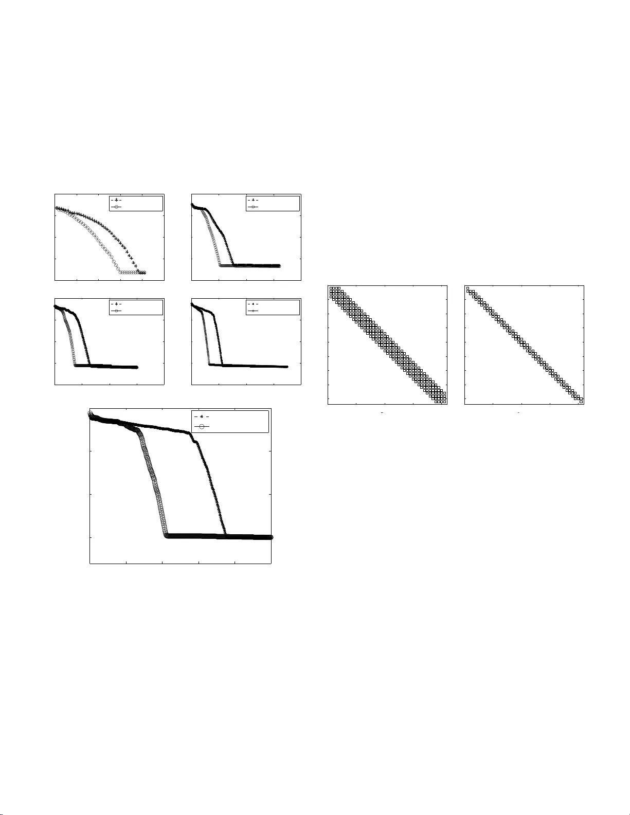
A Progressive Statistical Metho d fo r Preconditioning Matr ix-F ree Solution of High-Order Discretization o f Linear Time-Dep enden t Problems A. Ghasemi and L. K. T aylor SimCen ter: N ational Cen ter for Comp. Eng., 701 East M L King Blvd, Chattano oga, TN 3 7403 In tro duction and M otiv ati ons Consider the general form of linear time-dependent problems ∂ u ∂ t = R = L ( t, u ) = X k X i α ki ∂ k u ∂ x i k , (1) where the residual vector R contains hig h- order deriv atives of the dep endent v ariable u ( t, x 1 , x 2 , . . . , x n ) with r esp ect to independent v ar iables. Equation (1) is an abstra c t re presen- tation of a generic Partial Differential Equa tion (P DE ) in the residual form where t he linear op erator L accounts for a linear combination of the k th partial der iv ative in the i th direction, i.e. ∂ k /∂ x i k . When disc r etized using a suitable discretiza- tion metho d like Finite-Differences, Finite Element s or Finite V olume [5], the resulting equatio ns ca n be written in the fol- lowing se mi-discrete form d dt u = L u . (2) The fully dis crete from is obtained after eq.(2) is discretized in time. There are many choices av ailable for time-discretization [6]. How ever a common step in these alg orithms, which is the most costly part of the so lution, is simply an Euler implicit scheme pres e nt ed b elow u n +1 − u n ∆ t = Lu n +1 , (3) which leads to the s olution of the following system of line ar e qu ations ( I − ∆ t L ) | {z } A u n +1 = u n , (4) where A = ( I − ∆ t L ) is typically a huge spar se matrix for practical problems. F or this reas on, a dir ect solution of eq.(4) is impossible and thus an iterative algorithm is usually used for the solution. These a lg orithms rang e fro m stationar y metho ds including Jacobi, Ga us s-Seidel, SOR to more so phis- ticated K rylov subspace metho ds CG (Conjugate Gradient) and GMRES (Generalized Minimal Residual). The reader should r efer to [4] and refer ences therein for mor e detail. In this w ork , the GMRES algo rithm [1] 1 is used as the base alg o- rithm howev er the statistical preconditio ning prop os e d her e can b e readily applied to all Krylov subspace methods because they are based on matrix- vector multiplication. The imp o rtant p oint is that for many practica l pro blems the matrix A in eq .(4) is so huge that it do es not fit in the ph ysica l memory of the cur rent mac hines. This situation t yp- ically happ ens in Large E ddy Simulation (LES) or Direct Nu- merical Simulations (DNS) of a tur bulent fluid flow [8]. In this situation a full implicit solution pro cedure is avoided to preven t the pro ble m of s toring the full Ja cobian matrix. Y et still another p ossibility is av ailable by using a matrix-fre e im- plement ation [7]. In this appr oach the matrix A is never computed/stored but eq.(4) is solved b y replacing the matrix- vector pro duct in the GMRES algorithm with res idual com- putation. How ever the o nly disadv antage of this approach is that pr e c onditioning is almost impo ssible since entries a ij of A ar e not av aila ble. This is the motivation for cur r ent work where a simple statistical metho d is used to estimate A b y least-squar ing the history of ma trix-vector pro duct o btained in the GMRES algo rithm. The PS P-GMRES Algorithm The details of the P r ogre s sive Statistical Pr e conditioning for GMRES is c overed in algorithms (1) and (2) b elow. T o solve the linear system eq.(4), the original GMRE S algor ithm sta r ts as usual in algor ithm (1 ). Ho wev er when a matr ix-vector pro duct is p erformed in lines 4 a nd 11 of (1), for the given vector P x (: , i ), the result is store d in the i th column o f matrix P y , i.e. P y (: , i ). Therefore the st atistic al dataset P y versus P x is o btained pr o gr essively in a sense that the mo r e matr ix - vector pro duct is p erfo rmed the b etter dataset is obtained. Now, the primar y goa l is to find a rela tion b etw een P y and P x such tha t it has minim um error compar ed to the exac t relation P y = AP x . T his rela tio n, which is estimated using a ba nded diagona l matrix N such tha t P y ≈ NP x will be further us ed as a preconditioner in the GMRES alg orithm (1) when eq.(4) is solved for the next time step ∆ t . The a pproxi- mation of A with the banded diagonal matrix N is illustrated in fig.(1). As shown, a ll off-diagona l entries on a given rows of the or iginal huge matrix A are reduced to a banded matrix N where the matrix-vector pro duct would be cheap. This reduc- tion pro ce dur e is completely desc rib ed in algo rithm (2) us ing a mult i-r e g ressio n estimatio n o f matrix P y versus ma trix P x . As shown, the output of the GMRES algo rithm, i.e. P x and P y are sent to MREP (Multi regr essor Pr econditioner) where for d = 1, a tridiagonal estimation (three regresso rs) is en- forced. The emphasis on three regr essor mo del is based on the fact that this appro a ch leads to a tridiag onal matrix N which ca n be solved efficiently in O ( n ) FLOP s using Thomas algorithm. Th us it is exp ected that this three- regres sor m o del would save a lot when the preconditioned equa tions nee d to 1 The l east-squares is used in Ref. [1] to solve a system con taining an upp er Hessenberg matrix. How ever in this work it is used to estimate the preconditioner from a regression point of view. 1 be solved in lines 10 and 42 o f alg .(1). 1 subroutine (X, R , P x , P y ) ← PSPGMRES ( A , B, N , ǫ , n A , X 0 , n r ); 2 i ← 1; 3 for l ← 1 to n r do 4 P x (: , i ) ← X 0 , P y (: , i ) ← A X 0 ; 5 ¯ R ← B − P y (: , i ), i ← i + 1; 6 V (: , 1) ← ¯ R/ k ¯ R k ; 7 G (1) ← k ¯ R k ; 8 for k ← 1 to n A do 9 G ( k + 1) ← 0; 10 Y k ← N − 1 V (: , k ); 11 P x (: , i ) ← Y k , P y (: , i ) ← A Y k ; 12 U k ← P y (: , i ), i ← i + 1; 13 for j ← 1 to k do 14 H ( j, k ) ← V (: , j ) ′ U k ; 15 U k ← U k − H ( j, k ) V (: , j ) ; 16 end 17 H ( k + 1 , k ) ← k U k k ; 18 V (: , k + 1) ← U k / H ( k + 1 , k ); 19 for j ← 1 to k − 1 do 20 δ ← H ( j, k ); 21 H ( j, k ) ← δ C ( j ) + S ( j ) H ( j + 1 , k ); 22 H ( j + 1 , k ) ← − δ S ( j ) + C ( j ) H ( j + 1 , k ); 23 end 24 γ ← p H ( k , k ) 2 + H ( k + 1 , k ) 2 ; 25 C ( k ) ← H ( k , k ) /γ ; 26 S ( k ) ← H ( k + 1 , k ) /γ ; 27 H ( k, k ) ← γ ; 28 H ( k + 1 , k ) ← 0; 29 δ ← G ( k ); 30 G ( k ) ← C ( k ) δ + S ( k ) G ( k + 1); 31 G ( k + 1) ← − S ( k ) δ + C ( k ) G ( k + 1); 32 R ( k ) ← k G ( k + 1) k ; 33 if R ( k ) ≤ ǫ then 34 finish-flag g e ts 1; 35 break ; 36 end 37 end 38 Q ← H − 1 G ; 39 for j ← 1 to k do 40 Z k ← Z k + Q ( j ) V (: , j ); 41 end 42 X ← X 0 + N − 1 Z k ; 43 X 0 ← X ; 44 clean G, V , H , C, S ; 45 if finish-flag is set then 46 break ; 47 end 48 end Algorithm 1: The Progr essive Statistica l Pre c o nditioned GMRES algorithm (PSPGMRES) wit h p ossible restarting. As a summary , the output of the matrix- vector pro duct in the GMRES alg .(1) is stor ed in t wo matrices P x and P y which are use d a s dataset for further mo deling of the u nav ailable ma- trix A . Subseq uently , in the nex t immediate stage, the ma- trices P x and P y are used in alg. (2) where a three reg r essor s least squa re pro cedure (four unknowns) is used (d=1) to ob- tain the tridiagonal entries of the appro ximate matrix N . This matrix is g uaranteed to approximate the exact ma tr ix A with minimal r esidual. Finally the computed matrix N is used as a preconditioner in the GMRES algor ithm (1) to impro ve the conv ergence. Obviously , the mor e conv ergence of GMRES is improv ed the clos e r N to A is and vice versa. Now, it is inter- esting to see the results of this metho d in the implementation. 1 function N ← M REP ( P x , P y , d ); 2 n ← num b er of ro ws of P x ; 3 m ← num b er of columns of P x ; 4 for i ← 1 to d do 5 ( β 0 , β 1 ) ← linear fit ( P x ( i, :), P y ( i, :)); 6 N ( i, i ) ← β 1 ; 7 end 8 for i ← ( d + 1) to ( n − d ) do 9 P ∗ x ←               1 1 . . . 1  1 × m P x ( i − d, :) . . . P x ( i − 1 , :) P x ( i, :) P x ( i + 1 , :) . . . P x ( i + d, :)              ; 10 P ∗ y ← P y ( i, :); 11 N ∗ ←  P ∗ x ( P ∗ x ) ′  − 1 P ∗ x  P ∗ y ′  ; 12 for j ← 2 to 2( d + 1) do 13 N ( i, i − j − d + 1) ← N ∗ ( j ); 14 end 15 end 16 for i ← ( n − d + 1) to n do 17 ( β 0 , β 1 ) ← linear fit ( P x ( i, :), P y ( i, :)); 18 N ( i, i ) ← β 1 ; 19 end Algorithm 2: The a lg orithm for Multi-Regr essor Estima- tor of the P reconditioner (MREP). Results The a lgorithms are implement ed in a computer progra m. In a mo ck test ca se, the matrix A n × n in eq.(4) is a seven diag- onal ra ndom ma trix which is g enerated on fly in a wa y that diagonal dominance is preserved. This vector u n is just a vec- tor fro m 1 to n . The size of the system of equation, i.e. n is v aried to n = { 20 , 80 , 150 , 3 50 , 7 00 } . The structure o f the original matrix A for the ca s e 20x2 0 and the pre c o nditioner N is shown in fig.(3). As s hown for d = 1, a tridiag onal ma - trix is generated. Figure (2) co mpares the co nv ergence of the PSP-GMRES metho d with the o riginal GMRES alg o rithm. The original matrix of discretization The statistically estimated preconditioner Multivariate regression formulation Figure 1: The schematic of the statistical reduction of the sparse matrix A into the banded diagona l matrix N . As shown for ca se 20 x20, the conv ergence is decr eased 2 from 40 iterations to 30 iterations. This indicates a factor 4/3 in the sp eed-up of original algor ithm. Interestingly more impressive results would be o bta ined for larg er sys tems. Ac- cording to the s ame figure, as the size of the linear system is incr e ased, the spe e d-up ge nr ated by the PSP a lg orithm is also incr eased. As shown in fig.(2), the new statistica l pre- conditioning appr oach reduces the conv ergence of the or iginal GMRES fr om approximately 4 0 0 iterations to a pproximately 200 iter ations when A is 70 0x700 matrix! This is a numeri- cally v alidated indication of the robustness of the statistical approach. 0 10 20 30 40 50 10 −15 10 −10 10 −5 10 0 10 5 Diag. PGMRES PSP GMRES 0 50 100 150 200 10 −15 10 −10 10 −5 10 0 10 5 Diag. PGMRES PSP GMRES 0 100 200 300 400 10 −15 10 −10 10 −5 10 0 10 5 Diag. PGMRES PSP GMRES 0 200 400 600 800 10 −15 10 −10 10 −5 10 0 10 5 Diag. PGMRES PSP GMRES 0 100 200 300 400 500 10 −10 10 −5 10 0 10 5 Diag. PGMRES PSP GMRES Figure 2: The res idual norm versus num b er of GMRES itera- tions. F rom top-left to b ottom-r ig ht: 2 0x20, 80x80, 150x 150, 350x3 50 a nd 700x70 0. More Regressors and Conclusions It should b e noted that the num ber of regr essor s use d in alg.(2) was chosen to be three ( d = 1 ) in the presented im- plement ation in o rder to obtain a tridiagona l pr econditioner. How ever other alternatives migh t b e av ailable for d > 1 for future w or k s. F or example, all off-dia gonal entries might b e selected as regress ors in the initial mode l. Ther e fo re the ini- tial mo del might hav e n regres s ors. As the GMRES pr ogress and more matrix-vector multiplications a re performed, a stan- dard mo del s e lection pr o cedure, like backw ard elimination, might be used to e liminate ina ppropriate r egresso rs[3, 2]. This would result in optimum mo del which mig ht result in opti- m um sp eed-up of the conv ergence of the GMRES algo r ithm. How ever this approach has t wo exp en sive parts that should be analyzed mathematically in a s e parate pap er. The first disadv a nage is that elimination of inappropr iate regres s ors requires to ge nerate some mo de ls at star tup. This would require at le ast the cost of O ( n 3 ) fo r g enerating the first mo del using all regre s sors which is not acceptable be - cause the cos t is even hig her than so lv ing the s y stem without preconditioning! In addition, more mo dels are needed to b e created and compared to e a ch o ther dur ing this pro cedure which makes it even more exp ensive. The seco nd disa dv angate of increa sing the num ber of re- gresso rs is that the final pr econditioner matrix would not b e tridiagona l therefore the cost of solution of preconditioned system in lines 10 and 42 o f alg .(1) would increase dramati- cally in this case! 0 10 20 30 40 0 5 10 15 20 25 30 35 40 n z = 2 7 5 0 10 20 30 40 0 5 10 15 20 25 30 35 40 n z = 1 1 9 Figure 3: Left) The orig inal pattern o f the matrix. Righ t) The statistically reduced matrix used as preconditioner. The size of the matrix is n = 2 0. As a final conclusion, the three regr essor mo del presented here has alrea dy ge nerated impres s ive r esults in improving the co nvergence of the or iginal GMRES alg orithm acc o rding to fig(2). Ho wev er, there might b e situations that adding more regr essors , i.e. d > 1 would result in outstanding im- prov ements in the co nv ergence rate. It was mentioned that a backward elimination metho d is not pra c tical in this case th us a forward selection is appropriate. This situatio n should be considered more rig o rously in the future works. References [1] Y. Saad and M. H. Sch ultz, “GMRES: a generalized m inimal residual algorithm for solving nonsymmetric linear systems”, SIAM J. Sci. Stat . Comput . , July 1986, 7 ,3,Jul,1986, pp. 856-869. [2] C. Gao, “Lect ure Note Applied Statistical Methods”, Univer sity of T ennessee at Chat- tanooga, Spring 2013, h ttp://web2.utc.edu/ ~ thc544/Math4120Spring2013/Lecture%20Notes/ . [3] D. C. Mon tgomery , E. A. Pec k and G. G. Vining, “Int roduction to L inear Regre ssion Analysis 4th E d.”, Wiley-Interscience , 2006. [4] R. Barrett et. al., “T empl ates for the Solution of Linear Systems: Building B locks for Iter ative Methods”, 2nd Ed., SIAM, 1994. [5] C. Johnson, “Numer ical Solution of Part ial Differential E quations by the Finite E le- ment Method”, Dover Pub,. Jan. 2009. [6] J. C. Butche r, “Numerical Methods for O rdinary D ifferen tial Equations”, 2nd Ed., Wiley , 2008. [7] , D.A. Knoll and D.E. Keye s, “Jacobian-free N ewtonKrylov methods: a surve y of approac hes and applications”, J. Comp. Physics, 193 ,pp. 357-397, 2007. [8] M. Lesieur, O. Mtais and P . Comte, “L arge-Eddy Simulations of T urbulence”, Cam- bridge Univ. Press, 2005. 3