Distributed Clustering of Linear Bandits in Peer to Peer Networks

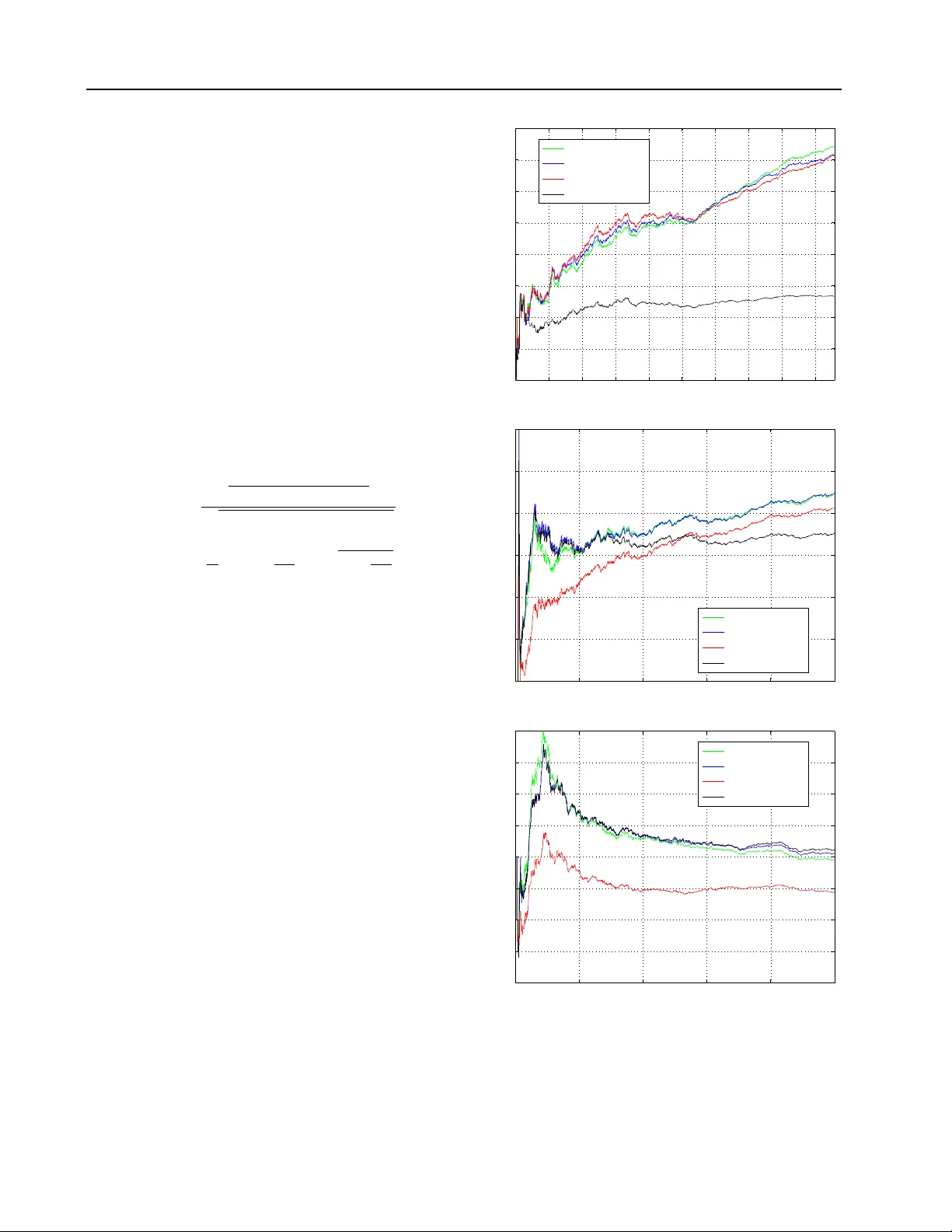
Distrib uted Clustering of Linear Bandits in P eer to P eer Networks Nathan Korda NAT H A N @ RO B O T S . O X . A C . U K MLRG, Univ ersity of Oxford Bal ´ azs Sz ¨ or ´ enyi S Z O R E N Y I . B A L A Z S @ G M A I L . C O M EE, T echnion & MT A-SZTE Research Group on Artificial Intelligence Shuai Li S H UA I L I . S L I @ G M A I L . C O M DiST A, Uni versity of Insubria Abstract W e provide tw o distributed confidence ball algo- rithms for solving linear bandit problems in peer to peer networks with limited communication ca- pabilities. For the first, we assume that all the peers are solving the same linear bandit problem, and prove that our algorithm achiev es the opti- mal asymptotic regret rate of any centralised al- gorithm that can instantly communicate informa- tion between the peers. For the second, we as- sume that there are clusters of peers solving the same bandit problem within each cluster , and we prov e that our algorithm disco vers these clusters, while achieving t he optimal asymptotic regret rate within each one. Through experiments on sev eral real-world datasets, we demonstrate the performance of proposed algorithms compared to the state-of-the-art. 1. Introduction Bandits are a class of classic optimisation problems that are fundamental to sev eral important application areas. The most prominent of these is recommendation systems, and they can also arise more generally in networks (see, e.g., (Li et al., 2013; Hao et al., 2015)). W e consider settings where a network of agents are try- ing to solve collaborativ e linear bandit problems. Sharing experience can improv e the performance of both the whole network and each agent simultaneously , while also increas- ing robustness. Howe ver , we want to av oid putting too much strain on communication channels. Communicating ev ery piece of information would just o verload these chan- Pr oceedings of the 33 rd International Conference on Machine Learning , New Y ork, NY , USA, 2016. JMLR: W&CP volume 48. Copyright 2016 by the author(s). nels. The solution we propose is a gossip-based informa- tion sharing protocol which allows information to diffuse across the network at a small cost, while also providing ro- bustness. Such a set-up would benefit, for example, a small start-up that provides some recommendation system service b ut has limited resources. Using an architecture that enables the agents (the client’ s devices) to e xchange data between each other directly and to do all the corresponding computations themselves could significantly decrease the infrastructural costs for the company . At the same time, without a central server , communicating all information instantly between agents would demand a lot of bandwidth. Multi-Agent Linear Bandits In the simplest setting we consider , all the agents are trying to solve the same un- derlying linear bandit problem. In particular , we hav e a set of nodes V , indexed by i , and representing a finite set of agents . At each time, t : • a set of actions (equiv alently , the contexts ) arriv es for each agent i , D i t ⊂ D and we assume the set D is a subset of the unit ball in R d ; • each agent, i , chooses an action (context) x i t ∈ D i t , and receiv es a r ewar d r i t = ( x i t ) T θ + ξ i t , where θ is some unknown coefficient vector , and ξ i t is some zero mean, R -subGaussian noise; • last, the agents can share information according to some protocol across a communication channel. W e define the instantaneous r e gr et at each node i , and, re- spectiv ely , the cumulative r e gr et ov er the whole netw ork to be: ρ i t :=  x i, ∗ t  T θ − E r i t , and R t := t X k =1 | V | X i =1 ρ i t , Distributed Clustering of Linear Bandits in P eer to P eer Networks where x i, ∗ t := arg max x ∈D i t x T θ . The aim of the agents is to minimise the rate of increase of cumulativ e re gret. W e also wish them to use a sharing protocol that does not im- pose much strain on the information-sharing communica- tion channel. Gossip protocol In a gossip protocol (see, e.g., (Kempe et al., 2003; Xiao et al., 2007; Jelasity et al., 2005; 2007)), in each round, an overlay protocol assigns to ev ery agent another agent, with which it can share information. After sharing, the agents aggre gate the information and, based on that, they make their corresponding decisions in the next round. In man y areas of distributed learning and compu- tation gossip protocols have offered a good compromise between low-communication costs and algorithm perfor- mance. Using such a protocol in the multi-agent bandit setting, one faces two major challenges. First, information sharing is not perfect, since each agent acquires information from only one other (randomly cho- sen) agent per round. This introduces a bias through the unav oidable doubling of data points. The solution is to mit- igate this by using a delay (typically of O (log t ) ) on the time at which information gathered is used. After this de- lay , the information is suf ficiently mixed among the agents, and the bias vanishes. Second, in order to realize this delay , it is necessary to store information in a buf fer and only use it to make decisions after the delay has been passed. In (Sz ¨ or ´ enyi et al., 2013) this was achieved by introducing an epoch structure into their algorithm, and emptying the b uf fers at the end of each epoch. The Distrib uted Confidence Ball Algorithm (DCB) W e use a gossip-based information sharing protocol to produce a distributed variant of the generic Confidence Ball (CB) algorithm, (Abbasi-Y adkori et al., 2011; Dani et al., 2008; Li et al., 2010). Our approach is similar to (Sz ¨ or ´ enyi et al., 2013) where the authors produced a distrib uted  -greedy al- gorithm for the simpler multi-armed bandit problem. How- ev er their results do not generalise easily , and thus signifi- cant ne w analysis is needed. One reason is that the linear setting introduces serious complications in the analysis of the delay ef fect mentioned in the previous paragraphs. Ad- ditionally , their algorithm is epoch-based, whereas we are using a more natural and simpler algorithmic structure. The downside is that the size of the buffers of our algorithm grow with time. Howe ver , our analyses easily transfer to the epoch approach too. As the rate of gro wth is logarith- mic, our algorithm is still ef ficient o ver a v ery long time- scale. The simplifying assumption so far is that all agents are solving the same underlying bandit problem, i.e. finding the same unkno wn θ -vector . This, ho we ver , is often unre- alistic, and so we relax it in our next setup. While it may hav e uses in special cases, DCB and its analysis can be con- sidered as a base for providing an algorithm in this more realistic setup, where some variation in θ is allowed across the network. Clustered Linear Bandits Proposed in (Gentile et al., 2014; Li et al., 2016a;b), this has recently proved to be a very successful model for recommendation problems with massiv e numbers of users. It comprises a multi-agent linear bandit model agents’ θ -vectors are allo wed to v ary across a clustering. This clustering presents an additional challenge to find the groups of agents sharing the same underlying bandit problem before information sharing can accelerate the learning process. F ormally , let { U k } k =1 ,...,M be a clus- tering of V , assume some coefficient vector θ k for each k , and let for agent i ∈ U k the reward of action x i t be given by r i t = ( x i t ) T θ k + ξ i t . Both clusters and coef ficient v ectors are assumed to be ini- tially unknown, and so need to be learnt on the fly . The Distributed Clustering Confidence Ball Algorithm (DCCB) The paper (Gentile et al., 2014) proposes the ini- tial centralised approach to the problem of clustering linear bandits. Their approach is to begin with a single cluster , and then incrementally prune edges when the available in- formation suggests that tw o agents belong to different clus- ters. W e sho w ho w to use a gossip-based protocol to gi v e a distributed v ariant of this algorithm, which we call DCCB. Our main contributions In Theorems 1 and 6 we sho w our algorithms DCB and DCCB achiev e, in the multi-agent and clustered setting, respectiv ely , near-optimal improve- ments in the regret rates. In particular , they are of order almost p | V | better than applying CB without informa- tion sharing, while still keeping communication cost low . And our findings are demonstrated by experiments on real- world benchmark data. 2. Linear Bandits and the DCB Algorithm The generic Confidence Ball (CB) algorithm is designed for a single agent linear bandit problem (i.e. | V | = 1 ). The algorithm maintains a confidence ball C t ⊂ R d within which it believ es the true parameter θ lies with high prob- ability . This confidence ball is computed from the obser- vation pairs, ( x k , r k ) k =1 ,...,t (for the sak e of simplicity , we dropped the agent index, i ). T ypically , the cov ariance ma- trix A t = P t k =1 x k x T k and b -vector , b t = P t k =1 r k x k , are sufficient statistics to characterise this confidence ball. Then, giv en its current action set, D t , the agent selects the optimistic action, assuming that the true parameter sits in C t , i.e. ( x t , ∼ ) = arg max ( x,θ 0 ) ∈D t × C t { x T θ 0 } . Pseudo- code for CB is giv en in the Appendix A.1. Distributed Clustering of Linear Bandits in P eer to P eer Networks Gossip Sharing Protocol for DCB W e assume that the agents are sharing across a peer to peer network, i.e. ev ery agent can share information with e very other agent, but that ev ery agent can communicate with only one other agent per round. In our algorithms, each agent, i , needs to maintain (1) a buf fer (an ordered set) A i t of co v ariance matrices and an active cov ariance matrix ˜ A i t , (2) a buffer B i t of b-vectors and an active b -v ector ˜ b i t , Initially , we set, for all i ∈ V , ˜ A i 0 = I , ˜ b i 0 = 0 . These active objects are used by the algorithm as suf fi- cient statistics from which to calculate confidence balls, and summarise only information gathered before or during time τ ( t ) , where τ is an arbitrary monotonically increasing function satisfying τ ( t ) < t . The b uffers are initially set to A i 0 = ∅ , and B i 0 = ∅ . For each t > 1 , each agent, i , shares and updates its buf fers as follows: (1) a random permutation, σ , of the numbers 1 , . . . , | V | is chosen uniformly at random in a decentralised manner among the agents, 1 (2) the buffers of i are then updated by averaging its buf fers with those of σ ( i ) , and then extending them us- ing their current observations 2 A i t +1 =  1 2 ( A i t + A σ ( i ) t )  ◦  x i t +1  x i t +1  T  , B i t +1 =  1 2 ( B i t + B σ ( i ) t )  ◦  r i t +1 x i t +1   , ˜ A i t +1 = ˜ A i t + ˜ A σ ( i ) t , and ˜ b i t +1 = ˜ b i t + ˜ b σ ( i ) t . (3) if the length |A i t +1 | exceeds t − τ ( t ) , the first element of A i t +1 is added to ˜ A i t +1 and deleted from A i t +1 . B i t +1 and ˜ b i t +1 are treated similarly . In this way , each buf fer remains of size at most t − τ ( t ) , and contains only information g athered after time τ ( t ) . The re- sult is that, after t rounds of sharing, the current co variance matrices and b-vectors used by the algorithm to mak e deci- sions hav e the form: ˜ A i t := I + τ ( t ) X t 0 =1 | V | X i 0 =1 w i 0 ,t 0 i,t x i 0 t 0 x i 0 t 0 T , and ˜ b i t := τ ( t ) X t 0 =1 | V | X i 0 =1 w i 0 ,t 0 i,t r i 0 t 0 x i 0 t 0 . where the weights w i 0 ,t 0 i,t are random variables which are unknown to the algorithm. Importantly for our analysis, as 1 This can be achiev ed in a v ariety of ways. 2 The ◦ symbol denotes the concatenation operation on two ordered sets: if x = ( a, b, c ) and y = ( d, e, f ) , then x ◦ y = ( a, b, c, d, e, f ) , and y ◦ x = ( d, e, f , a, b, c ) . a result of the ov erlay protocol’ s uniformly random choice of σ , they are identically distributed ( i.d. ) for each fixed pair ( t, t 0 ) , and P i 0 ∈ V w i 0 ,t 0 i,t = | V | . If information sharing was perfect at each time step, then the current co v ariance matrix could be computed using all the information gath- ered by all the agents, and would be: A t := I + | V | X i 0 =1 t X t 0 =1 x i 0 t 0  x i 0 t 0  T . (1) DCB algorithm The OFUL algorithm (Abbasi-Y adkori et al., 2011) is an improv ement of the confidence ball al- gorithm from (Dani et al., 2008), which assumes that the confidence balls C t can be characterised by A t and b t . In the DCB algorithm, each agent i ∈ V maintains a confi- dence ball C i t for the unkno wn parameter θ as in the OFUL algorithm, b ut calculated from ˜ A i t and ˜ b i t . It then chooses its action, x i t , to satisfy ( x i t , θ i t ) = arg max ( x,θ ) ∈D i t × C i t x T θ , and receiv es a re ward r i t . Finally , it shares its information buf fer according to the sharing protocol above. Pseudo- code for DCB is giv en in Appendix A.1, and in Algorithm 1. 2.1. Results for DCB Theorem 1. Let τ ( · ) : t → 4 log ( | V | 3 2 t ) . Then, with pr ob- ability 1 − δ , the re gret of DCB is bounded by R t ≤ ( N ( δ ) | V | + ν ( | V | , d, t )) k θ k 2 + 4 e 2 ( β ( t ) + 4 R ) r | V | t ln  (1 + | V | t/d ) d  , wher e ν ( | V | , d, t ) := ( d + 1) d 2 (4 | V | ln( | V | 3 2 t )) 3 , N ( δ ) := √ 3 / ((1 − 2 − 1 4 ) √ δ ) , and β ( t ) := R v u u t ln (1 + | V | t/d ) d δ ! + k θ k 2 . (2) The term ν ( t, | V | , d ) describes the loss compared to the centralised algorithm due to the delay in using informa- tion, while N ( δ ) | V | describes the loss due to the incom- plete mixing of the data across the network. If the agents implement CB independently and do not share any information, which we call CB- NoSharing , then it fol- lows from the results in (Abbasi-Y adkori et al., 2011), the equiv alent regret bound would be R t ≤| V | β ( t ) q t ln ((1 + t/d ) d ) (3) Comparing Theorem 1 with (3) tells us that, after an initial “burn in” period, the gain in regret performance of DCB ov er CB- NoSharing is of order almost p | V | . Distributed Clustering of Linear Bandits in P eer to P eer Networks Corollary 2. W e can reco ver a bound in expectation from Theor em 1, by using the value δ = 1 / p | V | t : E [ R t ] ≤ O ( t 1 4 ) + p | V | t k θ k 2 + 4 e 2 R r ln  (1 + | V | t/d ) d p | V | t  + k θ k 2 + 4 R ! × q | V | t ln ((1 + | V | t/d ) d ) . This shows that DCB exhibits asymptotically optimal re- gret performance, up to log factors, in comparison with any algorithm that can share its information perfectly between agents at each round. C O M M U N I C A T I O N C O M P L E X I T Y If the agents communicate their information to each other at each round without a central serv er , then every agent w ould need to communicate their chosen action and rew ard to e v- ery other agent at each round, giving a communication cost of order d | V | 2 per-round. W e call such an algorithm CB- InstSharing . Under the gossip protocol we propose each agent requires at most O ( l og 2 ( | V | t ) d 2 | V | ) bits to be com- municated per round. Therefore, a significant communica- tion cost reduction is gained when log ( | V | t ) d  | V | . Using an epoch-based approach, as in (Sz ¨ or ´ enyi et al., 2013), the per -round communication cost of the gossip pro- tocol becomes O ( d 2 | V | ) . This improves efficiency over any horizon, requiring only that d  | V | , and the proofs of the regret performance are simple modifications of those for DCB. Howe ver , in comparison with growing buf fers this is only an issue after O (exp( | V | )) number of rounds, and typically | V | is large. While the DCB has a clear communication advantage ov er CB- InstSharing , there are other potential approaches to this problem. For example, instead of randomised neighbour sharing one can use a deterministic protocol such as Round- Robin (RR), which can hav e the same low communication costs as DCB. Howe ver , the regret bound for RR suffers from a naturally larger delay in the network than DCB. Moreov er , attempting to track potential doubling of data points when using a gossip protocol, instead of employing a delay , leads back to a communication cost of order | V | 2 per round. More detail is included in Appendix A.2. P R O O F O F T H E O R E M 1 In the analysis we show that the bias introduced by imper- fect information sharing is mitigated by delaying the in- clusion of the data in the estimation of the parameter θ . The proof builds on the analysis in (Abbasi-Y adkori et al., 2011). The emphasis here is to show how to handle the extra dif ficulty stemming from imperfect information shar- ing, which results in the influence of the various re wards at the v arious peers being unbalanced and appearing with a random delay . Proofs of the Lemmas 3 and 4, and of Proposition 1 are crucial, but technical, and are deferred to Appendix A.3. Step 1: Define modified confidence ellipsoids. First we need a version of the confidence ellipsoid theorem given in (Abbasi-Y adk ori et al., 2011) that incorporates the bias introduced by the random weights: Proposition 1. Let δ > 0 , ˜ θ i t := ( ˜ A i t ) − 1 ˜ b i t , W ( τ ) := max { w i 0 ,t 0 i,t : t, t 0 ≤ τ , i, i 0 ∈ V } , and let C i t :=  x ∈ R d : k ˜ θ i t − x k ˜ A i t ≤ k θ k 2 (4) + W ( τ ( t )) R r 2 log  det( ˜ A i t ) 1 2 /δ   . Then with pr obability 1 − δ , θ ∈ C i t . In the rest of the proof we assume that θ ∈ C i t . Step 2: Instantaneous regret decomposition. Denote by ( x i t , θ i t ) = arg max x ∈ D i t ,y ∈ C i t x T y . Then we can de- compose the instantaneous re gret, follo wing a classic ar gu- ment (see the proof of Theorem 3 in (Abbasi-Y adk ori et al., 2011)): ρ i t =  x i, ∗ t  T θ − ( x i t ) T θ ≤  x i t  T θ i t − ( x i t ) T θ =  x i t  T h θ i t − ˜ θ i t  +  ˜ θ i t − θ i ≤ k x i t k ( ˜ A i t ) − 1     θ i t − ˜ θ i t    ˜ A i t +    ˜ θ i t − θ    ˜ A i t  (5) Step 3: Control the bias. The norm differences inside the square brackets of the regret decomposition are bounded through (4) in terms of the matrices ˜ A i t . W e would like, instead, to hav e the regret decomposition in terms of the matrix A t (which is defined in (1)). T o this end, we giv e some lemmas sho wing that using the matrices ˜ A i t is almost the same as using A t . These lemmas inv olv e elementary matrix analysis, but are crucial for understanding the im- pact of imperfect information sharing on the final regret bounds. Step 3a: Control the bias coming fr om the weight im- balance. Lemma 3 (Bound on the influence of general weights) . F or all i ∈ V and t > 0 , k x i t k 2 ( ˜ A i t ) − 1 ≤ e P τ ( t ) t 0 =1 P | V | i 0 =1    w i 0 ,t 0 i,t − 1    k x i t k 2 ( A τ ( t ) ) − 1 , and det  ˜ A i t  ≤ e P τ ( t ) t 0 =1 P | V | i 0 =1    w i 0 ,t 0 i,t − 1    det  A τ ( t )  . Using Lemma 4 in (Sz ¨ or ´ enyi et al., 2013), by exploiting the random weights are identically distributed ( i.d. ) for each Distributed Clustering of Linear Bandits in P eer to P eer Networks fixed pair ( t, t 0 ) , and P i 0 ∈ V w i 0 ,t 0 i,t = | V | under our gos- sip protocol, we can control the random exponential con- stant in Lemma 3, and the upper bound W ( T ) using the Chernoff-Hoef fding bound: Lemma 4 (Bound on the influence of weights under our sharing protocol) . F ix some constants 0 < δ t 0 < 1 . Then with pr obability 1 − P τ ( t ) t 0 =1 δ t 0 | V | X i 0 =1 τ ( t ) X t 0 =1    w i 0 ,t 0 i,t − 1    ≤ | V | 3 2 τ ( t ) X t 0 =1  2 ( t − t 0 ) δ t 0  − 1 2 , and W ( T ) ≤ 1 + max 1 ≤ t 0 ≤ τ ( t )  | V | 3 2  2 ( t − t 0 ) δ t 0  − 1 2  . In particular, for any δ ∈ (0 , 1) , choosing δ t 0 = δ 2 t 0 − t 2 , with probability 1 − δ / ( | V | 3 t 2 (1 − 2 − 1 / 2 )) we hav e | V | X i 0 =1 τ ( t ) X t 0 =1    w i 0 ,t 0 i,t − 1    ≤ 1 (1 − 2 − 1 4 ) t √ δ , and W ( τ ( t )) ≤ 1 + | V | 3 2 t √ δ . (6) Thus Lemma 3 and 4 give us control over the bias intro- duced by the imperfect information sharing. Combining them with Equations (4) and (5) we find that with probabil- ity 1 − δ / ( | V | 3 t 2 (1 − 2 − 1 / 2 )) : ρ i t ≤ 2 e C ( t ) k x i t k  A i τ ( t )  − 1 (1 + C ( t )) (7) × " R r 2 log  e C ( t ) det  A τ ( t )  1 2 δ − 1  + k θ k # where C ( t ) := 1 / (1 − 2 − 1 / 4 ) t √ δ Step 3b: Control the bias coming from the delay . Next, we need to control the bias introduced from leaving out the last 4 log( | V | 3 / 2 t ) time steps from the confidence ball estimation calculation: Proposition 2. Ther e can be at most ν ( k ) := (4 | V | log ( | V | 3 / 2 k )) 3 ( d + 1) d ( tr ( A 0 ) + 1) (8) pairs ( i, k ) ∈ 1 , . . . , | V | × { 1 , . . . , t } for which one of k x i k k 2 A − 1 τ ( k ) ≥ e k x i k k 2 ( A k − 1 + P i − 1 j =1 x j k ( x j k ) T ) − 1 , or det  A τ ( k )  ≥ e det   A k − 1 + i − 1 X j =1 x j k ( x j k ) T   holds. Step 4: Choose constants and sum the simple regr et. Defining a constant N ( δ ) := 1 (1 − 2 − 1 4 ) √ δ , we hav e, for all k ≥ N ( δ ) , C ( k ) ≤ 1 , and so, by (7) with probability 1 − ( | V | k ) − 2 δ / (1 − 2 − 1 / 2 ) ρ i k ≤ 2 e k x i k k A − 1 τ ( k ) (9) ×    2 R v u u u t 2 log   e det  A τ ( k )  1 2 δ   + k θ k 2    . Now , first applying Cauchy-Schwarz, then step 3b from abov e together with (9), and finally Lemma 11 from (Abbasi-Y adkori et al., 2011) yields that, with probability 1 −  1 + P ∞ t =1 ( | V | t ) − 2 / (1 − 2 − 1 / 2 )  δ ≥ 1 − 3 δ , R t ≤ N ( δ ) | V |k θ k 2 +   | V | t t X t 0 = N ( δ ) | V | X i =1  ρ i t 0  2   1 2 ≤ ( N ( δ ) | V | + ν ( | V | , d, t )) k θ k 2 + 4 e 2 ( β ( t ) + 2 R ) " | V | t t X t 0 =1 M X i =1 k x i t k 2 ( A t ) − 1 # 1 2 ≤ ( N ( δ ) | V | + ν ( | V | , d, t )) k θ k 2 + 4 e 2 ( β ( t ) + 2 R ) p | V | t (2 log (det ( A t ))) , where β ( · ) is as defined in (2). Replacing δ with δ/ 3 fin- ishes the proof. P R O O F O F P RO P O S I T I O N 2 This proof forms the major innovation in the proof of The- orem 1. Let ( y k ) k ≥ 1 be any sequence of vectors such that k y k k 2 ≤ 1 for all k , and let B n := B 0 + P n k =1 y k y T k , where B 0 is some positiv e definite matrix. Lemma 5. F or all t > 0 , and for any c ∈ (0 , 1) , we have    n k ∈ { 1 , 2 , . . . } : k y k k 2 B − 1 k − 1 > c o    ≤ ( d + c ) d ( tr ( B − 1 0 ) − c ) /c 2 , Pr oof. W e begin by sho wing that, for an y c ∈ (0 , 1) k y k k 2 B − 1 k − 1 > c (10) can be true for only 2 dc − 3 different k . Indeed, let us suppose that (10) is true for some k . Let ( e ( k − 1) i ) 1 ≤ i ≤ d be the orthonormal eigenbasis for B k − 1 , and, therefore, also for B − 1 k − 1 , and write y k = P d i =1 α i e i . Let, also, ( λ ( k − 1) i ) be the eigen v alues for B k − 1 . Then, c < y T k B − 1 k − 1 y k = d X i =1 α 2 i λ ( k − 1) i ≤ tr ( B − 1 k − 1 ) , = ⇒ ∃ j ∈ { 1 , . . . , d } : α 2 j λ ( k − 1) j , 1 λ ( k − 1) j > c d , Distributed Clustering of Linear Bandits in P eer to P eer Networks where we ha ve used that α 2 i < 1 for all i , since k y k k 2 < 1 . Now , tr ( B − 1 k − 1 ) − tr ( B − 1 k ) = tr ( B − 1 k − 1 ) − tr (( B k − 1 + y k y T k ) − 1 ) > tr ( B − 1 k − 1 ) − tr (( B k − 1 + α 2 j e j e T j ) − 1 ) = 1 λ ( k − 1) j − 1 λ ( k − 1) j + α 2 j = α 2 j λ ( k − 1) j ( λ ( k − 1) j + α 2 j ) >  d 2 c − 2 + dc − 1  − 1 > c 2 d ( d + c ) So we hav e sho wn that (10) implies that tr ( B − 1 k − 1 ) > c and tr ( B − 1 k − 1 ) − tr ( B − 1 k ) > c 2 d ( d + c ) . Since tr ( B − 1 0 ) ≥ tr ( B − 1 k − 1 ) ≥ tr ( B − 1 k ) ≥ 0 for all k , it follows that (10) can be true for at most ( d + c ) d ( tr ( B − 1 0 ) − c ) c − 2 different k . Now , using an ar gument similar to the proof of Lemma 3, for all k < t k y k +1 k B − 1 τ ( k ) ≤ e P k s = τ ( k )+1 k y s +1 k B − 1 s k y k +1 k B − 1 k , and det  B τ ( t )  ≤ e P t k = τ ( t )+1 k y k k 2 B − 1 k det ( B t ) . Therefore, k y k +1 k B − 1 τ ( k ) ≥ c k y k +1 k B − 1 k or det( B τ ( k ) ) ≥ c det( B k ) = ⇒ k − 1 X s = τ ( k ) k y s +1 k B − 1 s ≥ ln( c ) Howe ver , according to Lemma 5, there can be at most ν ( t ) :=  d + ln( c ) ∆( t )  d  tr  B − 1 0  − ln( c ) ∆( t )   ∆( t ) ln( c )  2 times s ∈ { 1 , . . . , t } , such that k y s +1 k B − 1 s ≥ ln( c ) / ∆( t ) , where ∆( t ) := max 1 ≤ k ≤ t { k − τ ( k ) } . Hence P k s = τ ( j )+1 k y s +1 k − 1 B s ≥ ln( c ) is true for at most ∆( t ) ν ( | V | , d, t ) indices k ∈ { 1 , . . . , t } . Finally , we finish by setting ( y k ) k ≥ 1 = ◦ t ≥ 1 ( x i t ) | V | i =1 . 3. Clustering and the DCCB Algorithm W e no w incorporate distributed clustering into the DCB al- gorithm. The analysis of DCB forms the backbone of the analysis of DCCB. DCCB Pruning Protocol In order to run DCCB, each agent i must maintain some local information buf fers in addition to those used for DCB. These are: Algorithm 1 Distributed Clustering Confidence Ball Input: Size of netw ork | V | , τ : t → t − 4 log 2 t, α, λ Initialization: ∀ i ∈ V , set ˜ A i 0 = I d , ˜ b i 0 = 0 , A i 0 = B i 0 = ∅ , and V i 0 = V . for t = 0 , . . . ∞ do Draw a random permutation σ of { 1 , . . . , V } respect- ing the current local clusters for i = 1 , . . . , | V | do Receiv e action set D i t and construct the confidence ball C i t using ˜ A i t and ˜ b i t Choose action and recei ve r eward: Find ( x i t +1 , ∗ ) = arg max ( x, ˜ θ ) ∈D i t × C i t x T ˜ θ , and get rew ard r i t +1 from context x i t +1 . Share and update information b uffers: if k ˆ θ i local − ˆ θ j local k > c thresh λ ( t ) Update local cluster: V i t +1 = V i t \ { σ ( i ) } , V σ ( i ) t +1 = V σ ( i ) t \ { i } , and reset according to (13) elseif V i t = V σ ( i ) t Set A i t +1 =  1 2 ( A i t + A σ ( i ) t )  ◦ ( x i t +1  x i t +1  T ) and B i t +1 =  1 2 ( B i t + B σ ( i ) t )  ◦ ( r i t +1 x i t +1 ) else Update: Set A i t +1 = A i t ◦ ( x i t +1  x i t +1  T ) and B i t +1 = B i t ◦ ( r i t +1 x i t +1 ) endif Update local estimator: A i local,t +1 = A i local,t + x i t +1  x i t +1  T , b i local,t +1 = b i local,t + r i t +1 x i t +1 , and ˆ θ local,t +1 =  A i local,t +1  − 1 b i local,t +1 if |A i t +1 | > t − τ ( t ) set ˜ A i t +1 = ˜ A i t + A i t +1 (1) , A i t +1 = A i t +1 \ A i t +1 (1) . Similarly for B i t +1 . end for end for (1) a local co v ariance matrix A i local = A i local,t , a local b- vector b i local = b i local,t , (2) and a local neighbour set V i t . The local cov ariance matrix and b-vector are updated as if the agent was applying the generic (single agent) confi- dence ball algorithm: A i local, 0 = A 0 , b i local, 0 = 0 , A i local,t = x i t ( x i t ) T + A i local,t − 1 , and b i local,t = r i t x i t + b i local,t − 1 . DCCB Algorithm Each agent’ s local neighbour set V i t is initially set to V . At each time step t , agent i contacts one other agent, j , at random from V i t , and both decide whether they do or do not belong to the same cluster . T o do this Distributed Clustering of Linear Bandits in P eer to P eer Networks they share local estimates, ˆ θ i t = A i local,t − 1 b i local,t and ˆ θ j t = A j local,t − 1 b j local,t , of the unknown parameter of the bandit problem they are solving, and see if they are further apart than a threshold function c = c thresh λ ( t ) , so that if k ˆ θ i t − ˆ θ j t k 2 ≥ c thresh λ ( t ) , (11) then V i t +1 = V i t \ { j } and V j t +1 = V j t \ { i } . Here λ is a parameter of an extra assumption that is needed, as in (Gentile et al., 2014), about the process generating the context sets D i t : (A) Each context set D i t = { x k } k is finite and contains i.i.d. random vectors such that for all, k , k x k k ≤ 1 and E ( x k x T k ) is full rank, with minimal eigen v alue λ > 0 . W e define c thresh λ ( t ) , as in (Gentile et al., 2014), by c thresh λ ( t ) := R p 2 d log ( t ) + 2 log(2 /δ ) + 1 p 1 + max { A λ ( t, δ / (4 d )) , 0 } (12) where A λ ( t, δ ) := λt δ − 8 log t +3 δ − 2 q t log t +3 δ . The DCCB algorithm is pretty much the same as the DCB algorithm, except that it also applies the pruning protocol described. In particular , each agent, i , when sharing its information with another , j , has three possible actions: (1) if (11) is not satisfied and V i t = V j t , then the agents share simply as in the DCB algorithm; (2) if (11) is not satisfied but V i t 6 = V j t , then no sharing or pruning occurs. (3) if (11) is satisfied, then both agents remove each other from their neighbour sets and reset their buf fers and activ e matrices so that A i = (0 , 0 , . . . , A i local ) , B i = (0 , 0 , . . . , b i local ) , and ˜ A i = A i local , ˜ b i = b i local , (13) and similarly for agent j . It is proved in the theorem below , that under this sharing and pruning mechanism, in high probability after some fi- nite time each agent i finds its true cluster , i.e. V i t = U k . Moreov er , since the algorithm resets to its local informa- tion each time a pruning occurs, once the true clusters ha ve been identified, each cluster shares only information gath- ered within that cluster , thus a v oiding introducing a bias by sharing information gathered from outside the cluster be- fore the clustering has been identified. Full pseudo-code for the DCCB algorithm is given in Algorithm 1, and the dif- ferences with the DCB algorithm are highlighted in blue. Distrib uted Clustering of Linear Bandits in P eer to P eer Netw orks the y share local estimates, ˆ ✓ i t = A i lo c a l, t  1 b i lo c a l, t and ˆ ✓ j t = A j lo c a l, t  1 b j lo c a l , t , of the unkno wn parameter of the bandit problem the y are solving, and see if the y are further apart than a threshold function c = c t h r es h  ( t ) , so that if k ˆ ✓ i t  ˆ ✓ j t k 2  c t h r es h  ( t ) , (11) then V i t +1 = V i t \{ j } and V j t +1 = V j t \{ i } . Here  is a parameter of an e xtra assumption that is needed, as in (Gentile et al., 2014), about the process generating the conte xt sets D i t : (A) Each conte xt set D i t = { x k } k is finite and contains i.i.d. random v ectors such that for all, k , k x k k 1 and E ( x k x T k ) is full rank, with minimal eigen v alue  > 0 . W e define c t h r es h  ( t ) , as in (Gentile et al., 2014), by c t h r es h  ( t ): = R p 2 d l og ( t ) + 2 l og ( 2 /  )+1 p 1 + m ax { A  ( t,  / (4 d )) , 0 } (12) where A  ( t,  ): =  t   8 l og t +3   2 q t l og t +3  . The DCCB algorithm is pretty much the same as the DCB algorithm, e xcept that it also applies the pruning protocol described. In particular , each agent, i , when sharing its information with another , j , has three possible actions: (1) if (11) is not satisfied and V i t = V j t , then the agents share simply as in the DCB algorithm; (2) if (11) is satisfied, then both agents remo v e each other from their neighbour sets and reset their b uf fers and acti v e matrices so that A i =( 0 , 0 ,. .., A i lo c a l ) , B i =( 0 , 0 ,. .., b i lo c a l ) , and ˜ A i = A i lo c a l , ˜ b i = b i lo c a l , (13) and similarly for agent j . (3) if (11) is not satisfied b ut V i t 6 = V j t , then no sharing or pruning occurs. It is pro v ed in the theorem belo w , that under this sharing and pruning mechanism, in high probability after some fi- nite time each agent i finds its true cluster , i.e. V i t = U k . Moreo v er , since the algorithm resets to its local informa- tion each time a pruning occurs, once the true clusters ha v e been identified, each cluster shares only information g ath- ered within that cluster , thus a v oiding introducing a bias by sharing information g athered from outside the cluster be- fore the clustering has been identified. Full pseudo-code for the DCCB algorit hm is gi v en in Algorithm 1, and the dif- ferences with the DCB algorithm are highlighted in blue. 1000 2000 3000 4000 5000 6000 7000 8000 9000 0 0.5 1 1.5 2 2.5 3 3.5 4 Rounds Ratio of Cum. Rewards of Alg. against RAN Delicious Dataset DCCB CLUB CB − NoSharing CB − InstSharing 0 2000 4000 6000 8000 10000 1 2 3 4 5 6 7 Rounds Ratio of Cum. Rewards of Alg. against RAN LastFM Dataset DCCB CLUB CB − NoSharing CB − InstSharing 0 2000 4000 6000 8000 10000 0 0.5 1 1.5 2 2.5 3 3.5 4 Rounds Ratio of Cum. Rewards of Alg. against RAN MovieLens Dataset DCCB CLUB CB − NoSharing CB − InstSharing Figure 1. Here we plot the performance of DCCB i n comparison to CLUB, CB- NoSharing and CB- InstSharing . The plots sho w the ratio of cum ulati v e re w ards achie v ed by the algorithms to the cumulati v e re w ards achie v ed by the random algorithm. Figure 1. Here we plot the performance of DCCB in comparison to CLUB, CB- NoSharing and CB- InstSharing . The plots sho w the ratio of cumulative rew ards achiev ed by the algorithms to the cumulativ e re wards achie ved by the random algorithm. Distributed Clustering of Linear Bandits in P eer to P eer Networks 3.1. Results for DCCB Theorem 6. Assume that (A) holds, and let γ denote the smallest distance between the bandit parameters θ k . Then ther e exists a constant C = C ( γ , | V | , λ, δ ) , such that with pr obability 1 − δ the total cumulative re gr et of cluster k when the agents employ DCCB is bounded by R t ≤  max n √ 2 N ( δ ) , C + 4 log 2 ( | V | 3 2 C ) o | U k | + ν ( | U k | , d, t )  k θ k 2 + 4 e ( β ( t ) + 3 R ) r | U k | t ln  (1 + | U k | t/d ) d  , wher e N and ν are as defined in Theor em 1, and β ( t ) := R r 2 ln  (1 + | U k | t/d ) d  + k θ k 2 . The constant C ( γ , | V | , λ, δ ) is the time that you have to wait for the true clustering to ha ve been identified, The analysis follows the following scheme: When the true clusters hav e been correctly identified by all nodes, within each cluster the algorithm, and thus the analysis, reduces to the case of Section 2.1. W e adapt results from (Gentile et al., 2014) to sho w how long it will be before the true clusters are identified, in high probability . The proof is de- ferred to Appendices A.4 and A.5. 4. Experiments and Discussion Experiments W e closely implemented the experimental setting and dataset construction principles used in (Li et al., 2016a;b), and for a detailed description of this we refer the reader to (Li et al., 2016a). W e ev aluated DCCB on three real-world datasets against its centralised counter- part CLUB, and against the benchmarks used therein, CB- NoSharing , and CB- InstSharing . The LastFM dataset com- prises of 91 users, each of which appear at least 95 times. The Delicious dataset has 87 users, each of which appear at least 95 times. The MovieLens dataset contains 100 users, each of which appears at least 250 times. The performance was measured using the ratio of cumulati ve re ward of each algorithm to that of the predictor which chooses a random action at each time step. This is plotted in in Figure 1. From the experimental results it is clear that DCCB per- forms comparably to CLUB in practice, and both outper- form CB- NoSharing , and CB- InstSharing . Relationship to existing literature There are several strands of research that are rele v ant and complimentary to this work. First, there is a lar ge literature on single agent linear bandits, and other more, or less complicated ban- dit problem settings. There is already w ork on distrib uted approaches to multi-agent, multi-armed bandits, not least (Sz ¨ or ´ enyi et al., 2013) which examines  -greedy strategies ov er a peer to peer netw ork, and provided an initial inspira- tion for this current work. The paper (Kalathil et al., 2014) examines the extreme case when there is no communication channel across which the agents can communicate, and all communication must be performed through observation of action choices alone. Another approach to the multi-armed bandit case, (Nayyar et al., 2015), directly incorporates the communication cost into the regret. Second, there are sev eral recent advances regarding the state-of-the-art methods for clustering of bandits. The work (Li et al., 2016a) is a faster variant of (Gentile et al., 2014) which adopt the strategy of boosted training stage. In (Li et al., 2016b) the authors not only cluster the users, but also cluster the items under collaborati ve filtering case with a sharp regret analysis. Finally , the paper (T ekin & van der Schaar, 2013) treats a setting similar to ours in which agents attempt to solve contextual bandit problems in a distributed setting. They present two algorithms, one of which is a distributed ver - sion of the approach taken in (Slivkins, 2014), and show that they achieve at least as good asymptotic regret perfor- mance in the distributed approach as the centralised algo- rithm achie ves. Howe ver , rather than sharing information across a limited communication channel, they allow each agent only to ask another agent to choose their action for them. This difference in our settings is reflected worse re- gret bounds, which are of order Ω( T 2 / 3 ) at best. Discussion Our analysis is tailored to adapt proofs from (Abbasi-Y adkori et al., 2011) about generic confidence ball algorithms to a distributed setting. Howe ver many of the elements of these proofs, including Propositions 1 and 2 could be reused to provide similar asymptotic re gret guar- antees for the distributed versions of other bandit algo- rithms, e.g., the Thompson sampling algorithms, (Agrawal & Goyal, 2013; Kaufmann et al., 2012; Russo & V an Roy, 2014). Both DCB and DCCB are synchronous algorithms. The work on distributed computation through gossip algorithms in (Boyd et al., 2006) could alle viate this issue. The current pruning algorithm for DCCB guarantees that techniques from (Sz ¨ or ´ enyi et al., 2013) can be applied to our algo- rithms. Howe ver the results in (Boyd et al., 2006) are more powerful, and could be used ev en when the agents only identify a sub-network of the true clustering. Furthermore, there are other e xisting interesting algorithms for performing clustering of bandits for recommender sys- tems, such as COFIB A in (Li et al., 2016b). It would be in- teresting to understand how general the techniques applied here to CLUB are. Distributed Clustering of Linear Bandits in P eer to P eer Networks Acknowledgments W e would like to thank the anonymous re vie wers for their helpful comments. W e would also like to thank Gerg- ley Neu for very useful discussions. NK thanks the sup- port from EPSRC Autonomous Intelligent Systems project EP/I011587. SL thanks the support from MIUR, QCRI- HBKU, Amazon Research Grant and Tsinghua Univ ersity . The research leading to these results has receiv ed funding from the European Research Council under the European Union’ s Sev enth Frame work Programme (FP/2007-2013) / ERC Grant Agreement n. 306638. References Abbasi-Y adkori, Y asin, P ´ al, D ´ avid, and Szepesv ´ ari, Csaba. Improv ed algorithms for linear stochastic bandits. In NIPS , pp. 2312–2320, 2011. Agrawal, Shipra and Goyal, Navin. Thompson sampling for contextual bandits with linear payoffs. In ICML , 2013. Boyd, Stephen, Ghosh, Arpita, Prabhakar, Balaji, and Shah, De v a vrat. Randomized gossip algorithms. IEEE/A CM T r ansactions on Networking (T ON) , 14(SI): 2508–2530, 2006. Dani, V arsha, Hayes, Thomas P , and Kakade, Sham M. Stochastic linear optimization under bandit feedback. In COLT , pp. 355–366, 2008. Gentile, Claudio, Li, Shuai, and Zappella, Giov anni. On- line clustering of bandits. In ICML , 2014. Hao, Fei, Li, Shuai, Min, Geyong, Kim, Hee-Cheol, Y au, Stephen S, and Y ang, Laurence T . An efficient approach to generating location-sensitive recommendations in ad- hoc social network en vironments. IEEE T ransactions on Services Computing , 2015. Jelasity , M., Montresor , A., and Babaoglu, O. Gossip- based aggregation in large dynamic networks. A CM T rans. on Computer Systems , 23(3):219–252, August 2005. Jelasity , M., V oulg aris, S., Guerraoui, R., Kermarrec, A.- M., and van Steen, M. Gossip-based peer sampling. A CM T ransactions on Computer Systems , 25(3):8, 2007. Kalathil, Dileep, Nayyar, Naumaan, and Jain, Rahul. De- centralized learning for multiplayer multiarmed bandits. IEEE T ransactions on Information Theory , 60(4):2331– 2345, 2014. Kaufmann, Emilie, Korda, Nathaniel, and Munos, R ´ emi. Thompson sampling: An asymptotically optimal finite- time analysis. In Algorithmic Learning Theory , pp. 199– 213. Springer , 2012. Kempe, D., Dobra, A., and Gehrke, J. Gossip-based com- putation of aggregate information. In Pr oc. 44th An- nual IEEE Symposium on F oundations of Computer Sci- ence (FOCS’03) , pp. 482–491. IEEE Computer Society , 2003. Li, Lihong, Chu, W ei, Langford, John, and Schapire, Robert E. A contextual-bandit approach to personalized news article recommendation. In Pr oceedings of the 19th international conference on W orld wide web , pp. 661– 670. A CM, 2010. Li, Shuai, Hao, Fei, Li, Mei, and Kim, Hee-Cheol. Medicine rating prediction and recommendation in mo- bile social networks. In Pr oceedings of the International Confer ence on Grid and P ervasive Computing , 2013. Li, Shuai, Gentile, Claudio, and Karatzoglou, Alexan- dros. Graph clustering bandits for recommendation. CoRR:1605.00596 , 2016a. Li, Shuai, Karatzoglou, Alexandros, and Gentile, Clau- dio. Collaborati ve filtering bandits. In The 39th SIGIR , 2016b. Nayyar , Naumaan, Kalathil, Dileep, and Jain, Rahul. On regret-optimal learning in decentralized multi-player multi-armed bandits. CoRR:1505.00553 , 2015. Russo, Daniel and V an Roy , Benjamin. Learning to opti- mize via posterior sampling. Mathematics of Operations Resear ch , 39(4):1221–1243, 2014. Slivkins, Aleksandrs. Contextual bandits with similarity information. JMLR , 2014. Sz ¨ or ´ enyi, Bal ´ azs, Busa-Fekete, R ´ obert, Heged ˝ us, Istv ´ an, Orm ´ andi, R ´ obert, Jelasity , M ´ ark, and K ´ egl, Bal ´ azs. Gossip-based distributed stochastic bandit algorithms. In ICML , pp. 19–27, 2013. T ekin, Cem and v an der Schaar , Mihaela. Distributed on- line learning via cooperative contextual bandits. IEEE T rans. Signal Pr ocessing , 2013. Xiao, L., Boyd, S., and Kim, S.-J. Distributed av erage con- sensus with least-mean-square deviation. J ournal of P ar- allel and Distributed Computing , 67(1):33–46, January 2007. Distributed Clustering of Linear Bandits in P eer to P eer Networks A. Supplementary Material A.1. Pseudocode for the generic CB algorithm and the DCB algorithm Algorithm 2 Confidence Ball Initialization: Set A 0 = I and b 0 = 0 . for t = 0 , . . . ∞ do Receiv e action set D t Construct the confidence ball C t using A t and b t Choose action and recei ve r eward: Find ( x t , ∗ ) = arg max ( x, ˜ θ ) ∈D t × C t x T ˜ θ Get rew ard r i t from context x i t Update A t +1 = A t + x t x T t and b t +1 = b t + r t x t end for Algorithm 3 Distributed Confidence Ball Input: Netw ork V of agents, the function τ : t → t − 4 log 2 ( | V | 3 2 t ) . Initialization: F or each i , set ˜ A i 0 = I d and ˜ b i 0 = 0 , and the buf fers A i 0 = ∅ and B i 0 = ∅ . for t = 0 , . . . ∞ do Draw a random permutation σ of { 1 , . . . , | V |} for each agent i ∈ V do Receiv e action set D i t and construct the confidence ball C i t using ˜ A i t and ˜ b i t Choose action and recei ve r eward: Find ( x i t +1 , ∗ ) = arg max ( x, ˜ θ ) ∈D i t × C i t x T ˜ θ Get rew ard r i t +1 from context x i t +1 . Share and update inf ormation b uffers: Set A i t +1 =  1 2 ( A i t + A σ ( i ) t )  ◦ ( x i t +1  x i t +1  T ) and B i t +1 =  1 2 ( B i t + B σ ( i ) t )  ◦ ( r i t +1 x i t +1 ) if |A i t +1 | > t − τ ( t ) set ˜ A i t +1 = ˜ A i t + A i t +1 (1) and A i t +1 = A i t +1 \ A i t +1 (1) . Similary for B i t +1 . end for end for A.2. More on Communication Complexity First, recall that if the agents want to communicate their information to each other at each round without a central server , then ev ery agent would need to communicate their chosen action and reward to ev ery other agent at each round, giving a communication cost of O ( d | V | 2 ) bits per -round. Under DCB each agent requires at most O ( l og 2 ( | V | t ) d 2 | V | ) bits to be communicated per round. Therefore, a significant communication cost reduction is gained when log ( | V | t ) d  | V | . Recall also that using an epoch-based approach, as in (Sz ¨ or ´ enyi et al., 2013), we reduce the per-round communication cost of the gossip-based approach to O ( d 2 | V | ) . This makes the algorithm more efficient ov er any time horizon, requiring only that d  | V | , and the proofs of the regret performance are simple modifications of the proofs for DCB. In comparison with growing buf fers this is only an issue after O (exp( | V | )) number of rounds, and typically | V | is large. This is why we choose to exhibit the gro wing-b uf fer approach in this current work. Instead of relying on the combination of the diffusion and a delay to handle the potential doubling of data points under the randomised gossip protocol, we could attempt to k eep track which observations have been shared with which agents, and thus simply stop the doubling from occurring. Howe ver , the per-round communication complexity of this is at least quadratic in | V | , whereas our approach is linear . The reason for the former is that in order to be ef ficient, any agent j , when sending information to an agent i , needs to kno w for each k which are the latest observ ations gathered by agent k that agent i already kno ws about. The communication cost of this is of order | V | . Since e very agent shares information with somebody in each round, this giv es per round communication comple xity of order | V | 2 in the network. A simple, alternativ e approach to the gossip protocol is a Round-Robin (RR) protocol, in which each agent passes the information it has gathered in previous rounds to the ne xt agent in a pre-defined permutation. Implementing a RR protocol Distributed Clustering of Linear Bandits in P eer to P eer Networks leads to the agents performing a distributed version of the CB- InstSharing algorithm, but with a delay that is of size at least linear in | V | , rather than the logarithmic dependence on this quantity that a gossip protocol achiev es. Indeed, at any time, each agent will be lacking | V | ( | V | − 1) / 2 observ ations. Using this observ ation, a cumulati v e re gret bound can be achie ved using Proposition 2 which arrives at the same asymptotic dependence on | V | as our gossip protocol, but with an additive constant that is worse by a multiplicative factor of | V | . This makes a difference to the performance of the network when | V | is very large. Moreo ver , RR protocols do not offer the simple generalisability and robustness that gossip protocols offer . Note that the pruning protocol for DCCB only requires sharing the estimated θ -vectors between agents, and adds at most O ( d | V | ) to the communication cost of the algorithm. Hence the per-round communication cost of DCCB remains O ( log 2 ( | V | t ) d 2 | V | ) . Algorithm Regret Bound Per-Round Communication Comple xity CB- NoSharing O ( | V | √ t ) 0 CB- InstSharing O ( p | V | t ) O ( d | V | 2 ) DCB O ( p | V | t ) O ( log 2 ( | V | t ) d 2 | V | ) DCCB O ( p | U k | t ) O ( log 2 ( | V | t ) d 2 | V | ) Figure 2. This table gives a summary of theoretical results for the multi-agent linear bandit problem. Note that CB with no sharing cannot benefit from the fact that all the agents are solving the same bandit problem, while CB with instant sharing has a large communication- cost dependency on the size of the netw ork. DCB succesfully achie ves near -optimal regret performance, while simultaneously reducing communication complexity by an order of magnitude in the size of the network. Moreover , DCCB generalises this regret performance at not extra cost in the order of the communication comple xity . A.3. Proofs of Intermediary Results f or DCB Pr oof of Proposition 1. This follows the proof of Theorem 2 in (Abbasi-Y adkori et al., 2011), substituting appropriately weighted quantities. For ease of presentation, we define the shorthand ˜ X := ( √ w 1 y 1 , . . . , √ w n y n ) and ˜ η = ( √ w 1 η 1 , . . . , √ w n η n ) T , where the y i are vectors with norm less than 1 , the η i are R -subgaussian, zero mean, random v ariables, and the w i are positiv e real numbers. Then, giv en samples ( √ w 1 y 1 , √ w 1 ( θ y 1 + η 1 )) , . . . , ( √ w n y n , √ w n ( θ y n + η n )) , the maximum likelihood estimate of θ is ˜ θ : = ( ˜ X ˜ X T + I ) − 1 ˜ X ( ˜ X T θ + ˜ η ) = ( ˜ X ˜ X T + I ) − 1 ˜ X ˜ η + ( ˜ X ˜ X T + I ) − 1 ( ˜ X ˜ X T + I ) θ − ( ˜ X ˜ X T + I ) − 1 θ = ( ˜ X ˜ X T + I ) − 1 ˜ X ˜ η + θ − ( ˜ X ˜ X T + I ) − 1 θ So by Cauchy-Schwarz, we ha ve, for an y vector x , x T ( ˜ θ − θ ) = h x, ˜ X ˜ η i ( ˜ X ˜ X T + I ) − 1 − h x, θ i ( ˜ X ˜ X T + I ) − 1 (14) ≤ k x k ( ˜ X ˜ X T + I ) − 1  k ˜ X ˜ η k ( ˜ X ˜ X T + I ) − 1 + k θ k ( ˜ X ˜ X T + I ) − 1  (15) Now from Theorem 1 of (Abbasi-Y adkori et al., 2011), we kno w that with probability 1 − δ k ˜ X ˜ η k 2 ( ˜ X ˜ X T + I ) − 1 ≤ W 2 R 2 2 log s det( ˜ X ˜ X T + I ) δ 2 . where W = max i =1 ,...,n w i . So, setting x = ( ˜ X ˜ X T + I ) − 1 ( ˜ θ − θ ) , we obtain that with probability 1 − δ k ˜ θ − θ k ( ˜ X ˜ X T + I ) − 1 ≤ W R   2 log s det( ˜ X ˜ X T + I ) δ 2   1 2 + k θ k 2 Distributed Clustering of Linear Bandits in P eer to P eer Networks since 3 k x k ( ˜ X ˜ X T + I ) − 1 k θ k ( ˜ X ˜ X T + I ) − 1 ≤ k x k 2 λ − 1 min ( ˜ X ˜ X T + I ) k θ k 2 λ − 1 min ( ˜ X ˜ X T + I ) ≤ k x k 2 k θ k 2 . Conditioned on the values of the weights, the statement of Proposition 1 no w follo ws by substituting appropriate quantities abov e, and taking the probability over the distribution of the subGaussian random re wards. Howe ver , since this statement holds uniformly for any values of the weights, it holds also when the probability is taken over the distribution of the weights. Pr oof of Lemma 3. Recall that ˜ A i t is constructed from the contexts chosen from the first τ ( t ) rounds, across all the agents. Let i 0 and t 0 be arbitrary indices in V and { 1 , . . . , τ ( t ) } , respectively . (i) W e hav e det  ˜ A i t  = det  ˜ A i t −  w i 0 ,t 0 i,t − 1  x i 0 t 0  x i 0 t 0  T +  w i 0 ,t 0 i,t − 1  x i 0 t 0  x i 0 t 0  T  = det  ˜ A i t −  w i 0 ,t 0 i,t − 1  x i 0 t 0  x i 0 t 0  T  .  1 +  w i 0 ,t 0 i,t − 1  k x i 0 t 0 k  ˜ A i t −  w i 0 ,t 0 i,t − 1  x i 0 t 0 ( x i 0 t 0 ) T  − 1  The second equality follo ws using the identity det( I + cB 1 / 2 xx T B 1 / 2 ) = (1 + c k x k B ) , for any matrix B , vector x , and scalar c . Now , we repeat this process for all i 0 ∈ V and t 0 ∈ { 1 , . . . , τ ( t ) } as follows. Let ( t 1 , i 1 ) , . . . , ( t | V | τ ( t ) , i | V | τ ( t ) ) be an arbitrary enumeration of V × { 1 , . . . , τ ( t ) } , let B 0 = ˜ A i t , and B s = B s − 1 − ( w i s ,t s i,t − 1) x i s t s  x i s t s  T for s = 1 , . . . , | V | τ ( t ) . Then B | V | τ ( t ) = A τ ( t ) , and by the calculation abov e we hav e det  ˜ A i t  = det  A τ ( t )  | V | τ ( t ) Y s =1  1 +  w i s ,t s i,t − 1  k x i s t s k ( B s ) − 1  ≤ det  A τ ( t )  exp   | V | τ ( t ) X s =1  w i s ,t s i,t − 1  k x i s t s k ( B s ) − 1   ≤ exp   τ ( t ) X t 0 =1 | V | X i 0 =1    w i 0 ,t 0 i,t − 1      det  A τ ( t )  (ii) Note that for vectors x, y and a matrix B , by the Sherman-Morrison Lemma, and Cauchy-Schwarz inequality we hav e that: x T ( B + y y T ) − 1 x = x T B − 1 x − x T B − 1 y y T B − 1 x 1 + y T B − 1 y ≥ x T B − 1 x − x T B − 1 xy T B − 1 y 1 + y T B − 1 y = x T B − 1 x (1 + y T B − 1 y ) − 1 (16) T aking B =  ˜ A i t −  w i 0 ,t 0 i,t − 1  x i 0 t 0  x i 0 t 0  T  and y = q w i 0 ,t 0 i,t − 1 x i 0 t 0 , and using that y T B − 1 y ≤ λ min ( B ) − 1 y T y , by construction, we hav e that, for any t 0 ∈ { 1 , . . . , τ ( t ) } and i 0 ∈ V , x T  ˜ A i t  − 1 x ≥ x T  ˜ A i t −  w i 0 ,t 0 i,t − 1  x i 0 t 0  x i 0 t 0  T  − 1 x (1 + | w i 0 ,t 0 i,t − 1 | ) − 1 . Performing this for each i 0 ∈ V and t 0 ∈ { 1 , . . . , τ ( t ) } , taking the exponential of the logarithm and using that log(1 + a ) ≤ a like in the first part finishes the proof. 3 λ min ( · ) denotes the smallest eigen value of its argument. Distributed Clustering of Linear Bandits in P eer to P eer Networks A.4. Proof of Theor em 6 Throughout the proof let i denote the index of some arbitrary b ut fixed agent, and k the index of its cluster . Step 1: Show the true clustering is obtained in finite time. First we prove that with probability 1 − δ , the number of times agents in different clusters share information is bounded. Consider the statements ∀ i, i 0 ∈ V , ∀ t,  k ˆ θ i local,t − ˆ θ i 0 local,t k > c thresh λ ( t )  = ⇒ i 0 / ∈ U k (17) and, ∀ t ≥ C ( γ , λ, δ ) = c thresh λ − 1  γ 2  , i 0 / ∈ U k , k ˆ θ i local,t − ˆ θ i 0 local,t k > c thresh λ ( t ) . (18) where c thresh λ and A λ are as defined in the main paper . Lemma 4 from (Gentile et al., 2014) proves that these two statements hold under the assumptions of the theorem with probability 1 − δ / 2 . Let i be an agent in cluster U k . Suppose that (17) and (18) hold. Then we know that at time t = d C ( γ , λ, δ ) e , U k ⊂ V i t . Moreov er , since the sharing protocol chooses an agent uniformly at random from V i t independently from the history before time t , it follo ws that the time until V i t = U k can be upper bounded by a constant C = C ( | V | , δ ) with probability 1 − δ / 2 . So it follows that there e xists a constant C = C ( | V | , γ , λ, δ ) such that the e vent E := { (17) and (18) hold, and ( t ≥ C ( | V | , γ , λ, δ ) = ⇒ V i t = U k ) } holds with probability 1 − δ . Step 2: Consider the properties of the weights after clustering. On the event E , we kno w that each cluster will be performing the algorithm DCB within its own cluster for all t > C ( γ , | V | ) . Therefore, we would like to directly apply the analysis from the proof of Theorem 1 from this point. In order to do this we need to sho w that the weights, w i 0 ,t 0 i,t , hav e the same properties after time C = C ( γ , | V | , λ, δ ) that are required for the proof of Theorem 1. Lemma 7. Suppose that agent i is in cluster U k . Then, on the e vent E , (i) for all t > C ( | V | , γ , λ, δ ) and i 0 ∈ V \ U k , w i 0 ,t 0 i,t = 0 ; (ii) for all t 0 ≥ C ( | V | , γ , λ, δ ) and i 0 ∈ U k , P i ∈ U k w i 0 ,t 0 i,C ( | V | ,γ ) = | U k | ; (iii) for all t ≥ t 0 ≥ C ( | V | , γ , λ, δ ) and i 0 ∈ U k , the weights w i 0 ,t 0 i,t , i ∈ U k , ar e i.d.. Pr oof. See Appendix A.5. W e must deal also with what happens to the information gathered before the cluster has completely discovered itself. T o this end, note that we can write, supposing that τ ( t ) ≥ C ( | V | , γ , λ, δ ) , ˜ A i t := X i 0 ∈ U k w i 0 ,C i,t | U k | ˜ A i 0 C + τ ( t ) X t 0 = C +1 X i 0 ∈ U k w i 0 ,t 0 i,t x i 0 t 0  x i 0 t 0  T . (19) Armed with this observation we sho w that the fact that sharing within the appropriate cluster only begins properly after time C = C ( | V | , γ , λ, δ ) the influence of the bias is unchanged: Lemma 8 (Bound on the influence of general weights) . On the event E , for all i ∈ V and t such that T ( t ) ≥ C ( | V | , γ , λ, δ ) , (i) det  ˜ A i t  ≤ exp τ ( t ) P t 0 = C P i 0 ∈ U k    w i 0 ,t 0 i,t − 1    ! det  A k τ ( t )  , (ii) and k x i t k 2 ( ˜ A i t ) − 1 ≤ exp τ ( t ) P t 0 = C P i 0 ∈ U k    w i 0 ,t 0 i,t − 1    ! k x i t k 2  A k τ ( t )  − 1 . Distributed Clustering of Linear Bandits in P eer to P eer Networks Pr oof. See Appendix A.5. The final property of the weights required to prove Theorem 1 is that their v ariance is diminishing geometrically with each iteration. For the analysis of DCB this is provided by Lemma 4 of (Sz ¨ or ´ enyi et al., 2013), and, using Lemma 7, we can prov e the same result for the weights after time C = C ( | V | , γ , λ, δ ) : Lemma 9. Suppose that agent i is in cluster U k . Then, on the event E , for all t ≥ C = C ( | V | , γ , λ, δ ) and t 0 < t , we have E  ( w j,t 0 i,t − 1) 2  ≤ | U k | 2 t − max { t 0 ,C } . Pr oof. Giv en the properties proved in Lemma 7, the proof is identical to the proof of Lemma 4 of (Sz ¨ or ´ enyi et al., 2013). Step 3: A pply the results from the analysis of DCB. W e can now apply the same argument as in Theorem 1 to bound the regret after time C = C ( γ , | V | , λ, δ ) . The regret before this time we simply upper bound by | U k | C ( | V | , γ , λ, δ ) k θ k . W e include the modified sections bellow as needed. Using Lemma 9, we can control the random exponential constant in Lemma 8, and the upper bound W ( T ) : Lemma 10 (Bound in the influence of weights under our sharing protocol) . Assume that t ≥ C ( γ , | V | , λδ ) . Then on the event E , for some constants 0 < δ t 0 < 1 , with pr obability 1 − P τ ( t ) t 0 =1 δ t 0 τ ( t ) X t 0 = C X i 0 ∈ U k    w i 0 ,t 0 i,t − 1    ≤ | U k | 3 2 τ ( t ) X t 0 = C s 2 − ( t − max { t 0 ,C } ) δ t 0 , and W ( τ ( t )) ≤ 1 + max C ≤ t 0 ≤ τ ( t )    | U k | 3 2 s 2 − ( t − max { t 0 ,C } ) δ t 0    . In particular, for any 1 > δ > 0 , choosing δ t 0 = δ 2 − ( t − max { t 0 ,C } ) / 2 , and τ ( t ) = t − c 1 log 2 c 2 t we conclude that with probability 1 − ( c 2 t ) − c 1 / 2 δ / (1 − 2 − 1 / 2 ) , for any t > C + c 1 log 2 ( c 2 C ) , X i 0 ∈ U k τ ( t ) X t 0 = C    w i 0 ,t 0 i,t − 1    ≤ | U k | 3 2 ( c 2 t ) − c 1 4 (1 − 2 − 1 4 ) √ δ , and W ( τ ( t )) ≤ 1 + | U k | 3 2 ( c 2 t ) − c 1 4 √ δ . (20) Thus lemmas 8 and 10 giv e us control over the bias introduced by the imperfect information sharing. Applying lemmas 8 and 10, we find that with probability 1 − ( c 2 t ) − c 1 / 2 δ / (1 − 2 − 1 / 2 ) : ρ i t ≤ 2 exp | U k | 3 2 (1 − 2 − 1 4 ) c c 1 4 2 t c 1 4 √ δ ! k x i t k  A i τ ( t )  − 1 (21) .    1 + | U k | 3 2 (1 − 2 − 1 4 ) c c 1 4 2 t c 1 4 √ δ !    R v u u u t 2 log   exp | U k | 3 2 (1 − 2 − 1 4 ) c c 1 4 2 t c 1 4 √ δ ! det  A τ ( t )  1 2 δ   + k θ k       . Step 4: Choose constants and sum the simple regr et. Choosing again c 1 = 4 , c 2 = | V | 3 2 , and setting N δ = 1 (1 − 2 − 1 4 ) √ δ , we hav e on the e vent E , for all t ≥ max { N δ , C + 4 log 2 ( | V | 3 2 C ) } , with probability 1 − ( | V | t ) − 2 δ / (1 − 2 − 1 / 2 ) ρ i t ≤ 4 e k x i t k  A k t − 1 + P i − 1 i 0 =1 x i 0 t ( x i 0 t ) T  − 1  β ( t ) + R √ 2  , where β ( · ) is as defined in the theorem statement. Now applying Cauchy-Schwarz, and Lemma 11 from (Abbasi-Y adkori et al., 2011) yields that on the ev ent E , with probability 1 −  1 + P ∞ t =1 ( | V | t ) − 2 / (1 − 2 − 1 / 2 )  δ ≥ 1 − 3 δ , R t ≤  max { N δ , C + 4 log 2 ( | V | 3 2 C ) } + 2 (4 | V | d log ( | V | t )) 3  k θ k 2 Distributed Clustering of Linear Bandits in P eer to P eer Networks + 4 e  β ( t ) + R √ 2  q | U k | t  2 log  det  A k t  . Replacing δ with δ / 6 , and combining this result with Step 1 finishes the proof. A.5. Proofs of Intermediary Results f or DCCB Pr oof of Lemma 7. Recall that whenev er the pruning procedure cuts an edge, both agents reset their buf fers to their local information, scaled by the size of their current neighbour sets. (It does not make a dif ference practically whether or not they scale their buffers, as this ef fect is washed out in the computation of the confidence bounds and the local estimates. Howe ver , it is con v enient to assume that they do so for the analysis.) Furthermore, according to the pruning procedure, no agent will share information with another agent that does not hav e the same local neighbour set. On the ev ent E , there is a time for each agent, i , before time C = C ( γ , | V | , λδ ) when the agent resets its information to their local information, and their local neighbour set becomes their local cluster , i.e. V i t = U k . After this time, this agent will only share information with other agents that have also set their local neighbour set to their local cluster . This prov es the statement of part (i). Furthermore, since on e v ent E , after agent i has identified its local neighbour set, i.e. when V i t = U k , the agent only shares with members of U k , the statements of parts (ii) and (iii) hold by construction of the sharing protocol. Pr oof of Lemma 8. The result follows the proof of Lemma 3. For the the iterations until time C = C ( γ , | V | , λδ ) is reached, we apply the argument there. For the final step we require two further inequalities. First, to finish the proof of part (i) we note that, det   ( A k T − A k C ) + X i 0 ∈ U k w i 0 ,C ( γ , | V | ) i,t | U k | ˜ A i 0 C   = det   A k T + X i 0 ∈ U k w i 0 ,C i,t − 1 | U k | ˜ A i 0 C   = det  A k T  det   I + X i 0 ∈ U k w i 0 ,C i,t − 1 | U k | A k T − 1 2 ˜ A i 0 C A k T − 1 2   ≤ det  A k T  det   I +   X i 0 ∈ U k    w i 0 ,C i,t − 1      A k T − 1 2 X i 0 ∈ U k ˜ A i 0 C | U k | A k T − 1 2   ≤ det  A k T    1 + X i 0 ∈ U k    w i 0 ,C i,t − 1      . For the first equality we ha ve used that | U k | A k C = P i 0 ∈ U k ˜ A i 0 C ; for the first inequality we hav e used a property of positi ve definite matrices; for the second inequality we hav e used that 1 upper bounds the eigen values of A k T − 1 / 2 A k C A k T − 1 / 2 . Second, to finish the proof of part (ii), we note that, for any v ector x , x T   A k τ ( t ) + X i 0 ∈ U k w i 0 ,C i,t − 1 | U k | ˜ A i 0 C   − 1 x =  A k τ ( t ) − 1 2 x  T   I + X i 0 ∈ U k w i 0 ,C i,t − 1 | U k | A k τ ( t ) − 1 2 ˜ A i 0 C A k τ ( t ) − 1 2   − 1  A k τ ( t ) − 1 2 x  ≥  A k τ ( t ) − 1 2 x  T   I + X i 0 ∈ U k    w i 0 ,C i,t − 1    | U k | A k τ ( t ) − 1 2 ˜ A i 0 C A k τ ( t ) − 1 2   − 1  A k τ ( t ) − 1 2 x  ≥   1 + X i 0 ∈ U k    w i 0 ,C i,t − 1      − 1 x T A k τ ( t ) − 1 x. The first inequality here follows from a property of positive definite matrices, and the other steps follow similarly to those in the inequality that finished part (i) of the proof.