Adaptive Skills, Adaptive Partitions (ASAP)

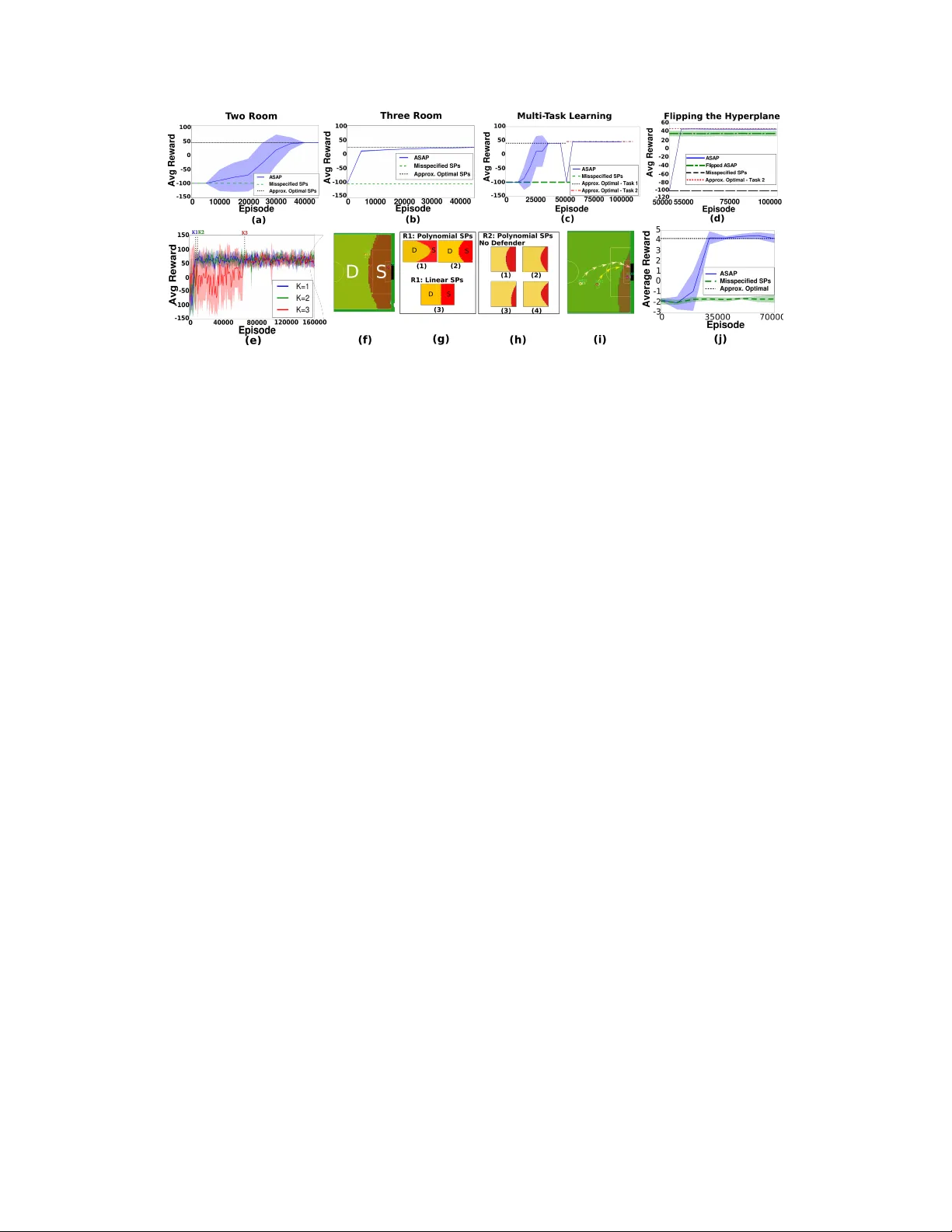
Adaptiv e Skills Adaptiv e Partitions (ASAP) Daniel J. Mank owitz Electrical Engineering Department, The T echnion - Israel Institute of T echnology , Haifa 32000, Israel danielm@tx.technion.ac.il Timoth y A. Mann Google Deepmind London, UK timothymann@google.com Shie Mannor Electrical Engineering Department, The T echnion - Israel Institute of T echnology , Haifa 32000, Israel shie@ee.technion.ac.il Abstract W e introduce the Adapti ve Skills, Adapti ve P artitions (ASAP) frame work that (1) learns skills (i.e., temporally e xtended actions or options) as well as (2) where to apply them. W e belie ve that both (1) and (2) are necessary for a truly general skill learning frame work, which is a ke y b uilding block needed to scale up to lifelong learning agents. The ASAP framew ork can also solve related new tasks simply by adapting where it applies its e xisting learned skills. W e prov e that ASAP con verges to a local optimum under natural conditions. Finally , our experimental results, which include a RoboCup domain, demonstrate the ability of ASAP to learn where to reuse skills as well as solve multiple tasks with considerably less experience than solving each task from scratch. 1 Introduction Human-decision making in volv es decomposing a task into a course of action. The course of action is typically composed of abstract, high-le vel actions that may e xecute o ver dif ferent timescales (e.g., walk to the door or make a cup of coffee). The decision-maker then chooses actions to ex ecute to solve the task. These actions may need to be r eused at different points in the task. In addition, the actions may need to be used across multiple, related tasks. Consider , for example, the task of building a city . The course of action to building a city may inv olve building the foundations, laying down se wage pipes as well as building houses and shopping malls. Each action operates o ver multiple timescales and certain actions (such as b uilding a house) may need to be reused if additional units are required. In addition, these actions can be reused if a neighboring city needs to be dev eloped (multi-task scenario). Reinforcement Learning (RL) represents actions that last for multiple timescales as T emporally Extended Actions (TEAs) (Sutton et al., 1 999), also referred to as options, skills (K onidaris & Barto, 2009) or macro-actions (Hauskrecht, 1998). It has been shown both experimentally Precup & Sutton (1997); Sutton et al. (1999); Silver & Ciosek (2012) and theoretically (Mann & Mannor, 2014) that TEAs speed up the con ver gence rates of RL planning algorithms. TEAs are seen as a potentially viable solution to making RL truly scalable. TEAs in RL have become popular in many domains including RoboCup soccer (Bai et al., 2012), video games (Mann et al., 2015) and Robotics (Fu et al., 2015). Here, decomposing the domains into temporally extended courses of action (strategies in RoboCup, strategic mov e combinations in video games and skill controllers in Robotics for example) has generated impressiv e solutions. From here on in, we will refer to TEAs as skills. T able 1: Comparison of Approaches to ASAP Automated Skill Automatic Continuous Learning Correcting Learning Skill State Reusable Model with Policy Composition Multitask Skills Misspecification Gradient Learning ASAP (this paper) X X X X X da Silva et al. 2012 X × X × × K onidaris & Barto 2009 × X × × × Bacon & Precup 2015 X × × × × Eaton & Ruvolo 2013 × × X × × Masson & K onidaris 2015 × × × × × A course of action is defined by a policy . A policy is a solution to a Markov Decision Process (MDP) and is defined as a mapping from states to a probability distribution o ver actions. That is, it tells the RL agent which action to perform gi ven the agent’ s current state. W e will refer to an inter -skill policy as being a policy that tells the agent which skill to e xecute, gi ven the current state. A truly general skill learning frame work must (1) learn skills as well as (2) automatically compose them together (as stated by Bacon & Precup (2015)) and determine where each skill should be ex ecuted (the inter -skill policy). This framew ork should also determine (3) where skills can be reused in dif ferent parts of the state space and (4) adapt to changes in the task itself. Finally it should also be able to (5) correct model misspecification (Manko witz et al., 2014). Model misspecification is defined as having an unsatisf actory set of skills and inter-skill polic y that provide a sub-optimal solution to a giv en task. This skill learning framework should be able to correct the set of misspecified skills and inter-skill polic y to obtain a near-optimal solution. A number of works ha ve addressed some of these issues separately as shown in T able 1. Howe ver , no work, to the best of our knowledge, has combined all of these elements into a truly general skill-learning framew ork. Our framew ork entitled ‘ Adaptiv e Skills, Adapti ve Partitions (ASAP)’ is the first of its kind to incorporate all of the abo ve-mentioned elements into a single framew ork, as sho wn in T able 1, and solve continuous state MDPs. It recei ves as input a misspecified model (a sub-optimal set of skills and inter -skill policy). The ASAP framework corrects the misspecification by simultaneously learning a near-optimal skill-set and inter -skill policy which are both stored, in a Bayesian-like manner , within the ASAP policy . In addition, ASAP automatically composes skills together , learns where to reuse them and learns skills across multiple tasks. Main Contributions: (1) The Adaptiv e Skills, Adapti ve Partitions (ASAP) algorithm that automati- cally corrects a misspecified model. It learns a set of near-optimal skills, automatically composes skills together and learns an inter-skill policy to solv e a giv en task. (2) Learning skills ov er multiple different tasks by automatically adapting both the inter -skill policy and the skill set. (3) ASAP can determine where skills should be reused in the state space. (4) Theoretical con ver gence guarantees. 2 Background Reinfor cement Learning Problem: A Marko v Decision Process is defined by a 5 -tuple h X, A, R, γ , P i where X is the state space, A is the action space, R ∈ [ − b, b ] is a bounded re- ward function, γ ∈ [0 , 1] is the discount factor and P : X × A → [0 , 1] X is the transition probability function for the MDP . The solution to a MDP is a policy π : X → ∆ A which is a function mapping states to a probability distribution o ver actions. An optimal policy π ∗ : X → ∆ A determines the best actions to take so as to maximize the expected reward. The value function V π ( x ) = E a ∼ π ( ·| a )  R ( x, a )  + γ E x 0 ∼ P ( ·| x,a )  V π ( x 0 )  defines the expected re ward for follo wing a policy π from state x . The optimal expected reward V π ∗ ( x ) is the expected value obtained for following the optimal polic y from state x . Policy Gradient: Policy Gradient (PG) methods hav e enjoyed success in recent years especially in the fields of robotics (Peters & Schaal, 2006, 2008). The goal in PG is to learn a policy π θ that maximizes the expected return J ( π θ ) = R τ P ( τ ) R ( τ ) dτ , where τ is a set of trajectories, P ( τ ) is the probability of a trajectory and R ( τ ) is the reward obtained for a particular trajectory . P ( τ ) is defined as P ( τ ) = P ( x 0 )Π T k =0 P ( x k +1 | x k , a k ) π θ ( a k | x k ) . Here, x k ∈ X is the state at the k th timestep of the trajectory; a k ∈ A is the action at the k th timestep; T is the trajectory length. Only the policy , in the general formulation of policy gradient, is parameterized with parameters θ . The 2 idea is then to update the policy parameters using stochastic gradient descent leading to the update rule θ t +1 = θ t + η ∇ J ( π θ ) , where θ t are the policy parameters at timestep t , ∇ J ( π θ ) is the gradient of the objectiv e function with respect to the parameters and η is the step size. 3 Skills, Skill Partitions and Intra-Skill P olicy Skills: A skill is a parameterized T emporally Extended Action (TEA) (Sutton et al., 1999). The power of a skill is that it incorporates both generalization (due to the parameterization) and temporal abstraction . Skills are a special case of options and therefore inherit many of their useful theoretical properties (Sutton et al., 1999; Precup et al., 1998). Definition 1. A Skill ζ is a TEA that consists of the two-tuple ζ = h σ θ , p i wher e σ θ : X → ∆ A is a parameterized, intra-skill policy with parameters θ ∈ R d and p : X → [0 , 1] is the termination pr obability distribution of the skill. Skill Partitions: A skill, by definition, performs a specialized task on a sub-re gion of a state space. W e refer to these sub-regions as Skill Partitions (SPs) which are necessary for skills to specialize during the learning process. A given set of SPs cov ering a state space ef fectiv ely define the inter-skill policy as they determine where each skill should be ex ecuted. These partitions are unknown a-priori and are generated using intersections of hyperplane half-spaces. Hyperplanes provide a natural w ay to automatically compose skills together . In addition, once a skill is being executed, the agent needs to select actions from the skill’ s intra-skill polic y σ θ . W e ne xt utilize SPs and the intra-skill polic y for each skill to construct the ASAP policy , defined in Section 4. W e now define a skill hyperplane. Definition 2. Skill Hyperplane (SH): Let ψ x,m ∈ R d be a vector of featur es that depend on a state x ∈ X and an MDP envir onment m . Let β i ∈ R d be a vector of hyperplane parameter s. A skill hyperplane is defined as ψ T x,m β i = L , wher e L is a constant. In this work, we interpret hyperplanes to mean that the intersection of skill hyperplane half spaces form sub-regions in the state space called Skill Partitions (SPs), defining where each skill is executed. Figure 1 a contains two example skill hyperplanes h 1 , h 2 . Skill ζ 1 is e xecuted in the SP defined by the intersection of the positi ve half-space of h 1 and the neg ativ e half-space of h 2 . The same ar gument applies for ζ 0 , ζ 2 , ζ 3 . From here on in, we will refer to skill ζ i interchangeably with its index i . Skill hyperplanes have two functions: (1) They automatically compose skills together , creating chainable skills as desired by Bacon & Precup (2015). (2) They define SPs which enable us to deriv e the probability of executing a skill, gi ven a state x and MDP m . First, we need to be able to uniquely identify a skill. W e define a binary v ector B = [ b 1 , b 2 , · · · , b K ] ∈ { 0 , 1 } K where b k is a Bernoulli random variable and K is the number of skill hyperplanes. W e define the skill index i = P K k =1 2 k − 1 b k as a sum of Bernoulli random variables b k . Note that this is but one way to generate skill partitions. In principle this setup defines 2 K skills, but in practice, far fewer skills are typically used (see experiments). Furthermore, the complexity of the SP is governed by the VC-dimension. W e can no w define the probability of e xecuting skill i as a Bernoulli likelihood in Equation 1. p ( i | x, m ) = P " i = K X k =1 2 k − 1 b k # = Y k p k ( b k = i k | x, m ) . (1) Here, i k ∈ { 0 , 1 } is the v alue of the k th bit of B , x is the current state and m is a description of the MDP . The probability p k ( b k = 1 | x, m ) and p k ( b k = 0 | x, m ) are defined in Equation 2. p k ( b k = 1 | x, m ) = 1 1 + exp( − αψ T ( x,m ) β k ) , p k ( b k = 0 | x, m ) = 1 − p k ( b k = 1 | x, m ) . (2) W e have made use of the logistic sigmoid function to ensure valid probabilities where ψ T x,m β k is a skill hyperplane and α > 0 is a temperature parameter . The intuition here is that the k th bit of a skill, b k = 1 , if the skill hyperplane ψ T x,m β k > 0 meaning that the skill’ s partition is in the positi ve half-space of the hyperplane. Similarly , b k = 0 if ψ T x,m β k < 0 corresponding to the negati ve half-space. Using skill 3 as an example with K = 2 hyperplanes in Figure 1 a , we would define the Bernoulli likelihood of ex ecuting ζ 3 as p ( i = 3 | x, m ) = p 1 ( b 1 = 1 | x, m ) · p 2 ( b 2 = 1 | x, m ) . 3 Intra-Skill Policy: Now that we can define the probability of ex ecuting a skill based on its SP , we define the intra-skill polic y σ θ for each skill. The Gibb’ s distrib ution is a commonly used function to define policies in RL (Sutton et al., 1999). Therefore we define the intra-skill policy for skill i , parameterized by θ i ∈ R d as σ θ i ( a | s ) = exp ( αφ T x,a θ i ) P b ∈ A exp ( αφ T x,b θ i ) . (3) Here, α > 0 is the temperature, φ x,a ∈ R d is a feature vector that depends on the current state x ∈ X and action a ∈ A . No w that we hav e a definition of both the probability of e xecuting a skill and an intra-skill policy , we need to incorporate these distributions into the policy gradient setting using a generalized trajectory . Generalized T rajectory: A generalized trajectory is necessary to deriv e policy gradient update rules with respect to the parameters Θ , β as will be shown in Section 4. A typical trajectory is usually defined as τ = ( x t , a t , r t , x t +1 ) T t =0 where T is the length of the trajectory . For a generalized trajectory , our algorithm emits a class i t at each timestep t ≥ 1 , which denotes the skill that was ex ecuted. The generalized trajectory is defined as g = ( x t , a t , i t , r t , x t +1 ) T t =0 . The probability of a generalized trajectory , as an extension to the PG trajectory in Section 2, is no w , P Θ ,β ( g ) = P ( x 0 ) Q T t =0 P ( x t +1 | x t , a t ) P β ( i t | x t , m ) σ θ i ( a t | x t ) , where P β ( i t | x t , m ) is the probability of a skill being ex ecuted, gi ven the state x t ∈ X and en vironment m at time t ≥ 1 ; σ θ i ( a t | x t ) is the probability of ex ecuting action a t ∈ A at time t ≥ 1 gi ven that we are e xecuting skill i . The generalized trajectory is now a function of tw o parameter vectors θ and β . 4 Adaptive Skills, Adapti ve P artitions (ASAP) Framework The Adaptive Skills, Adaptive P artitions (ASAP) framew ork simultaneously learns a near-optimal set of skills and SPs (inter -skill policy), gi ven an initially misspecified model. ASAP automatically composes skills together and allows for a multi-task setting as it incorporates the en vironment m into its hyperplane feature set. W e ha ve pre viously defined two important distributions P β ( i t | x t , m ) and σ θ i ( a t | x t ) respectiv ely . These distributions are used to collecti vely define the ASAP policy which is presented belo w . Using the notion of a generalized trajectory , the ASAP polic y can be learned in a policy gradient setting. ASAP Policy: Assume that we are giv en a probability distribution µ ov er MDPs with a d-dimensional state-action space and a z -dimensional vector describing each MDP . W e define β as a ( d + z ) × K matrix where each column β i represents a skill hyperplane, and Θ is a ( d × 2 K ) matrix where each column θ j parameterizes an intra-skill policy . Using the previously defined distributions, we now define the ASAP policy . Definition 3. (ASAP P olicy). Given K skill hyperplanes, a set of 2 K skills Σ = { ζ i | i = 1 , · · · 2 K } , a state space x ∈ X , a set of actions a ∈ A and an MDP m fr om a hypothesis space of MDPs, the ASAP policy is defined as, π Θ ,β ( a | x, m ) = 2 K X i =1 p β ( i | x, m ) σ θ i ( a | x ) , (4) wher e P β ( i | x, m ) and σ θ i ( a | s ) ar e the distributions as defined in Equations 1 and 3 r espectively . This is a powerful description for a policy , which resembles a Bayesian approach, as the policy takes into account the uncertainty of the skills that are executing as well as the actions that each skill’ s intra-skill policy chooses. W e now define the ASAP objecti ve with respect to the ASAP polic y . ASAP Objective: W e defined the policy with respect to a hypothesis space of m MDPs. W e now need to define an objective function which takes this hypothesis space into account. Since we assume that we are provided with a distribution µ : M → [0 , 1] ov er possible MDP models m ∈ M , with a d -dimensional state-action space, we can incorporate this into the ASAP objectiv e function: ρ ( π Θ ,β ) = Z µ ( m ) J ( m ) ( π Θ ,β ) dm , (5) 4 where π Θ ,β is the ASAP polic y and J ( m ) ( π Θ ,β ) is the expected return for MDP m with respect to the ASAP policy . T o simplify the notation, we group all of the parameters into a single parameter vector Ω = [ vec (Θ) , v ec ( β )] . W e define the expected reward for generalized trajectories g as J ( π Ω ) = R g P Ω ( g ) R ( g ) dg , where R ( g ) is rew ard obtained for a particular trajectory g . This is a slight v ariation of the original policy gradient objecti ve defined in Section 2. W e then insert J ( π Ω ) into Equation 5 and we get the ASAP objectiv e function ρ ( π Ω ) = Z µ ( m ) J ( m ) ( π Ω ) dm , (6) where J ( m ) ( π Ω ) is the expected return for policy π Ω in MDP m . Next, we need to deri ve gradient update rules to learn the parameters of the optimal policy π ∗ Ω that maximizes this objectiv e. ASAP Gradients: T o learn both intra-skill policy parameters matrix Θ as well as the hyperplane parameters matrix β (and therefore implicitly the SPs), we deriv e an update rule for the policy gradient frame work with generalized trajectories. The deriv ation is in the supplementary material. The first step in volves calculating the gradient of the ASAP objecti ve function yielding the ASAP gradient (Theorem 1). Theorem 1. (ASAP Gradient Theor em). Suppose that the ASAP objective function is ρ ( π Ω ) = R µ ( m ) J ( m ) ( π Ω ) dm wher e µ ( m ) is a distribution over MDPs m and J ( m ) ( π Ω ) is the expected r eturn for MDP m whilst following policy π Ω , then the gradient of this objective is: ∇ Ω ρ ( π Ω ) = E µ ( m )  E P ( m ) Ω ( g )  H ( m ) X i =0 ∇ Ω Z ( m ) Ω ( x t , i t , a t ) R ( m )  , wher e Z ( m ) Ω ( x t , i t , a t ) = log P β ( i t | x t , m ) σ θ i ( a t | x t ) , H ( m ) is the length of a trajectory for MDP m ; R ( m ) = P H ( m ) i =0 γ i r i is the discounted cumulative r ewar d for trajectory H ( m ) 1 . If we are able to derive ∇ Ω Z ( m ) Ω ( x t , i t , a t ) , then we can estimate the gradient ∇ Ω ρ ( π Ω ) . W e will refer to Z ( m ) Ω = Z ( m ) Ω ( x t , i t , a t ) where it is clear from conte xt. It turns out that it is possible to deri ve this term as a result of the generalized trajectory . This yields the gradients ∇ Θ Z ( m ) Ω and ∇ β Z ( m ) Ω in Theorems 2 and 3 respectiv ely . The deri vations can be found the supplementary material. Theorem 2. ( Θ Gradient Theor em). Suppose that Θ is a ( d × 2 K ) matrix where each column θ j parameterizes an intra-skill policy . Then the gradient ∇ θ i t Z ( m ) Ω corr esponding to the intra-skill parameters of the i th skill at time t is: ∇ θ i t Z ( m ) Ω = αφ x t ,a t − α  P b ∈ A φ x t ,b t exp( αφ T x t ,b t Θ i t )   P b ∈ A exp( αφ T x t ,b t Θ i t )  , wher e α > 0 is the temperatur e parameter and φ x t ,a t ∈ R d × 2 K is a feature vector of the curr ent state x t ∈ X t and the curr ent action a t ∈ A t . Theorem 3. ( β Gradient Theor em). Suppose that β is a ( d + z ) × K matrix wher e each column β k r epr esents a skill hyperplane . Then the gr adient ∇ β k Z ( m ) Ω corr esponding to parameter s of the k th hyperplane is: ∇ β k, 1 Z ( m ) Ω = αψ ( x t ,m ) exp( − αψ T x t ,m β k )  1 + exp( − αψ T x t ,m β k )  , ∇ β k, 0 Z ( m ) Ω = − αψ x t ,m + αψ x t ,m exp( − αψ T x t ,m β k )  1 + exp( − αψ T x t ,m β k )  (7) wher e α > 0 is the hyperplane temperatur e parameter , ψ T ( x t ,m ) β k is the k th skill hyperplane for MDP m , β k, 1 corr esponds to locations in the binary vector equal to 1 ( b k = 1 ) and β k, 0 corr esponds to locations in the binary vector equal to 0 ( b k = 0 ). Using these gradient updates, we can then order all of the gradients into a vector ∇ Ω Z ( m ) Ω = h∇ θ 1 Z ( m ) Ω . . . ∇ θ 2 k Z ( m ) Ω , ∇ β 1 Z ( m ) Ω . . . ∇ β k Z ( m ) Ω i and update both the intra-skill policy parameters and hyperplane parameters for the given task (learning a skill set and SPs). Note that the updates occur on a single time scale. This is formally stated in the ASAP Algorithm. 1 These expectations can easily be sampled (see supplementary material). 5 5 ASAP Algorithm W e present the ASAP algorithm (Algorithm 1) that dynamically and simultaneously learns skills, the inter-skill polic y and automatically composes skills together by learning SPs. The skills ( Θ matrix) and SPs ( β matrix) are initially arbitrary and therefore form a misspecified model . Line 2 combines the skill and hyperplane parameters into a single parameter vector Ω . Lines 3 − 7 learns the skill and hyperplane parameters (and therefore implicitly the skill partitions). In line 4 a generalized trajectory is generated using the current ASAP policy . The gradient ∇ Ω ρ ( π Ω ) is then estimated in line 5 from this trajectory and updates the parameters in line 6 . This is repeated until the skill and hyperplane parameters hav e con ver ged, thus correcting the misspecified model. Theorem 4 provides a con ver gence guarantee of ASAP to a local optimum (see supplementary material for the proof). Algorithm 1 ASAP Require: φ s,a ∈ R d {state-action feature vector}, ψ x,m ∈ R ( d + z ) {skill hyperplane feature v ector}, K {The number of hyperplanes}, Θ ∈ R d × 2 K {An arbitrary skill matrix}, β ∈ R ( d + z ) × K {An arbitrary skill hyperplane matrix}, µ ( m ) {A distribution o ver MDP tasks} 1: Z = ( | d || 2 K | + | ( d + z ) K | ) {Define the number of parameters} 2: Ω = [ vec (Θ) , vec ( β )] ∈ R Z 3: r epeat 4: Perform a trial (which may consist of multiple MDP tasks) and obtain x 0: H , i 0: H , a 0: H , r 0: H , m 0: H {states, skills, actions, rew ards, task-specific information} 5: ∇ Ω ρ ( π Ω ) =  P m  P T ( m ) i =0 ∇ Ω Z ( m ) (Ω) R ( m )  { T is the task episode length} 6: Ω → Ω + η ∇ Ω ρ ( π Ω ) 7: until parameters Ω hav e con ver ged 8: r eturn Ω Theorem 4. Con ver gence of ASAP: Given an ASAP policy π (Ω) , an ASAP objective over MDP models ρ ( π Ω ) as well as the ASAP gradient update rules. If (1) the step-size η k satisfies lim k →∞ η k = 0 and P k η k = ∞ ; (2) The second derivative of the policy is bounded and we have bounded r ewar ds. Then, the sequence { ρ ( π Ω ,k ) } ∞ k =0 con ver ges suc h that lim k →∞ ∂ ρ ( π Ω ,k ) ∂ Ω = 0 almost sur ely . 6 Experiments The experiments ha ve been performed on four dif ferent continuous domains: the T wo Rooms (2R) domain (Figure 1 b ), the Flipped 2R domain (Figure 1 c ), the Three r ooms (3R) domain (Figure 1 d ) and RoboCup domains (Figure 1 e ) that include a one-on-one scenario between a striker and a goalkeeper (R1), a two-on-one scenario of a striker against a goalkeeper and a defender (R2), and a striker against two defenders and a goalkeeper (R3) (see supplementary material). In each experiment, ASAP is provided with a misspecified model ; that is, a set of skills and SPs (the inter-skill policy) that achie ve degenerate, sub-optimal performance. ASAP corrects this misspecified model in each case to learn a set of near -optimal skills and SPs. For each experiment we implement ASAP using Actor -Critic Policy Gradient (A C-PG) as the learning algorithm 2 . The T wo-Room and Flipped Room Domains (2R): In both domains, the agent (red ball) needs to reach the goal location (blue square) in the shortest amount of time. The agent receiv es constant negati ves rewards and upon reaching the goal, receives a large positi ve rew ard. There is a wall dividing the en vironment which creates two rooms. The state space is a 4 -tuple consisting of the continuous h x ag ent , y ag ent i location of the agent and the h x g oal , y g oal i location of the center of the goal. The agent can mov e in each of the four cardinal directions. For each e xperiment in volving the two room domains, a single hyperplane is learned (resulting in tw o SPs) with a linear feature vector representation ψ x,m = [1 , x ag ent , y ag ent ] . In addition, a skill is learned in each of the two SPs. The intra-skill policies are represented as a probability distribution o ver actions. A utomated Hyperplane and Skill Learning : Using ASAP , the agent learned intuiti ve SPs and skills as seen in Figure 1 f and g . Each colored region corresponds to a SP . The white arrows hav e been 2 A C-PG works well in practice and can be tri vially incorporated into ASAP with con ver gence guarantees 6 Figure 1: ( a ) The intersection of skill hyperplanes { h 1 , h 2 } form four partitions, each of which defines a skill’ s execution re gion (the inter -skill policy). The ( b ) 2R, ( c ) Flipped 2R, ( d ) 3R and ( e ) RoboCup domains (with a v arying number of defenders for R1,R2,R3). The learned skills and Skill Partitions (SPs) for the ( f ) 2R, ( g ) Flipped 2R, ( h ) 3R and ( i ) across multiple tasks. superimposed onto the figures to indicate the skills learned for each SP . Since each intra-skill policy is a probability distrib ution o ver actions, each skill is unable to solv e the entire task on its o wn. ASAP has taken this into account and has positioned the hyperplane accordingly such that the gi ven skill representation can solve the task. Figure 2 a shows that ASAP impro ves upon the initial misspecified partitioning to attain near-optimal performance compared to executing ASAP on the fixed initial misspecified partitioning and on a fixed approximately optimal partitioning. Multiple Hyperplanes: W e analyzed the ASAP framework when learning multiple hyperplanes in the two room domain. As seen in Figure 2 e , increasing the number of hyperplanes K , does not hav e an impact on the final solution in terms of average re ward. Ho wev er , it does increase the computational complexity of the algorithm since 2 K skills need to be learned. The approximate points of con ver gence are marked in the figure as K 1 , K 2 and K 3 , respectively . In addition, two skills dominate in each case producing similar partitions to those seen in Figure 1 a (see supplementary material) indicating that ASAP learns that not all skills are necessary to solve the task. Multitask Learning : W e first applied ASAP to the 2R domain (T ask 1) and attained a near optimal av erage re ward (Figure 2 c ). It took approximately 35000 episodes to get near -optimal performance and resulted in the SPs and skill set sho wn in Figure 1 i (top). Using the learned SPs and skills, ASAP was then able to adapt and learn a new set of SPs and skills to solve a diff erent task (Flipped 2R - T ask 2) in only 5000 episodes (Figure 2 c ) indicating that the parameters learned from the old task provided a good initialization for the ne w task. The knowledge transfer is seen in Figure 1 i (bottom) as the SPs do not significantly change between tasks, yet the skills are completely relearned. W e also wanted to see whether we could flip the SPs; that is, switch the sign of the hyperplane parameters learned in the 2R domain and see whether ASAP can solve the Flipped 2R domain (T ask 2) without any additional learning. Due to the symmetry of the domains, ASAP was indeed able to solve the ne w domain and attained near-optimal performance (Figure 2 d ). This is an exciting result as many problems, especially na vigation tasks, possess symmetrical characteristics. This insight could dramatically reduce the sample complexity of these problems. The Three-Room Domain (3R): The 3R domain (Figure 1 d ), is similar to the 2R domain reg arding the goal, state-space, available actions and rew ards. Howe ver , in this case, there are two walls, dividing the state space into three rooms. The hyperplane feature vector ψ x,m consists of a single fourier feature. The intra-skill policy is a probability distribution o ver actions. The resulting learned hyperplane partitioning and skill set are shown in Figure 1 h . Using this partitioning ASAP achiev ed near optimal performance (Figure 2 b ). This e xperiment shows an insightful and unexpected result. Reusable Skills : Using this hyperplane representation, ASAP was able to not only learn the intra-skill policies and SPs, b ut also that skill ‘ A ’ needed to be r eused in two dif ferent parts of the state space (Figure 1 h ). ASAP therefore sho ws the potential to automatically create reusable skills. RoboCup Domain: The RoboCup 2D soccer simulation domain (Akiyama & Nakashima, 2014) is a 2D soccer field (Figure 1 e ) with two opposing teams. W e utilized three RoboCup sub-domains 3 R1, R2 and R3 as mentioned previously . In these sub-domains, a striker (the agent) needs to learn to dribble the ball and try and score goals past the goalkeeper . State space: R1 domain - the continuous locations of the striker h x strik er , y strik er i , the ball h x ball , y ball i , the goalkeeper h x g oalkeeper , y g oalkeeper i and the constant goal location h x g oal , y g oal i . R2 domain - we hav e the addition of the defender’ s location h x def ender , y def ender i to the state space. R3 domain - we add the locations of two defenders. Featur es: For the R1 domain, we tested both a linear and degree two 3 https://github .com/mhauskn/HFO.git 7 Figure 2: A verage rew ard of the learned ASAP policy compared to the approximately optimal SPs and skill set as well as the initial misspecified model. This is for the ( a ) 2R, ( b ) 3R, ( c ) 2R learning across multiple tasks and the ( d ) 2R without learning by flipping the hyperplane. ( e ) The average rew ard of the learned ASAP policy for a varying number of K hyperplanes. ( f ) The learned SPs and skill set for the R1 domain. ( g ) The learned SPs using a polynomial hyperplane ( 1 ),( 2 ) and linear hyperplane ( 3 ) representation. ( h ) The learned SPs using a polynomial hyperplane representation without the defender’ s location as a feature ( 1 ) and with the defender’ s x location ( 2 ), y location ( 3 ), and h x, y i location as a feature ( 4 ). ( i ) The dribbling behavior of the striker when taking the defender’ s y location into account. ( j ) The average re ward for the R1 domain. polynomial feature representation for the hyperplanes. For the R2 and R3 domains, we also utilized a degree two polynomial hyperplane feature representation. Actions: The striker has three actions which are ( 1 ) mov e to the ball ( M ), ( 2 ) mov e to the ball and dribble to wards the goal ( D ) ( 3 ) mov e to the ball and shoot towards the goal ( S ). Rewards: The reward setup is consistent with logical football strate gies (Hausknecht & Stone, 2015; Bai et al., 2012). Small ne gativ e (positi ve) rewards for shooting from outside (inside) the box and dribbling when inside (outside) the box. Large negati ve rew ards for losing possession and kicking the ball out of bounds. Large positi ve rew ard for scoring. Different SP Optimas : Since ASAP attains a locally optimal solution, it may sometimes learn different SPs. For the polynomial hyperplane feature representation, ASAP attained two dif ferent solutions as shown in Figure 2 g (1) as well as Figures 2 f , 2 g (2) , respectively . Both achieve near optimal performance compared to the approximately optimal scoring controller (see supplementary material). For the linear feature representation, the SPs and skill set in Figure 2 g (3) is obtained and achiev ed near -optimal performance (Figure 2 j ), outperforming the polynomial representation. SP Sensitivity : In the R2 domain, an additional player (the defender) is added to the game. It is expected that the presence of the defender will af fect the shape of the learned SPs. ASAP again learns intuitiv e SPs. Howe ver , the shape of the learned SPs change based on the pre-defined hyperplane feature vector ψ m,x . Figure 2 h (1) shows the learned SPs when the location of the defender is not used as a hyperplane feature. When the x location of the defender is utilized, the ‘flatter’ SPs are learned in Figure 2 h ( 2 ). Using the y location of the defender as a hyperplane feature causes the hyperplane offset sho wn in Figure 2 h ( 3 ). This is due to the striker learning to dribble around the defender in order to score a goal as seen in Figure 2 i . Finally , taking the h x, y i location of the defender into account results in the ‘squashed’ SPs sho wn in Figure 2 h ( 4 ) clearly showing the sensitivity and adaptability of ASAP to dynamic factors in the en vironment. 7 Discussion W e hav e presented the Adaptiv e Skills, Adaptiv e Partitions (ASAP) framew ork that is able to automatically compose skills together and learns a near-optimal skill set and skill partitions (the inter-skill polic y) simultaneously to correct an initially misspecified model. W e deriv ed the gradient update rules for both skill and skill hyperplane parameters and incorporated them into a policy gradient framework. This is possible due to our definition of a generalized trajectory . In addition, ASAP has shown the potential to learn across multiple tasks as well as automatically reuse skills. These are the necessary requirements for a truly general skill learning framework and can be applied to lifelong learning problems (Ammar et al., 2015; Thrun & Mitchell, 1995). An exciting e xtension of this w ork is to incorporate it into a Deep Reinforcement Learning frame work, where both the skills and ASAP policy can be represented as deep networks. 8 References Akiyama, Hidehisa and Nakashima, T omoharu. Helios base: An open source package for the robocup soccer 2d simulation. In RoboCup 2013: Robot W orld Cup XVII , pp. 528–535. Springer , 2014. Ammar , Haitham Bou, T utunov , Rasul, and Eaton, Eric. Safe policy search for lifelong reinforcement learning with sublinear regret. arXiv pr eprint arXiv:1505.05798 , 2015. Bacon, Pierre-Luc and Precup, Doina. The option-critic architecture. In NIPS Deep Reinforcement Learning W orkshop , 2015. Bai, Aijun, W u, Feng, and Chen, Xiaoping. Online planning for large mdps with maxq decomposition. In AAMAS , 2012. da Silva, B.C., K onidaris, G.D., and Barto, A.G. Learning parameterized skills. In ICML , 2012. Eaton, Eric and Ruvolo, P aul L. Ella: An efficient lifelong learning algorithm. In Pr oceedings of the 30th international confer ence on machine learning (ICML-13) , pp. 507–515, 2013. Fu, Justin, Levine, Ser gey , and Abbeel, Pieter . One-shot learning of manipulation skills with online dynamics adaptation and neural network priors. arXiv pr eprint arXiv:1509.06841 , 2015. Hausknecht, Matthe w and Stone, Peter . Deep reinforcement learning in parameterized action space. arXiv pr eprint arXiv:1511.04143 , 2015. Hauskrecht, Milos, Meuleau Nicolas et. al. Hierarchical solution of markov decision processes using macro-actions. In UAI , pp. 220–229, 1998. K onidaris, George and Barto, Andrew G. Skill discovery in continuous reinforcement learning domains using skill chaining. In NIPS , 2009. Manko witz, Daniel J, Mann, T imothy A, and Mannor , Shie. T ime regularized interrupting options. Internation Confer ence on Machine Learning , 2014. Mann, T imothy A and Mannor, Shie. Scaling up approximate value iteration with options: Better policies with fe wer iterations. In Pr oceedings of the 31 st International Confer ence on Mac hine Learning , 2014. Mann, T imothy Arthur , Mankowitz, Daniel J, and Mannor , Shie. Learning when to switch between skills in a high dimensional domain. In AAAI W orkshop , 2015. Masson, W arwick and K onidaris, George. Reinforcement learning with parameterized actions. arXiv pr eprint arXiv:1509.01644 , 2015. Peters, Jan and Schaal, Stefan. Policy gradient methods for robotics. In Intelligent Robots and Systems, 2006 IEEE/RSJ International Confer ence on , pp. 2219–2225. IEEE, 2006. Peters, Jan and Schaal, Stefan. Reinforcement learning of motor skills with policy gradients. Neural Networks , 21:682–691, 2008. Precup, Doina and Sutton, Richard S. Multi-time models for temporally abstract planning. In Advances in Neural Information Pr ocessing Systems 10 (Pr oceedings of NIPS’97) , 1997. Precup, Doina, Sutton, Richard S, and Singh, Satinder . Theoretical results on reinforcement learning with temporally abstract options. In Machine Learning: ECML-98 , pp. 382–393. Springer , 1998. Silver , David and Ciosek, Kamil. Compositional Planning Using Optimal Option Models. In Pr oceedings of the 29th International Conference on Mac hine Learning , Edinbur gh, 2012. Sutton, Richard S, Precup, Doina, and Singh, Satinder . Between MDPs and semi-MDPs: A framew ork for temporal abstraction in reinforcement learning. Artificial Intelligence , 1999. Sutton, Richard S, McAllester , David, Singh, Satindar , and Mansour , Y ishay . Policy gradient methods for reinforcement learning with function approximation. In NIPS , pp. 1057–1063, 2000. Thrun, Sebastian and Mitchell, T om M. Lifelong r obot learning . Springer, 1995. 9