Scalable Algorithms for Tractable Schatten Quasi-Norm Minimization

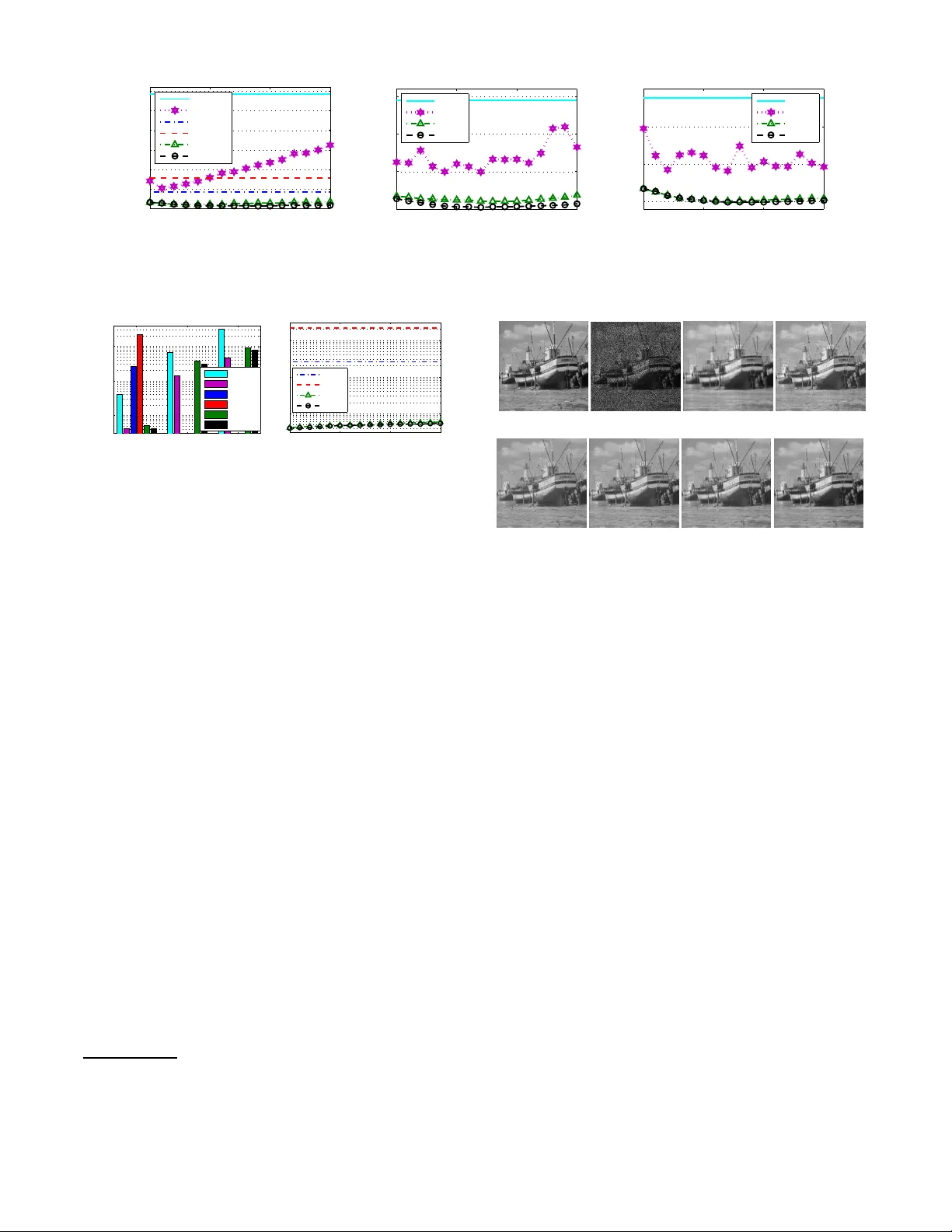
Scalable Algorithms f or T ractable Schatten Quasi-Norm Minimization Fanh ua Shang, Y uanyuan Liu, James Ch eng Departmen t of C om puter Science and Engineering , The Chinese Univ ersity of Hong K ong { fhshan g, yyliu, jcheng } @cse.cuhk.ed u.hk Abstract The Schatten- p quasi-norm (0 < p < 1 ) is usually used to re- place the standard nuclear norm i n order to approximate t he rank function more accurately . Howe ver , existing Schatten- p quasi-no rm minimization algorithms in volve sing ular value decomposition (SVD) or e igen value deco mposition (EVD) in each iteration, and thus may become very slow and impracti- cal for lar ge-scale problems. In this paper , we first define two tractable Schatten quasi-norms, i.e., the Frobenius/nuc lear hybrid and bi-nuclear quasi-norms, and then prov e that t hey are in essence the S chatten- 2 / 3 and 1 / 2 quasi-norms, re- specti vely , which lead to t he design of very efficient algo- rithms that only need to update two much smaller factor ma- trices. W e also design two efficient proximal alt ernating lin- earized minimization algorithms for solving representati ve matrix completion problems. Finally , we provide the globa l con ver gence and performance guarantees for our algorithms, which have better con vergence properties than existing algo- rithms. Experimental resu lts on synthetic and real-world data sho w that our algorithms are more accurate than the state-of- the-art methods, and are orders of magnitude faster . Intr oduction In recent years, the matrix rank minimization problem arises in a wide range of application s such as matrix completion , ro bust prin cipal compon ent analysis, low-rank representatio n, multiv ariate regression an d mu lti-task learning. T o solve such problems, Fazel, Hindi, and Boyd; Cand ` es and T ao; Recht, Fazel, and P arrilo (200 1 ; 2010; 2010) have suggested to relax the rank function by its conv ex envelope, i.e., the n uclear norm. In fact, th e nuclear norm is equiv alent to th e ℓ 1 -norm on sin gular values of a matrix, and thus it promotes a low-rank solution. Howe ver , it has been shown in (Fan and Li 2001) that the ℓ 1 -norm regularization over -pen alizes large e ntries of vectors, and results in a biased solutio n. By realizin g the intimate r elationship between them, the n uclear norm penalty also over-penalizes large sing ular values, that is, it may make the solution deviate from the original solution as the ℓ 1 -norm does (Nie , Huang, and Ding 2012; Lu et al. 2015). Com pared with the nu clear norm , the Schatten- p quasi-norm fo r 0 < p < 1 makes a closer Copyrigh t c  2016, Association for the Advan cement of Art ificial Intelligence (www .aaai.org). All rights reserved. approx imation to the rank fun ction. Consequ ently , the Schatten- p q uasi-nor m minimizatio n has attracted a great deal of attention in images recovery ( Lu and Zhang 2014; Lu et al. 2014), collaborative filtering (Nie et al. 2012; Lu et al. 2015; Mohan and Fazel 2012) and MRI anal- ysis (Majumda r and W ard 20 11). In add ition, many non-co n vex sur rogate f unction s of the ℓ 0 -norm listed in (Lu et al. 2014; Lu et al. 20 15) have been ex- tended to appro ximate the ran k function , such as SCAD (Fan and Li 200 1) and MCP (Zhang 2010). All non -conve x surrogate function s mentioned ab ove for low-rank minim ization lea d to some non-c onv ex, non- smooth, e ven non-L ipschitz optim ization problem s. Ther e- fore, it is cr ucial to dev elop fast and scalable algo rithms which are specialized to solve some alternative formula- tions. So far , Lai, Xu , and Y in (2013) pro posed an iterati ve reweighted lease squ ares ( IRucLq) a lgorithm to appro xi- mate the Sch atten- p quasi-nor m minimization prob lem, and proved that the limit point o f any conver gen t subseq uence generated by th eir algorith m is a cr itical poin t. Moreover, Lu et al. (2014) propo sed an iter ativ ely reweighted n uclear norm (I RNN) algorithm to solve many non-co n vex surrogate minimization problems. For matrix completio n pro blems, the Schatten- p quasi-no rm h as been shown to be emp irically superior to the n uclear norm (Marjanovic and Solo 2012). In addition, Zh ang, Huang, and Zhang (2013) theoretically proved that the Schatten- p quasi-nor m minimization with small p require s significantly fe wer measurements th an th e conv ex n uclear norm min imization. Howe ver, all existing algorithm s hav e to b e solved iterativ ely and inv olve SVD or EVD in eac h iter ation, which incurs hig h comp utational cost and is too expensive for solving large-scale pro b- lems (Cai and Osher 2013; Liu et al. 2014). In co ntrast, as an alternative non-conve x formula- tion of the nu clear nor m, the b ilinear spectral reg- ularization as in (Srebro , Rennie, and Jaakkola 2004; Recht, Fazel, and Parrilo 2010) has bee n successfully ap- plied in m any large-scale application s, e.g., collabo rative filtering (Mitra, Sheorey , an d Chellappa 2010). As th e Schatten- p quasi-no rm is equivalent to the ℓ p quasi-nor m on singular values of a matrix, it is n atural to ask th e following question: can we design equiva lent matrix factorization forms for the cases of the Schatten quasi-n orm, e.g., p = 2 / 3 or 1 / 2 ? In order to an swer the above question, in th is paper we first define tw o tractable Schatten quasi-norms, i.e., the Frobeniu s/nuclear hybr id and bi-nuclear q uasi-nor ms. W e then prove that they ar e in essence the Schatten- 2 / 3 and 1 / 2 quasi-nor ms, respectively , for solvin g who se m inimization we o nly n eed to per form SVDs on two much smaller fac- tor matrices as co ntrary to th e larger ones used in existing algorithm s, e.g., I RNN. Therefore , o ur method is par ticu- larly u seful fo r many “b ig da ta” app lications that n eed to deal with la rge, hig h d imensional d ata with missing values. T o the best o f ou r knowledge, this is the first p aper to scale Schatten quasi-no rm solvers to the Netflix dataset. More- over , we provide th e global co n vergence and recovery per- forman ce gu arantees f or our algorithm s. I n other w or ds, this is the best gu aranteed con vergence f or algorithm s that solve such challengin g problem s. Notations and Backgr ound The Schatten - p norm ( 0 < p < ∞ ) of a m atrix X ∈ R m × n ( m ≥ n ) is de fined as k X k S p , n X i =1 σ p i ( X ) ! 1 /p , where σ i ( X ) den otes the i -th singu lar value of X . When p = 1 , the Schatten- 1 no rm is the we ll-known n u- clear no rm, k X k ∗ . I n add ition, as the non-c onv ex sur- rogate for the rank function, th e Schatten- p qu asi-norm with 0 < p < 1 is a better appr oximation than the nuclear norm (Zhang , Huang, and Zhang 201 3) (anal- ogous to the super iority of the ℓ p quasi-nor m to the ℓ 1 - norm (Daubech ies et a l. 2010)). T o recover a low-rank matrix from some lin ear observa- tions b ∈ R s , we con sider the following general Sch atten- p quasi-nor m minimization problem, min X λ k X k p S p + f ( A ( X ) − b ) , (1) where A : R m × n → R s denotes th e linear measure- ment operator, λ > 0 is a r egularization para meter, an d the loss function f ( · ) : R s → R g enerally den otes certain measure ment for characterizing A ( X ) − b . The above formulation can a ddress a wide range of prob lems, such as matrix completion (Marjanovic and Solo 2012; Rohde and Tsybakov 2011) ( A is the samp ling op era- tor and f ( · ) = k · k 2 2 ), robust prin cipal compo nent analysis (Cand ` es et al. 2011; W ang, Liu, and Zh ang 2013; Shang et al. 2014) ( A is the identity opera tor and f ( · ) = k · k 1 ), and mu ltiv ariate regression ( Hsieh and Olsen 2014) ( A ( X ) = AX with A being a g iv en m atrix, an d f ( · ) = k · k 2 F ). Furthermo re, f ( · ) m ay be also ch osen as the Hinge loss in (Sreb ro, Rennie, and Jaakkola 2004) or the ℓ p quasi-nor m in (Nie et al. 2012). Analogou s to the ℓ p quasi-nor m, the Schatten- p quasi- norm is also no n-conve x for p < 1 , and its m inimization is g enerally NP- hard (L ai, Xu, and Y in 201 3). Theref ore, it is cru cial to develop ef ficient algo rithms to solve some al- ternative formulatio ns o f Schatten- p quasi-norm minim iza- tion (1). So far , o nly f ew algo rithms (Lai, Xu, and Y in 2013; Mohan and Fazel 2012; Nie et al. 201 2; Lu et al. 2014) have been d eveloped to solve such prob lems. Fu rthermo re, since all existing Scha tten- p quasi-nor m minimization algo rithms in volve SVD or EVD in each iteration , they suffer fro m a high computationa l co st o f O ( n 2 m ) , which se verely lim its their applicab ility to large-scale pro blems. Although there have b een many efforts to wards fast SVD or EVD compu- tation such as partial SVD (L arsen 2005), the performan ce of tho se m ethods is still unsatisfactory for r eal-life applica- tions (Cai and Osher 2013). T ractable Schatten Quasi-Norms As in (Srebro , Rennie, and Jaakkola 2004), the nuclear norm has the following a lternative n on-co n vex form ulations. Lemma 1. Given a matrix X ∈ R m × n with rank ( X ) = r ≤ d , the following holds: k X k ∗ = min U ∈ R m × d ,V ∈ R n × d : X = U V T k U k F k V k F = min U,V : X = U V T k U k 2 F + k V k 2 F 2 . Fro benius/Nuclear Hybrid Quasi-Norm Motiv ated by the equ iv alence relatio n b etween the nuclear norm and the bilinear spectral regularization (please refer to (Srebro, Rennie, and Jaakkola 2004; Recht, Fazel, and Parrilo 2010)), we define a Frobe - nius/nuclear hybrid (F/N) norm as follows Definition 1. F o r any matrix X ∈ R m × n with rank ( X ) = r ≤ d , we can factorize it in to two mu ch smaller matrices U ∈ R m × d and V ∈ R n × d such that X = U V T . Then the F r oben ius/nuclear hybrid norm of X is defined as k X k F/N := min X = U V T k U k ∗ k V k F . In fact, the Frobenius/n uclear hyb rid n orm is not a real norm, because it is non -conve x an d does not satisfy the triangle inequ ality of a norm. Similar to the well-k nown Schatten- p quasi-norm ( 0 < p < 1 ), the Froben ius/nuclear hybrid norm is also a quasi-nor m, and their relationship is stated in the following th eorem. Theorem 1 . The F r oben ius/nuclear hybrid n orm k·k F/N is a quasi-no rm. Su rprisingly , it is also the Schatten- 2 / 3 quasi- norm, i.e., k X k F/N = k X k S 2 / 3 , wher e k X k S 2 / 3 denotes the Schatten- 2 / 3 qua si-norm of X . Property 1. F o r any matrix X ∈ R m × n with rank ( X ) = r ≤ d , the following holds: k X k F/N = min U ∈ R m × d ,V ∈ R n × d : X = U V T k U k ∗ k V k F = min X = U V T  2 k U k ∗ + k V k 2 F 3  3 / 2 . The p roofs o f Pro perty 1 an d Th eorem 1 can be found in the Supplemen tary Mate rials. Bi-Nuclear Quasi-Norm Similar to the definition o f th e ab ove Frobenius/nu clear hy- brid norm, our bi-nuclear (BiN) no rm is na turally defined as follows. Definition 2. F or any matrix X ∈ R m × n with rank ( X ) = r ≤ d , we can factorize it in to two much smaller matrices U ∈ R m × d and V ∈ R n × d such that X = U V T . Th en the bi-nuclea r norm of X is defined as k X k BiN := min X = U V T k U k ∗ k V k ∗ . Similar to the Frobenius/nuclear hybrid norm, the b i- nuclear norm is also a q uasi-norm , as stated i n the following theorem. Theorem 2. The bi-nuclear no rm k· k BiN is a quasi-no rm. In addition , it is also the Schatten- 1 / 2 qua si-norm, i.e., k X k BiN = k X k S 1 / 2 . The pro of of Theor em 2 can be found in the Supple- mentary Materials. Due to the r elationship between the bi- nuclear quasi-norm and the Schatten- 1 / 2 qu asi-norm, it is easy to verify that the b i-nuclear quasi-nor m p ossesses the following properties. Property 2 . F or any matrix X ∈ R m × n with rank ( X ) = r ≤ d , the following hold s: k X k BiN = min X = U V T k U k ∗ k V k ∗ = min X = U V T k U k 2 ∗ + k V k 2 ∗ 2 = min X = U V T  k U k ∗ + k V k ∗ 2  2 . The following r elationship between the nuclear norm and the Frob enius nor m is well known: k X k F ≤ k X k ∗ ≤ √ r k X k F . Similarly , the analogous bo unds hold for the Frobeniu s/nuclear hybrid and b i-nuclear q uasi-nor ms, as stated in the following property . Property 3 . F or any matrix X ∈ R m × n with r ank ( X ) = r , the following inequa lities hold: k X k ∗ ≤ k X k F/N ≤ √ r k X k ∗ , k X k ∗ ≤ k X k F/N ≤k X k BiN ≤ r k X k ∗ . The pro of o f Property 3 can b e foun d in the Supplemen - tary Materials. It is easy to s ee that Prop erty 3 in turn implies that any low Frobeniu s/nuclear hybrid or bi- nuclear norm approx imation is also a low nuclear norm appr oximation . Optimization Algorithms Pro blem Formulations T o boun d th e Schatten- 2 / 3 or - 1 / 2 qu asi-norm of X by 1 3 (2 k U k ∗ + k V k 2 F ) or 1 2 ( k U k ∗ + k V k ∗ ) , we mainly consider the following g eneral structured matrix factorization formu - lation as in (Haeffele, Y oung , and V idal 20 14), min U,V λϕ ( U, V ) + f ( A ( U V T ) − b ) , (2) where the regularization term ϕ ( U, V ) denotes 1 3 (2 k U k ∗ + k V k 2 F ) or 1 2 ( k U k ∗ + k V k ∗ ) . As mentio ned above, there ar e many Schatten- p qua si- norm minimization problems for various r eal-world ap pli- cations. Therefo re, we prop ose two efficient algorith ms to solve t he fo llowing low-rank matrix completion problems: min U,V λ (2 k U k ∗ + k V k 2 F ) 3 + 1 2 kP Ω ( U V T ) − P Ω ( D ) k 2 F , (3) min U,V λ ( k U k ∗ + k V k ∗ ) 2 + 1 2 kP Ω ( U V T ) − P Ω ( D ) k 2 F , (4) where P Ω denotes the linear pro jection operato r , i.e. , P Ω ( D ) ij = D ij if ( i, j ) ∈ Ω , and P Ω ( D ) ij =0 otherwise. Due to the op erator P Ω in (3) and (4 ), we usually ne ed to intr o- duce some a uxiliary v ariables for so lving them. T o a void in- troducin g auxiliary variables, motiv ated by the prox imal al- ternating line arized minimiz ation (P ALM) method pro posed in (Bolte, Sabach, and T ebou lle 2014), we pro pose two fast P ALM algorithm s to ef ficiently solve (3) and (4). The space limitation refr ains us from fully d escribing each algorithm, but we try to give enoug h details of a representative algo- rithm for solving (3) and discussing their differences. Updating U k +1 and V k +1 with Linearizatio n T echniques Let g k ( U ) := kP Ω ( U V T k ) − P Ω ( D ) k 2 F / 2 , and then its gr a- dient is Lipschitz continu ous with constant l g k +1 , meaning that k∇ g k ( U 1 ) − ∇ g k ( U 2 ) k F ≤ l g k +1 k U 1 − U 2 k F for any U 1 , U 2 ∈ R m × d . By lin earizing g k ( U ) at U k and ad ding a proxim al ter m, then we hav e the following appro ximation: b g k ( U, U k ) = g k ( U k ) + h∇ g k ( U k ) , U − U k i + l g k + 1 2 k U − U k k 2 F . (5) Thus, we have U k +1 = arg min U 2 λ 3 k U k ∗ + b g k ( U, U k ) =arg min U 2 λ 3 k U k ∗ + l g k + 1 2 k U − U k + ∇ g k ( U k ) l g k + 1 k 2 F . (6) Similarly , we have V k + 1 = arg min V λ 3 k V k 2 F + l h k + 1 2 k V − V k + ∇ h k ( V k ) /l h k + 1 k 2 F , (7) where h k ( V ) := kP Ω ( U k +1 V T ) − P Ω ( D ) k 2 F / 2 with th e Lipschitz constant l h k +1 . The problems (6) an d (7) are known to have closed-f orm solutions, which of the f or- mer is giv en by the so- called matrix shrinka ge opera- tor (Cai, Cand ` es, and Shen 2010). In contr ast, for solving (4), U k +1 is co mputed in the same way a s (6), and V k +1 is giv en by V k +1 = arg min V λ 2 k V k ∗ + l h k + 1 2 k V − V k + ∇ h k ( V k ) /l h k + 1 k 2 F . (8) Updating Lipschitz Constants Next we co mpute the Lipschitz constants l g k +1 and l h k +1 at the ( k + 1) -iteration. Algorithm 1 Solving (3) via P ALM Input: P Ω ( D ) , the given ran k d and λ . Initialize: U 0 , V 0 , ε and k = 0 . 1: while n ot con verged do 2: Update l g k +1 and U k +1 by (9) and (6), respectively . 3: Update l h k +1 and V k +1 by (9) and (7), respectively . 4: Check the conv ergence co ndition, max {k U k +1 − U k k F , k V k +1 − V k k F } < ε . 5: end while Output: U k +1 , V k +1 . k∇ g k ( U 1 ) − ∇ g k ( U 2 ) k F = k [ P Ω ( U 1 V T k − U 2 V T k )] V k k F ≤k V k k 2 2 k U 1 − U 2 k F , k∇ h k ( V 1 ) − ∇ h k ( V 2 ) k F = k U T k +1 [ P Ω ( U k +1 ( V T 1 − V T 2 ))] k F ≤k U k +1 k 2 2 k V 1 − V 2 k F . Hence, both Lipschitz constants are update d by l g k +1 = k V k k 2 2 and l h k +1 = k U k +1 k 2 2 . (9) P A LM Algorithms Based o n th e ab ove dev elop ment, our a lgorithm fo r solv ing (3) is g iv en in Alg orithm 1. Similar ly , we also design an ef- ficient P AL M algorithm for solving (4). The running time of Algorithm 1 is d ominated by perform ing matrix multiplica- tions. The to tal time complexity o f Algorith m 1, as well as the algorithm for solving (4), is O ( nmd ) , where d ≪ m, n . Algorithm Analysis W e n ow provide the global co n vergence and low-rank m atrix recovery guaran tees for Algorithm 1, and the sim ilar results can be obtained for the algorith m for solving (4). Global Con vergence Before an alyzing the global con vergence of Al- gorithm 1, we first in troduc e th e definition o f the critical points of a non-conve x fun ction gi ven in (Bolte, Sabach, and T eboulle 2014). Definition 3. Let a non- conve x function f : R n → ( −∞ , + ∞ ] be a pr oper and lower semi-continu ous func- tion, and dom f = { x ∈ R n : f ( x ) < + ∞} . • F or any x ∈ dom f , the F r ` echet sub- differ ential of f at x is defined as b ∂ f ( x ) = { u ∈ R n : lim y 6 = x inf y → x f ( y ) − f ( x ) − h u, y − x i k y − x k 2 ≥ 0 } , and b ∂ f ( x ) = ∅ if x / ∈ do m f . • The limiting sub-d iffer en tial of f at x is defin ed as ∂ f ( x ) = { u ∈ R n : ∃ x k → x, f ( x k ) → f ( x ) and u k ∈ b ∂ f ( x k ) → u as k → ∞} . • The poin ts who se sub -differ ential con tains 0 are called critical points. F o r instance, the point x is a critical point of f if 0 ∈ ∂ f ( x ) . Theorem 3 (Global Convergence) . Let { ( U k , V k ) } be a se- quence generated by Algorithm 1, th en it is a Cauchy se- quence and conver ges to a cr itical p oint of (3) . The proof of the theorem can be found in the Sup- plementary Materials. Theorem 3 shows the g lobal con - vergence of Algorith m 1. W e empha size that, d ifferent from the g eneral subsequ ence conv ergence pro perty , the global conver gen ce p roperty is giv en by ( U k , V k ) → ( b U , b V ) as th e number of iteration k → + ∞ , where ( b U , b V ) is a critical p oint of (3). As we have stated, ex- isting alg orithms for solving th e no n-conve x an d n on- smooth proble m, such as I RucLq and I RNN, have only subsequen ce con vergence ( Xu and Y in 201 4). Ac cording to (Attouch and Bolte 2009), we know that the c onv ergence rate of Algorithm 1 is at least sub-lin ear , as stated in the fol- lowing theorem. Theorem 4 (Con vergence Rate) . The sequ ence { ( U k , V k ) } generated b y Algorithm 1 conver ges to a critical point ( b U , b V ) of (3) at least in th e sub- linear conver gence rate, that is, ther e exists C > 0 an d θ ∈ (1 / 2 , 1) such that k [ U T k , V T k ] − [ b U T , b V T ] k F ≤ C k − 1 − θ 2 θ − 1 . Recov ery Guarantee In th e following, we show that when sufficiently many en- tries are observed, the critical point gen erated b y o ur algo - rithms recovers a low-rank matrix “close to ” the ground - truth one. W ithout loss o f ge nerality , assume that D = Z + E ∈ R m × n , wh ere Z is a true matrix, a nd E deno tes a random gaussian noise. Theorem 5. Let ( b U , b V ) be a critical point of the pr oblem (3) with given rank d , a nd m ≥ n . Th en ther e exists an absolute constant C 1 , such that with pr o bability at lea st 1 − 2 exp( − m ) , k Z − b U b V T k F √ mn ≤ k E k F √ mn + C 1 β  md log( m ) | Ω |  1 / 4 + 2 √ dλ 3 C 2 p | Ω | , wher e β = ma x i,j | D i,j | an d C 2 = kP Ω ( D − ˆ U ˆ V T ) ˆ V k F kP Ω ( D − ˆ U ˆ V T ) k F . The p roof of the theorem and the analy sis of lo wer- bound edness of C 2 can be found in the Sup plementary Materials. When the samp les size | Ω | ≫ md log( m ) , the second and th ird term s d iminish, and the recov- ery error is essentially bounded by the “a verage” m ag- nitude of e ntries of the noise matrix E . In other words, only O ( md log( m )) ob served en tries are n eeded, which is significantly lo wer than O ( mr log 2 ( m )) in stan - dard matrix comp letion theories ( Cand ` es and Recht 2009; Kes havan, Montanar i, an d Oh 2010; Recht 20 11). W e will confirm th is re sult by our exp eriments in the following sec- tion. Experimental Results W e no w e valuate both the effectiv eness and ef ficiency of our algorithm s for solving matrix completion proble ms, such as collaborative filterin g an d image recovery . A ll exp eriments were condu cted o n an Intel Xeon E7- 4830V2 2.20GH z CPU with 64G RAM. 0.2 0.4 0.6 0.8 1 0.05 0.06 0.07 0.08 0.09 0.1 The value of p RSE IRucLq IRNN−Lp IRNN−SCAD IRNN−MCP BiN F/N (a) 20% SR and nf = 0 . 1 0.2 0.4 0.6 0.8 1 0.1 0.12 0.14 0.16 0.18 0.2 The value of p RSE (b) 20% SR and nf = 0 . 2 0.2 0.4 0.6 0.8 1 0.03 0.04 0.05 0.06 0.07 0.08 0.09 The value of p RSE (c) 30% SR and nf = 0 . 1 0.2 0.4 0.6 0.8 1 0.06 0.08 0.1 0.12 0.14 The value of p RSE (d) 30% SR and nf = 0 . 2 Figure 1: The recovery accu racy of IRucLq, IRNN and our algorithms on noisy random matrices of si ze 1 00 × 1 00 . 1 2 3 4 5 x 10 4 10 1 10 2 10 3 10 4 Size of matrices Time (seconds) IRucLq IRNN−Lp IRNN−SCAD IRNN−MCP BiN F/N 0 0.1 0.2 0.3 0.4 0.5 10 −3 10 −2 10 −1 Noise factor RSE APGL IRucLq IRNN−Lp BiN F/N Figure 2: The r unnin g time (second s) and RSE results vs. sizes of matrices (left) and noise factors (right). Algorithms for Comparison W e com pared our alg o- rithms, BiN and F/N, with the following state-of -the-art methods: I RucLq 1 (Lai, Xu, and Y in 20 13): In IRuc Lq, p varies from 0 . 1 to 1 with incremen t 0.1 , and the pa rameters λ and α are set to 10 − 6 and 0 . 9 , respectively . In addition, the rank parameter of the algorithm is updated dynamically a s in (Lai, Xu, and Y in 2 013), that is, it on ly needs to co mpute the partial EVD. IRNN 2 (Lu et al. 2014): W e cho ose the ℓ p - norm, SCAD an d MCP pena lties as the regu larization term among eig ht non-co n vex penalty functio ns, wh ere p is cho - sen fro m the rang e of { 0 . 1 , 0 . 2 , . . . , 1 } . At each iteration, the param eter λ is dy namically decreased b y λ k = 0 . 7 λ k − 1 , where λ 0 = 10 k P Ω ( D ) k ∞ . For our alg orithms, we set the regularization par ameter λ = 5 o r λ = 1 00 for noisy syn thetic and real-world data, respectively . Note that th e rank par ameter d is estimated by the strategy in (W en, Y in, a nd Zhang 2012). In add ition, we evaluate the p erform ance o f matrix recovery by the r el- ativ e sq uared error (RSE) and the r oot m ean squ are er ror (RMSE), i.e., RSE := k X − Z k F / k Z k F and RMSE := 1 | T | p Σ ( i,j ) ∈ T ( X ij − D ij ) 2 , where T is the test set. Synthetic Matrix Completion The synthetic matrices Z ∈ R m × n with rank r ar e generated by the following pr ocedur e: the entries of both U ∈ R m × r and V ∈ R n × r are first gene rated as independe nt and identi- cally distributed (i.i.d. ) numbers, and then Z = U V T is as- sembled. Since a ll these algo rithms ha ve very similar recov- ery perform ance on n oiseless matrices, we only conducted 1 http://www.ma th.ucla.edu/ ˜ wotaoyin/ 2 https://sites .google.com/s ite/canyilu/ T ab le 1: T esting RMSE on MovieLens1M , MovieLens10M and Netflix. Datasets MovieLens1M MovieLens10M Netflix % SR 50% / 70% / 90% 50% / 70% / 90% 50% / 70% / 90% APGL 1.2564/ 1.1431/ 0.9897 1.1138/ 0.9455/ 0.8769 1.0806/ 0.9885/ 0.9370 LMaFit 0.9138/ 0.9019/ 0. 8845 0.8705/ 0.8496/ 0.8244 0.9062/ 0.8923/ 0.8668 IRucLq 0.9099/ 0.8918/ 0. 8786 — / — / — — / — / — IRNN 0.9418/ 0.9275/ 0. 9032 — / — / — — / — / — BiN 0.8741 / 0.8593/ 0. 8485 0.8274/ 0.8115/ 0.7989 0.8650/ 0.8487/ 0.8413 F/N 0.8764/ 0.8562 / 0. 8441 0.8158 / 0.8021 / 0.7921 0.8618 / 0.8459 / 0.8404 experiments on noisy matrices with different noise levels, i.e., P Ω ( D ) = P Ω ( Z + nf ∗ E ) , wh ere nf de notes th e noise factor . I n o ther worlds, th e ob served subset is c orrup ted by i.i.d. standard Gaussian ra ndom no ise as in ( Lu et al. 2014). In addition, on ly 20% or 30 % entries of D are sampled unifor mly at rand om as training data, i.e., samp ling ratio (SR) = 20% or 30%. The rank parameter d of our algorithm s is set to ⌊ 1 . 25 r ⌋ as in (W en, Y in , and Zhan g 2012). The average RSE results of 100 indep enden t ru ns on noisy random matrice s are sh own in Figure 1, wh ich shows that if p varies from 0.1 to 0 .7, I RucLq and I RNN-Lp achieve similar recovery perf ormanc e as IRNN-SCAD, IRNN-MCP and our algor ithms; otherwise, IRucLq and IRNN- Lp usu- ally perform much w orse than the other four methods, espe- cially p = 1 . W e a lso repo rt the ru nning time o f all the meth - ods with 20% SR as the size o f noisy matrices increa ses, as shown in Figure 2. Mor eover , we present the RSE r esults of those methods and APGL 3 (T oh and Y u n 2010) (which is one o f the nuclear norm solvers) with dif feren t n oise factors. Figure 2 shows tha t our alg orithms are sign ificantly faster than the other method s, while the ru nning time o f IRucLq and I RNN increases dramatically when the size of matri- ces in creases, and th ey co uld n ot yield exper imental results within 4 8 ho urs when the size o f matr ices is 50 , 000 × 5 0 , 000 . This further justifies that b oth our algor ithms have very goo d scalability an d can add ress large-scale pro blems. In additio n, with only 20 % SR, all Schatten quasi-norm methods signif- icantly outperfor m APGL in terms of RSE. 3 http://www.ma th.nus.edu.sg / ˜ mattohkc/ 5 10 15 20 0.85 0.9 0.95 1 1.05 1.1 1.15 Given Rank Testing RMSE APGL LMaFit IRucLq IRNN−Lp BiN F/N (a) Mov ieLens1M 5 10 15 20 0.8 0.85 0.9 0.95 Given Rank Testing RMSE APGL LMaFit BiN F/N (b) MovieLens10 M 5 10 15 20 0.85 0.9 0.95 1 Given Rank Testing RMSE APGL LMaFit BiN F/N (c) Netflix Figure 3: The testing RMSE of LMaFit and our algorithms with ranks varying from 5 to 20 and 70% SR. MovieLens1M MovieLens10M Netflix 10 2 10 3 10 4 Running time (seconds) APGL LMaFit IRucLq IRNN−Lp BiN F/N 5 10 15 20 10 2 10 3 10 4 Given Rank Time (seconds) IRucLq IRNN BiN F/N Figure 4 : T he ru nning tim e (secon ds) on three data sets ( left, best viewed i n colo rs) and MovieLens1M (right). Collaborat ive Filtering W e tested our alg orithms on three real-world recomm enda- tion system data sets: th e MovieLens1M, MovieLens1 0M 4 and Ne tflix datasets ( KDDCup 2007). W e rand omly chose 50%, 70 % and 9 0% as the training set an d the remaining as the testing s et, and th e experime ntal resu lts are re ported over 10 independen t runs. In addition to the methods used above, we also compare d our algorithms with one of the fastest ex- isting methods, LMaFit 5 (W en , Y in, and Zhan g 2012). The testing RMSE of all these m ethods on the three d ata sets is reported in T able 1, wh ich s hows that all those m ethods with non-co n vex pen alty function s perf orm significantly better than the c onv ex nu clear norm solver, APGL. In addition , our algorith ms con sistently outperfo rm the other method s in terms of predictio n accuracy . This f urther co nfirms th at our two Schatten q uasi-nor m regularized models can pro- vide a good estimation of a low-rank m atrix. M oreover , we report t he av erag e testing RMSE and run ning ti me of our al- gorithms on these th ree data sets in Figures 3 and 4 , where the rank varies from 5 to 2 0 and SR is set to 70%. Note that IRucLq an d IRNN-Lp could n ot r un on the two larger data sets due to runtim e exceptions. It is clear tha t o ur alg orithms are much faster than A GPL, IRucLq an d IRNN-Lp o n all these data sets. They perfor m much more r obust with respec t to ranks th an LMaFit, an d are co mparab le in speed with it. This shows that o ur algorithms have very good scalability and are suitable for real-world applications. 4 http://www.gr ouplens.org/n ode/73 5 http://lmafit .blogs.rice.e du/. (a) Original (b) Input (c) APGL (d) LMaFit (e) IRucLq (f) IRNN-Lp (g) BiN (h) F/N Figure 5: Comp arison of imag e recovery on the Boat im age of size 51 2 × 512 : (a) Original image; ( b) Imag e with Gau s- sian noise; (c) APGL (PSNR: 2 4.93, T ime: 15 .47sec); (d) LMaFit ( PSNR: 25.89, Time: 6.95sec); ( e) IRucLq (PSNR: 26.36 , T ime: 805.81sec); (f) IRNN-Lp (PSNR : 26.21, T ime: 943.2 8sec); (g) BiN (PSNR: 26.94 , T ime: 8 .93sec); (h) F/N (PSNR: 27.62, T ime: 10.80 sec). Image Recov ery W e also app lied o ur algorithms to g ray-scale image recov- ery on the Boat image of size 51 2 × 512 , where 50% o f pix- els in the input image were replaced by rando m Gau ssian noise, as sho wn in Figure 5(b ). In addition, we employed the well known p eak signal-to-no ise ratio (PSNR) to m easure the recovery perform ance. Th e rank para meter of ou r algo- rithms and IRucLq was set to 100. Due to limited space, we only report the best results (PSNR and CPU time) of APGL, LMaFit, IRucLq and IRNN-Lp in Figure 5, which shows that ou r two algo rithms achieve mu ch b etter recovery per- forman ce than the other meth ods in ter ms o f PSNR. An d im- pressiv ely , both our algorithm s are significantly faster than the other methods except LMaFit and at least 70 times faster than IRucLq and IRNN-Lp. Conclusions In this paper we defined two tractable Sch atten q uasi-norm s, i.e., the Frobenius/nu clear h ybrid and bi-nuclear quasi- norms, and proved tha t they are in e ssence the Schatten- 2 / 3 and 1 / 2 quasi-norm s, respectively . Then we design ed two efficient pr oximal alternating linearize d minimization algorithm s to solve our Schatten qu asi-norm m inimization for matrix completion pr oblems, an d a lso proved that each bound ed seq uence generated by o ur a lgorithms glo bally conv erges to a critical point. In other word s, ou r algor ithms not only have better con vergence prop erties than existing al- gorithms, e.g ., I RucLq and IRNN, but also reduce th e com - putational complexity from O ( mn 2 ) to O ( mnd ) , with d be- ing the estimated rank ( d ≪ m, n ). W e also provided the re- covery gua rantee for our algorith ms, which im plies that they need only O ( md lo g ( m )) o bserved entries to recover a lo w- rank matrix with hig h p robability . Our expe riments showed that our algo rithms outperf orm the state-of-the-art methods in terms of both efficiency an d ef fectiveness. Acknowledgeme nts W e th ank the revie wers for their constru ctiv e com ments. The authors are partially suppor ted by the SHIAE fund 81150 48 and the Hong K ong GRF 215 0851 . Refer ences [Attouch and Bolte 2009] Attouch, H., and Bolte, J. 2009. On the con ver gence of the proximal algorithm for nonsmooth functions in v olving analytic features. Math. Pro gram. 116(1 -2):5–16. [Bolte, Sabach, and T eboulle 2014 ] Bolte, J.; Sabach, S.; and T eboulle, M. 2014. Proximal alternating linearized minimiza- tion for noncon vex and nonsmooth problems. M ath. Pro gram. 146:459–494 . [Cai and Osher 2013] C ai, J.-F ., and Osher , S. 2013. F ast singular v alue thresholding without singular v alue decomposition. Meth- ods Anal. appl. 20(4):335– 352. [Cai, Cand ` es, and Shen 2010] Cai, J.-F . C.; Cand ` es, E.; and Shen, Z. 2010. A singular value t hresholding algor ithm for matrix com- pletion. SIAM J. Opt im. 20(4):1956–1982. [Cand ` es and Recht 2009] Cand ` es, E., and Recht, B. 2009. Ex- act matrix c ompletion via conv ex optimization. F ound. Comput. Math. 9(6):7 17–772. [Cand ` es and T ao 2010] Cand ` es, E., and T ao, T . 2010. The power of conv ex relaxation: Near- optimal matrix completion. IEEE T rans. Inf. Theory 56(5) :2053–2080. [Cand ` es et al. 2011] Cand ` es, E.; Li, X.; Ma, Y .; and Wright, J. 2011. Robust prin cipal component analysis? J. ACM 58(3):1– 37. [Daubechies et al. 2010] Dau bechies, I.; DeV ore, R.; Fornasier , M.; and Guntuk , C. 2010. Iterati vely re weighted least squares minimizatio n for s parse recov ery . Commun. Pur e Appl. Math. 63:1–38. [Fan and Li 2001] Fan, J., and Li, R. 2001. V ariable selection via nonconca ve penalized likelihood and its Oracle properties. J. Am. Statist. Assoc. 96:1348–1361. [Fazel, Hindi, and Boyd 2001] Fazel, M.; Hindi, H.; and Boyd, S. 2001. A rank minimization heuristic with application to minimum order system approxim ation. In Proc. IEEE Amer . Contr ol Conf. , 4734–4739. [Haef fele, Y oung, and V idal 2014] Haef fele, B. D.; Y oung, E . D.; and V idal, R. 2014. Structured low -rank matrix factorizati on: Optimality , algorithm, and appli cations to image processing. In Pr oc. 31st Int. Conf. Mac h. Learn. (ICML) , 2007–2015. [Hsieh and Olsen 2014] Hsieh, C.-J., and Olsen, P . A. 2014. Nu- clear norm minimization via acti ve subspace selection. In P r oc. 31st Int. Conf. Mach . Learn. (ICML) , 575–583. [KDDCup 2007] KDDCup. 2007. A CM SIGKDD and Netflix. In Pr oc. KDD Cup and Workshop . [K eshav an, Montanari, and Oh 2010] K eshav a n, R.; Montanari, A.; and Oh, S. 2010. Matrix completion from a few entries. IEEE T rans. Inf. Theory 56(6): 2980–2998. [Lai, Xu, and Y in 2013] Lai, M.; Xu, Y .; and Y in, W . 2013. Impro ved iterati vely rewig hted least s quares for unconstrained smoothed ℓ p minimizatio n. SIAM J. Numer . Anal. 51(2):927–957. [Larsen 2005] Larsen, R. 2005. PR OP ACK- software for large and sparse SVD calculations. [Liu et al. 2014] Liu, Y .; Shang, F .; Cheng, H.; and Cheng, J. 2014. A Grassmannian manifold algorit hm for nuclear norm re g- ularized least squares problems. In Pro c. 30th Conf. Uncert. in Art. Intel. (U AI) , 515–524. [Lu and Zhang 2014] Lu, Z., and Zhang, Y . 2014. Iterati ve re weighted singular value minimization methods for ℓ p regular - ized unconstrained matri x minimization. . [Lu et al. 2014] Lu, C.; T ang, J.; Y an, S.; and Lin, Z. 2014. Gen- eralized noncon ve x nonsmooth low-r ank minimization. In P r oc. IEEE Conf . Comput. V is. P attern Recognit. (CVPR) , 4130–413 7. [Lu et al. 2015] Lu, C.; Zhu, C. ; Xu, C.; Y an, S.; and L in, Z. 2015. Generalized singular v alue thresholdin g. In Pr oc. A AAI Conf . Ar- tif. I ntell. (AAAI) , 1805–1811 . [Majumdar and W ard 2011] Majumdar , A., and W ard, R. K. 2011. An algorithm for sparse MRI reconstruction by Schatten p -norm minimizatio n. Magn. Reson. Ima ging 29:408–417. [Marjano vic and Solo 2012] Marjanovic, G., and Solo, V . 2012. On ℓ p optimization and matrix completion. IEEE T rans. Signal Pr ocess. 60(11) :5714–5724. [Mitra, Sheore y , and Chellappa 2010] Mitra, K.; Sheorey , S.; and Chellappa, R. 2010. Large-scale matrix factorization with miss- ing data under additional constraints. In Pr oc. Adv . Neural Inf. Pr ocess. Syst. (NIPS) , 1642–1650. [Mohan and Fazel 2012] M ohan, K., and F azel, M. 2012. Iterativ e re weighted algorithms for matrix rank minim ization. J . Mach. Learn. Res. 13:3441–34 73. [Nie et al. 2012] Nie, F .; W ang, H.; Cai, X.; Huang, H.; and Di ng, C. 2012. Robust matrix completion via joint S chatten p -nor m and L p -norm minimization. In Proc. 1 2th IEEE Int. Conf. Data Min. (ICDM) , 566–574. [Nie, Huang, and Ding 2012] Nie, F .; Huang, H.; and Ding, C. 2012. Lo w-rank matrix reco very via efficient Schatten p-norm minimizatio n. In Proc. AAAI Conf . Artif . Intel l. (AAAI) , 655 –661. [Recht, Fazel, and P arrilo 2010] Recht, B.; Fazel, M.; and P arrilo, P . A. 2010. Guaranteed minimum-r ank solutions of linear matrix equations via nuclear norm minimization. SIAM Rev . 52(3):471– 501. [Recht 2011] Recht, B. 2011. A simpler approach to matrix com- pletion. J . Mach. Learn. Res. 12:3413–3430. [Rohde and Tsybako v 2011] Rohd e, A., and T sybako v , A. B. 2011. E stimation of high-dimensional lo w-rank matri ces. Ann. Statist. 39(2):88 7–930. [Shang et al. 2014] Shang, F .; Liu, Y .; Cheng, J.; and Cheng, H. 2014. Robust prin cipal component analysis with missing data. In Pr oc. 23r d ACM Int. Conf. Inf. Knowl. Manag . (CIKM) , 1149– 1158. [Srebro, Rennie, and Jaakkola 2004] Srebro, N.; Rennie, J.; and Jaakkola, T . 2004. Maximum- margin matrix f actorization. In Pr oc. Adv . Neural Inf . Pr ocess. Syst. (NIPS) , 1329–1336. [T oh and Y un 2010] T oh, K.-C., and Y un, S. 2010. An accelerated proximal gradient algorithm for nuclear norm regul arized least squares problems. P ac. J. Op tim. 6:615–640. [W ang, Liu, and Zhang 2013] W ang, S.; Liu, D.; and Zhang, Z. 2013. Noncon ve x relaxation approaches to rob ust matrix recov- ery . In Proc. 23rd Int. J oint Conf. Artif. Intell. (IJCAI) , 1764– 1770. [W en, Y in, and Zhang 2012] W en, Z.; Y in, W .; and Zhang, Y . 2012. Solv ing a low- rank factori zation model for matrix comple- tion by a nonlinear successi ve ov er-rel axation algorithm. Math. Pr og. Comp. 4(4):333–361. [Xu and Y in 2014] Xu, Y ., and Y in, W . 2014. A globally con ver - gent algorithm for noncon vex optimization based on block coor - dinate update. . [Zhang, Huang, and Zhang 2013] Zhang, M.; Huang, Z.; and Zhang, Y . 2013. Restricted p -isometry properties of noncon vex matrix recov ery . IEEE T rans. Inf. Theory 59(7) :4316–4323. [Zhang 2010] Z hang, C. H. 2010. Nearly unbiased v ariable selec- tion under minimax conca ve penalty . Ann. Statist. 38(2):894–942. Suppl ementary Materials f or “Scalable Algorithms for T ractable Schatten Quasi-Norm Minimization” Fanh ua Shang, Y uanyuan Liu, James Ch eng Departmen t of C om puter Science and Engineering , The Chinese Univ ersity of Hong K ong { fhshan g, yyliu, jcheng } @cse.cuhk.ed u.hk In this supplementary material, we g iv e the detailed proof s of s om e properties and theorems. Mor e Notations R n denotes the n -d imensional E uclidean space, and the set of all m × n matrices with real entries is denoted by R m × n . Giv en two m atrices, X and Y ∈ R m × n , the in ner produ ct is defined b y h X , Y i := T r ( X T Y ) , where Tr ( · ) denotes the trace of a matrix. k X k 2 is the sp ectral norm and is equa l to the max imum singular value of X . I denotes an iden tity matrix. For any vector x ∈ R n , its l p quasi-nor m for 0 < p < 1 is defined as k x k p = X i | x i | p ! 1 /p . In ad dition, the l 1 -norm and the l 2 -norm of x are k x k 1 = P i | x i | and k x k 2 = p P i x 2 i , respectiv ely . For any matrix X ∈ R m × n , we assume the singu lar val- ues of X are ordered a s σ 1 ( X ) ≥ σ 2 ( X ) ≥ · · · ≥ σ r ( X ) > σ r +1 ( X ) = · · · = σ min( m,n ) ( X ) = 0 , wh ere r = rank ( X ) . By writing X = U Σ V T in its standard singular value d e- composition (SVD) , we can extend X = U Σ V T to the fol- lowing definitions. The Schatten - p quasi-norm ( 0 < p < 1 ) of a matrix X ∈ R m × n is defined as follows: k X k S p =   min( m,n ) X i =1 ( σ i ( X )) p   1 /p . The nuclear n orm (also called the trace n orm or the Schatten-1 norm) of X is defined as k X k ∗ = min( m,n ) X i =1 σ i ( X ) . The Fro benius norm (also called th e Sch atten-2 n orm) of X is defined as k X k F = q T r ( X T X ) = v u u t min( m,n ) X i =1 σ 2 i ( X ) . Copyrigh t c  2016, Association for the Advan cement of Art ificial Intelligence (www .aaai.org). All rights reserved. Pr oofs o f Theor em 1 and Property 1: In the fo llowing, we will first prove that the Frobe- nius/nuclear hybrid norm k · k F/N is a quasi-no rm. Pr o of. By the definitio n of the F/N n orm, for any a , a 1 , a 2 ∈ R an d a = a 1 a 2 , we have k aX k F/N = min aX =( a 1 U )( a 2 V T ) k a 1 U k ∗ k a 2 V k F = min X = U V T ( | a 1 | k U k ∗ ) ( | a 2 | k V k F ) = | a | min X = U V T k U k ∗ k V k F = | a | k X k F/N . Next we will prove that k X + Y k F/N ≤ β ( k X k F/N + k Y k F/N ) , wher e β ≥ 1 . By Lemma 1, i.e., k X k ∗ = min X = U V T k U k F k V k F , there must exist both matrices b U and b V such that k X k ∗ = k b U k F k b V k F with the constrain t X = b U b V . Accord ing to the de finition of the F/N-norm and the fact that k X k ∗ ≤ p rank ( X ) k X k F , we have k X k F/N = min X = U V T k U k ∗ k V k F ≤ k b U k ∗ k b V k F ≤ p rank ( U ) k b U k F k b V k F ≤ p rank ( U ) k X k ∗ = α k X k ∗ , where α = p rank ( U ) . I f X 6 = 0 , we can know that α ≥ 1 . On the other hand, we also ha ve k X k ∗ ≤ k X k F/N . By th e ab ove properties, th ere exists a c onstant β ≥ 1 such that the following holds for all X , Y ∈ R m × n k X + Y k F/N ≤ β k X + Y k ∗ ≤ β ( k X k ∗ + k Y k ∗ ) ≤ β ( k X k F/N + k Y k F/N ) . Furthermo re, ∀ X ∈ R m × n and X = U V T , we have k X k F/N = min X = U V T k U k ∗ k V k F ≥ 0 . In ad dition, if k X k F/N = 0 , we have k X k ∗ ≤ k X k F/N = 0 , i.e., k X k ∗ = 0 . Hence, X = 0 . In short, the F/N-norm k · k F/N is a quasi-no rm. Before giving th e comp lete proofs f or Theore m 1 and Property 1, we first present and prove the following important lemma. Lemma 2. Su ppose that Z ∈ R m × n is a matrix of r ank r ≤ min( m, n ) , and we denote its SVD by Z = L Σ Z R T , wher e L ∈ R m × r , R ∈ R n × r and Σ Z ∈ R r × r . F or an y matrix A ∈ R r × r satisfying AA T = A T A = I r × r , and the given p (0 < p < 1 ) , then ( A Σ Z A T ) k,k ≥ 0 for a ll k = 1 , . . . , r , a nd T r p ( A Σ Z A T ) ≥ Tr p (Σ Z ) = k Z k p S p , wher e Tr p ( B ) = P i B p ii . Pr o of. For any k ∈ { 1 , . . . , r } , we have ( A Σ Z A T ) k,k = P i a 2 ki σ i ≥ 0 , wher e σ i ≥ 0 is the i - th singular v alue of Z . Then T r p ( A Σ Z A T ) = X k X i a 2 ki σ i ! p . (10) Since ψ ( x ) = x p (0 < p < 1) is a con cave f unction on R + , an d by the Jensen ’ s ine quality (Mitrinovi ´ c 1970) and P i a 2 ki = 1 for any k ∈ { 1 , . . . , r } , we have X i a 2 ki σ i ! p ≥ X i a 2 ki σ p i . According to the above in equality and P k a 2 ki = 1 fo r any i ∈ { 1 , . . . , r } , ( 10) can be rewritten as T r p ( A Σ Z A T ) = X k X i a 2 ki σ i ! p ≥ X k X i a 2 ki σ p i = X i σ p i = Tr p (Σ Z ) = k Z k p S p . This completes the proof . Proof of Theorem 1: Pr o of. Assume that U = L U Σ U R T U and V = L V Σ V R T V are the th in SVDs of U and V , respectively , where L U ∈ R m × d , L V ∈ R n × d , a nd R U , Σ U , R V , Σ V ∈ R d × d . L et X = L X Σ X R T X , wh ere th e c olumns of L X ∈ R m × d and R X ∈ R n × d are th e left an d righ t singular vecto rs associated with the top d singular values of X with rank at mo st r ( r ≤ d ) , and Σ X = diag ([ σ 1 ( X ) , · · · , σ r ( X ) , 0 , · · · , 0]) ∈ R d × d . By X = U V T , i.e., L X Σ X R T X = L U Σ U R T U R V Σ V L T V , then ∃ O 1 , b O 1 ∈ R d × d satisfy L X = L U O 1 and L U = L X b O 1 , i.e., O 1 = L T U L X and b O 1 = L T X L U . Thus, O 1 = b O T 1 . Since L X = L U O 1 = L X b O 1 O 1 , we h av e b O 1 O 1 = O T 1 O 1 = I d × d . Similarly , we have O 1 b O 1 = O 1 O T 1 = I d × d . I n addition, ∃ O 2 ∈ R d × d satisfies R X = L V O 2 with O 2 O T 2 = O T 2 O 2 = I d × d . Let O 3 = O 2 O T 1 ∈ R d × d , th en we hav e O 3 O T 3 = O T 3 O 3 = I d × d , i.e., P i ( O 3 ) 2 ij = P j ( O 3 ) 2 ij = 1 for ∀ i , j ∈ { 1 , 2 , . . . , d } , where a i,j denotes the elemen t of the matrix A in the i -th row and the j -th colum n. Furthermo re, let O 4 = R T U R V , we h av e P i ( O 4 ) 2 ij ≤ 1 an d P j ( O 4 ) 2 ij ≤ 1 fo r ∀ i, j ∈ { 1 , 2 , . . . , d } . By the above analysis, then we h av e O 2 Σ X O T 2 = O 2 O T 1 Σ U O 4 Σ V = O 3 Σ U O 4 Σ V . Let τ i and  j denote the i -th and th e j -th diagonal elements of Σ U and Σ V , respectively . By Le mma 2, and p = 2 / 3 , we ha ve k X k S 2 / 3 ≤  T r 2 3 ( O 2 Σ X O T 2 )  3 2 =  T r 2 3 ( O 2 O T 1 Σ U O 4 Σ V )  3 2 =  T r 2 3 ( O 3 Σ U O 4 Σ V )  3 2 =    d X i =1   d X j =1 τ j ( O 3 ) ij ( O 4 ) j i  i   2 3    3 2 =    d X i =1  2 3 i   d X j =1 τ j ( O 3 ) ij ( O 4 ) j i   2 3    3 2 a ≤     " d X i =1 (  2 3 i ) 3 # 1 3    d X i =1   d X j =1 τ j ( O 3 ) ij ( O 4 ) j i   2 3 × 3 2    2 3     3 2 = v u u t d X i =1  2 i d X i =1 d X j =1 τ j ( O 3 ) ij ( O 4 ) j i b ≤ v u u t d X i =1  2 i d X i =1 d X j =1 τ j ( O 3 ) 2 ij + ( O 4 ) 2 j i 2 c ≤ v u u t d X i =1  2 i d X j =1 τ j = k U k ∗ k V k F = p k U k ∗ p k U k ∗ k V k F d ≤ p k U k ∗ + p k U k ∗ + k V k F 3 ! 3 = 2 p k U k ∗ + p k V k 2 F 3 ! 3 e ≤  2 k U k ∗ + k V k 2 F 3  3 2 where the inequality a ≤ h olds d ue to th e H ¨ older’ s inequality (M itrinovi ´ c 1970), i.e., P n k =1 | x k y k | ≤ ( P n k =1 | x k | p ) 1 /p ( P n k =1 | y k | q ) 1 /q with 1 /p + 1 /q = 1 , and her e we set p = 3 an d q = 3 / 2 in the ine quality a ≤ ; the in- equality b ≤ follows f rom the basic in equality xy ≤ x 2 + y 2 2 for any real numb ers x and y ; th e inequ ality c ≤ relies on the facts P i ( O 3 ) 2 ij = 1 an d P i ( O 4 ) 2 j i ≤ 1 ; the ine quality d ≤ hold s d ue t o the fact 3 √ x 1 x 2 x 3 ≤ ( | x 1 | + | x 2 | + | x 3 | ) / 3 and the in equality e ≤ ho lds due to the Jen sen’ s inequality f or the c oncave fun ction f ( x ) = x 1 / 2 . Thu s, f or any m atrices U ∈ R m × d and V ∈ R n × d satisfying X = U V T , we have k X k S 2 / 3 ≤ k U k ∗ k V k F ≤  2 k U k ∗ + k V k 2 F 3  3 2 . On the other hand, let U ⋆ = L X Σ 2 / 3 X and V ⋆ = R X Σ 1 / 3 X , where Σ p is entry-wise power to p , then we have X = U ⋆ V T ⋆ and k X k S 2 / 3 =  T r 2 / 3 (Σ X )  3 2 = k U ⋆ k ∗ k V ⋆ k F =  2 k U ⋆ k ∗ + k V ⋆ k 2 F 3  3 2 . Therefo re, under the constraint X = U V T , we have k X k S 2 / 3 = min X = U V T k U k ∗ k V k F = min X = U V T  2 k U k ∗ + k V k 2 F 3  3 2 = k X k F/N . This completes the proof . Pr oof of Theorem 2: In the following, we will fir st prove th at the bi-nuclea r norm k · k BiN is a quasi-no rm. Pr o of. By the definition of the bi-nuclear norm , for an y a , a 1 , a 2 ∈ R and a = a 1 a 2 , we have k aX k BiN = min aX =( a 1 U )( a 2 V T ) k a 1 U k ∗ k a 2 V k ∗ = min X = U V T | a | k U k ∗ k V k ∗ = | a | min X = U V T k U k ∗ k V k ∗ = | a | k X k BiN . Since k X k ∗ = min X = U V T k U k F k V k F , and by L emma 6 in (M azumder, Hastie, and T ibshiran i 2 010), there exist both matrices b U = U X Σ 1 / 2 X and b V = V X Σ 1 / 2 X such that k X k ∗ = k b U k F k b V k F with the SVD of X , i. e., X = U X Σ X V T X . By th e fact that k X k ∗ ≤ p rank ( X ) k X k F , we have k X k BiN = min X = U V T k U k ∗ k V k ∗ ≤ k b U k ∗ k b V k ∗ ≤ p rank ( X ) p rank ( X ) k b U k F k b V k F ≤ rank ( X ) k X k ∗ . If X 6 = 0 , the n rank ( X ) ≥ 1 . On the other han d, we also ha ve k X k ∗ ≤ k X k BiN . By the above p roperties, there exists a constant α ≥ 1 such that the following holds f or all X , Y ∈ R m × n k X + Y k BiN ≤ α k X + Y k ∗ ≤ α ( k X k ∗ + k Y k ∗ ) ≤ α ( k X k BiN + k Y k BiN ) . ∀ X ∈ R m × n and X = U V T , we have k X k BiN = min X = U V T k U k ∗ k V k ∗ ≥ 0 . In addition, if k X k BiN = 0 , we have k X k ∗ ≤ k X k BiN = 0 , i.e., k X k ∗ = 0 . Hence, X = 0 . In short, the bi-nu clear norm k · k BiN is a quasi-no rm. Proof of Theorem 2: Pr o of. T o prove this theor em, we use the same notation s as in the proof of Theor em 1, for instance, X = L X Σ X R T X , U = L U Σ U R T U and V = L V Σ V R T V denote the SVDs of X , U and V , resp ectiv ely . By Lemma 2, and p = 1 / 2 , we ha ve k X k S 1 / 2 ≤  T r 1 / 2 ( O 2 Σ X O T 2 )  2 =  T r 1 / 2 ( O 2 O T 1 Σ U O 4 Σ V )  2 =  T r 1 / 2 ( O 3 Σ U O 4 Σ V )  2 =   d X i =1 v u u t d X j =1 τ j ( O 3 ) ij ( O 4 ) j i  i   2 =   d X i =1 v u u t  i d X j =1 τ j ( O 3 ) ij ( O 4 ) j i   2 a ≤ d X i =1  i d X i =1 d X j =1 τ j ( O 3 ) ij ( O 4 ) j i b ≤ d X i =1  i d X i =1 d X j =1 ( O 3 ) 2 ij τ j + ( O 4 ) 2 j i τ j 2 c ≤ d X i =1  i d X j =1 τ j = k U k ∗ k V k ∗ ≤  k U k ∗ + k V k ∗ 2  2 , where the inequality a ≤ ho lds due to the Cauch y − Schwartz inequality , the inequality b ≤ fo llows fro m the b asic inequ ality xy ≤ x 2 + y 2 2 for any real n umber s x an d y , and the in equality c ≤ relies on the facts P i ( O 3 ) 2 ij = 1 and P i ( O 4 ) 2 j i ≤ 1 . Th us, we have k X k S 1 / 2 ≤ k U k ∗ k V k ∗ ≤  k U k ∗ + k V k ∗ 2  2 . On the other hand, let U ⋆ = L X Σ 1 / 2 X and V ⋆ = R X Σ 1 / 2 X , then we have X = U ⋆ V T ⋆ and k X k S 1 / 2 =  T r 1 / 2 (Σ X )  2 =  k L X Σ 1 / 2 k ∗ + k R X Σ 1 / 2 k ∗ 2  2 =  k U ⋆ k ∗ + k V ⋆ k ∗ 2  2 . Therefo re, under the constraint X = U V T , we have k X k S 1 / 2 = min X = U V T k U k ∗ k V k ∗ = min X = U V T  k U k ∗ + k V k ∗ 2  2 = min X = U V T k U k 2 ∗ + k V k 2 ∗ 2 = k X k BiN . This completes the proof . Pr oof of Property 3: Pr o of. The proof in volves som e follo wing properties of the ℓ p quasi-nor m, which must be recalled. For any vector x in R n and 0 < p 2 ≤ p 1 ≤ 1 , we ha ve k x k ℓ 1 ≤ k x k ℓ p 1 , k x k ℓ p 1 ≤ k x k ℓ p 2 ≤ n 1 /p 2 − 1 /p 1 k x k ℓ p 1 . Suppose X ∈ R m × n is of ran k r , and d enote its SVD by X = U m × r Σ r × r V T n × r . By Th eorems 1 and 2, and the properties of the ℓ p quasi-nor m, we h av e k X k ∗ = k d iag (Σ r × r ) k ℓ 1 ≤ k d iag (Σ r × r ) k ℓ 2 / 3 = k X k F/N ≤ √ r k X k ∗ , k X k ∗ = k d iag (Σ r × r ) k ℓ 1 ≤ k d iag (Σ r × r ) k ℓ 1 / 2 = k X k BiN ≤ r k X k ∗ . Similarly , k X k F/N = k diag (Σ r × r ) k ℓ 2 / 3 ≤ k diag (Σ r × r ) k ℓ 1 / 2 = k X k BiN . This completes the proof . Pr oof of Theorem 3: In this paper, th e p ropo sed algorithm s are based on the pro ximal alterna ting lin earized minimization (P ALM) meth od for so lving the following non-conv ex prob lem: min x,y Ψ( x, y ) := F ( x ) + G ( y ) + H ( x, y ) , (11) where F ( x ) and G ( y ) are proper lower semi-continu ous fun ctions, and H ( x, y ) is a smo oth function with Lipschitz co ntinuo us gradients on any bounded set. In Algorithm 1 , we state that our a lgorithm alternates b etween tw o block s o f variables, U an d V . W e establish the glo bal conv ergence of Algorithm 1 by transforming the pro blem (3 ) into a stan dard form (11), and sho w that the tr ansforme d pr oblem satisfies the condition needed to establish the con vergence. First, the minimization problem (3) can be expr essed in the form of (11) by setting      F ( U ) := 2 λ 3 k U k ∗ ; G ( V ) := λ 3 k V k 2 F ; H ( U, V ) := 1 2 kP Ω ( U V T ) − P Ω ( D ) k 2 F . The conditions for global con vergence of the P ALM algo rithm proposed in (Bolte, Sabach, and T eboulle 2014) are s hown in the following lemma. Lemma 3. Let { ( x k , y k ) } be a sequen ce generated b y the P ALM algorithm. This sequence conver ges to a critical po int of (11), if the following conditio ns h old: 1. Ψ( x, y ) is a K ur dyka -Łojasiewicz (KL) function ; 2. ∇ H ( x, y ) has Lipschitz constant on any bounded set; 3. { ( x k , y k ) } is a b ound ed sequ ence. As stated in the above lemma, th e first co ndition requir es that the ob jectiv e fun ction satisfies the KL prop erty (For m ore details, see (Bolte, Sabach, and T eboulle 20 14)). It is kn own that any proper clo sed semi-a lgebraic fun ction is a KL fu nction as such a fun ction satisfies the KL pr operty for all points in dom f with ϕ ( s ) = cs 1 − θ for some θ ∈ [0 , 1) an d some c > 0 . Therefo re, we first give th e following definition s of s emi-a lgebraic sets and f unction s, an d th en pr ove that the propo sed pr oblem (3) is also semi-algebraic. Definition 4 (Bolte, Sabach, and T ebou lle (2014)) . A sub set S ⊂ R n is a r eal semi-algebraic set if ther e exists a finite number of r eal polyn omial functions φ ij , ψ ij : R n → R such that S = [ j \ i { u ∈ R n : φ ij ( u ) = 0 , ψ ij ( u ) < 0 } . Mor eover , a function h ( u ) is ca lled semi-algebraic if its graph { ( u, t ) ∈ R n +1 : h ( u ) = t } is a semi-algebraic set. Semi-algebr aic sets ar e stable under the operations of finite union, finite i nter sections, complementatio n and Cartesian prod - uct. The following a re the semi-algeb raic functions or the property of s emi- algebraic function s u sed below: • Real po lynomial functions. • Finite sum s and product of semi-algebraic functions. • Comp osition of semi-algebraic functions. Lemma 4 . Each term in the pr oposed p r o blem (3 ) is a semi-algebraic function , and thu s the function (3 ) is also semi-a lgebraic. Pr o of. It is easy to no tice tha t the sets U = { U ∈ R m × d : k U k ∞ ≤ D 1 } an d V = { V ∈ R n × d : k V k ∞ ≤ D 2 } ar e bo th semi-algebra ic sets, where D 1 and D 2 denote two pre-defined upper-bound s f or all entries of U and V , respectively . For the first term F ( U ) = 2 λ 3 k U k ∗ . According to (Bolte, Sabach, and T eboulle 2014), we can know that the ℓ 1 -norm is a semi-algebra ic fu nction. Since the nuclear norm is equ i valent to the ℓ 1 -norm on singular values o f the associated matr ix, it is natural that the nuclear norm is also semi-algeb raic. For both terms G ( V ) = λ 3 k V k 2 F and H ( U, V ) = 1 2 kP Ω ( U V T − D ) k 2 F , they are real polynom ial fu nctions, and thus are semi-algebra ic fu nctions ( Bolte, Sabach, and T eboulle 2014). Therefor e, (3) is semi-alge braic d ue to the fact that a finite sum of semi-algebr aic f unction s i s also semi- algebraic. For t he secon d condition in Lemma 3, H ( U, V ) = 1 2 kP Ω ( U V T − D ) k 2 F is a smooth polynomial function, and ∇ H ( U, V ) = ([ P Ω ( U V T − D )] V , [ P Ω ( U V T − D )] T U ) . It is natural that ∇ H ( U, V ) has Lipschitz constant on any bounded set. For the final condition in Lemma 3, U k ∈ U and V k ∈ V for any k = 1 , 2 , . . . , which imp lies the seq uence { ( U k , V k ) } is bound ed. In short, we can know that three similar conditions as in Lemma 3 hold for Algorithm 1. Accordin g to the above discussion, it is clear that the pr oblem (4) is also a semi-algebraic fun ction. In o ther words, an other p roposed alg orithm shares the same conv ergence p roperty as in Theorem 3. Pr oof of Theorem 5: According to Th eorem 3, we can kn ow that ( b U , b V ) is a critical p oint of the pro blem (3). T o p rove Theorem 5, we first give th e following lemmas. Lemma 5 (Lin, Chen, and W u (200 9)) . Let H b e a real Hilbert space end owed with a n inner pr o duct h· , ·i and a n associate d norm k · k , and y ∈ ∂ k x k , where ∂ k · k d enotes the subgradien t of th e n orm. The n k y k ∗ = 1 if x 6 = 0 , and k y k ∗ ≤ 1 if x = 0 , wher e k ·k ∗ is the dual norm of k · k . F o r instance, the dual norm of the nuclea r norm is the s pectral norm, k · k 2 , i.e., the lar gest singular value. Lemma 6 (W ang and Xu (2012)) . Let L ( X ) = 1 √ mn k X − b X k F and ˆ L ( X ) = 1 √ | Ω | kP Ω ( X − b X ) k F be the actua l and empirical loss fu nction r espectively , wher e X , b X ∈ R m × n ( m ≥ n ) . Furthermor e, a ssume en try-wise co nstraint max i,j | X ij | ≤ β 1 . Then for all rank- r matrices X , with pr obab ility gr eater than 1 − 2 e xp( − m ) , ther e exist s a fi xed constant C such that sup X ∈ S r | ˆ L ( X ) − L ( X ) | ≤ C β 1  mr log ( m ) | Ω |  1 / 4 , wher e S r = { X ∈ R m × n : r ank ( X ) ≤ r, k X k F ≤ √ mnβ 1 } . Pro of of Theorem 5: Pr o of. By C 2 = kP Ω ( D − b U b V T ) b V k F / kP Ω ( D − b U b V T ) k F , we have k D − b U b V T k F √ mn ≤      k D − b U b V T k F √ mn − kP Ω ( D − b U b V T ) b V k F C 2 p | Ω |      + kP Ω ( D − b U b V T ) b V k F C 2 p | Ω | =      k D − b U b V T k F √ mn − kP Ω ( D − b U b V T ) k F p | Ω |      + kP Ω ( D − b U b V T ) b V ) k F C 2 p | Ω | . Let τ (Ω) :=     1 √ mn k D − b U b V T k F − 1 √ | Ω | kP Ω ( D − b U b V T ) k F     , then we need to bo und τ (Ω) . Since ran k ( b U b V T ) ≤ d and b U b V T ∈ S d , and according to Lemma 6, then with pr obability g reater th an 1 − 2 exp( − m ) , then there exists a fixed constant C 1 such that sup ˆ U ˆ V T ∈ S d τ (Ω) =      k b U b V T − D k F √ mn − kP Ω ( b U b V T ) − P Ω ( D ) k F p | Ω |      ≤ C 1 β  md log( m ) | Ω |  1 4 . (12) W e also need to bound kP Ω ( b U b V T − D ) b V k F . Gi ven b V , the o ptimization problem with respect to U is formulated as follows: min U 2 λ k U k ∗ 3 + 1 2 kP Ω ( U b V T ) − P Ω ( D ) k 2 F . (13) Since ( b U , b V ) is a critical point of th e problem (3), the first-order optimal condition of the p roblem (13) is written as fo llows: P Ω ( D − b U b V T ) b V ∈ 2 λ 3 ∂ k b U k ∗ . (14) Using Lemma 5, we obtain kP Ω ( b U b V T − D ) b V k 2 ≤ 2 λ 3 , where k · k 2 is the spectral norm. According to rank ( P Ω ( b U b V T − D ) b V ) ≤ d , we h av e kP Ω ( b U b V T − D ) b V k F ≤ √ d kP Ω ( b U b V T − D ) b V k 2 ≤ 2 √ dλ 3 . (15) By (12) and (15), we have k Z − b U b V T k F √ mn ≤ k E k F √ mn + k D − b U b V T k F √ mn ≤ k E k F √ mn + τ (Ω) + kP Ω ( D − b U b V T ) b V k F C 2 p | Ω | ≤ k E k F √ mn + C 1 β  md log( m ) | Ω |  1 4 + 2 √ dλ 3 C 2 p | Ω | . This completes the proof . Lower bound on C 2 Finally , we also discuss the lo wer bounded ness o f C 2 , that is, it is lo wer bounded b y a p ositiv e constant. By the ch aracterization of the subdifferentials of norms, we have ∂ k X k ∗ = { Y | h Y , X i = k X k ∗ , k Y k 2 ≤ 1 } . (16) Algorithm 2 Solving (4) via P ALM Input: P Ω ( D ) , the given ran k d and λ . Initialize: U 0 , V 0 , ε and k = 0 . 1: while n ot con verged do 2: Update l g k +1 and U k +1 by l g k +1 = k V k k 2 2 and U k +1 = arg min U λ 2 k U k ∗ + l g k +1 2 k U − U k + ∇ g k ( U k ) l g k +1 k 2 F . 3: Update l h k +1 and V k +1 by l h k +1 = k U k +1 k 2 2 and V k +1 = arg min V λ 2 k V k ∗ + l h k +1 2 k V − V k + ∇ h k ( V k ) l h k +1 k 2 F . 4: Check the conv ergence co ndition, max {k U k +1 − U k k F , k V k +1 − V k k F } < ε . 5: end while Output: U k +1 , V k +1 . Let Q = P Ω ( D − b U b V T ) b V , and by (14), we hav e Q ∈ 2 λ 3 ∂ k b U k ∗ . By (16), we hav e  3 2 λ Q, b U  = k b U k ∗ . Note that k X k ∗ ≥ k X k F and h X , Y i ≤ k X k F k Y k F for any matrices X and Y of the same size. 3 2 λ k Q k F k b U k F ≥  3 2 λ Q, b U  = k b U k ∗ ≥ k b U k F . Since k b U k F > 0 an d λ 6 = 0 , thus we ob tain kP Ω ( D − b U b V T ) b V k F = k Q k F ≥ 2 λ 3 . b U is the optimal solution of the problem (13) with the giv en matrix b V , then kP Ω ( D − b U b V T ) k 2 F < kP Ω ( D − b U b V T ) k 2 F + 2 λ 3 k b U k ∗ ≤ kP Ω ( D ) k 2 F = γ , where γ > 0 is a co nstant. Thus, C 2 = kP Ω ( D − b U b V T ) b V k F kP Ω ( D − b U b V T ) k F > 2 λ 3 √ γ > 0 . P ALM Algorithm for Solving ( 4) W e present an efficient p roximal alter nating lin earized min imization (P ALM) alg orithm for solving th e bi- nuclear q uasi-norm regularized m atrix completion problem (4), as outline d in Algo rithm 2 . Moreover, A lgorithm 2 shares the same convergence proper ty as in Theorem s 3 and 4, and has the similar theore tical recov ery guarantee as in Theorem 5. Refer ences Bolte, J.; Sabach, S.; and T eboulle, M. 2 014. Proxima l alternating linear ized minimizatio n for nonconve x a nd n onsmoo th problem s. Math. Pr ogram. 146:459–4 94. Lin, Z.; Chen, M.; and W u, L. 2009. The aug mented L agrang e multiplier method for exact r ecovery of co rrupted low-rank matrices. Univ . Illinois, Urbana-Champaig n. Mazumder, R.; Hastie, T .; an d Tibshirani, R. 20 10. Spectral r egularization algor ithms for lea rning large in complete m atrices. J. Mach. Learn. Res. 11:2287– 2322 . Mitrinovi ´ c, D. S. 1970 . Analytic Ineq ualities . Heid elberg: Springer-V erlag. W ang , Y ., an d Xu, H. 201 2. Stability o f m atrix factorization for collab orative filtering. In Pr o c. 29th Int. Conf. Mach. Lea rn. (ICML) , 417–4 24.