Learning Discriminative Features via Label Consistent Neural Network

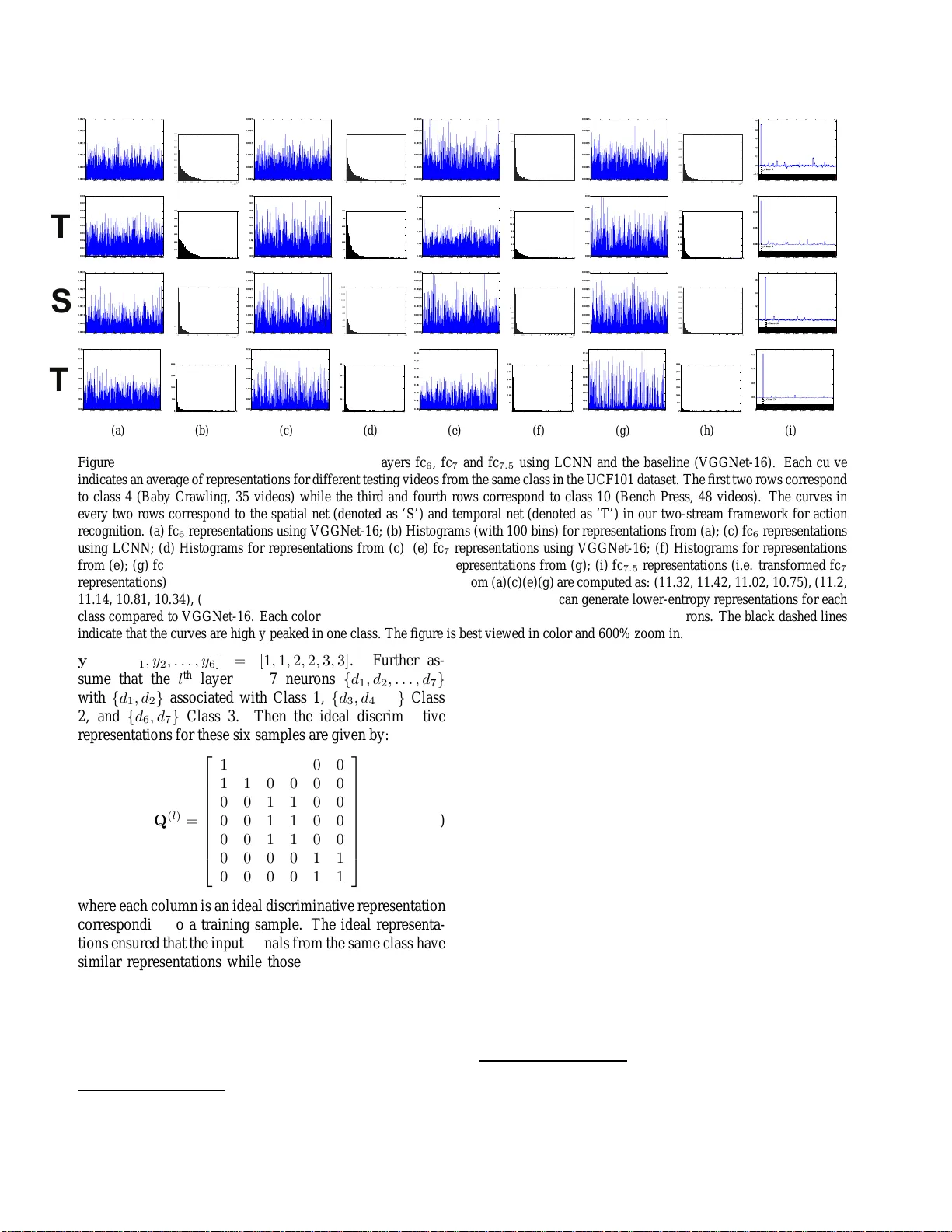
Learn ing Discriminative F eatur es via Label Consistent Neural Network Zhuolin Jiang † ∗ , Y aming W ang ‡ ∗ , Larry Da vis ‡ , W alt Andrews † , V iktor Rozgic † † Raytheon BBN T echnologies, Cambridge, MA, 02138 ‡ Univ ersity of Maryland, College P ark, MD, 20742 { zjiang,wandrews ,vrozgic } @bbn.com, { wym,lsd } @umiacs.um d.edu Abstract Deep C on volutiona l Neural Networks (CNN) enfor ce su- pervised information only at the output layer , an d hidden layers ar e trained by back pr opagatin g the pr ediction err or fr om the output layer without explicit sup ervision. W e pr o- pose a s upervised featur e learning appr oach, Label C onsis- tent Neural Network, which enfor ces dir ect supervision in late hidden layers in a n ovel wa y . W e associa te e ach n eur on in a hidden layer with a particula r class lab el and enco ur - age it to be activa ted for input signa ls fr o m the same class. Mor e specifically , we intr o duce a label con sis tency r e gular- ization called “discriminative r epresentation err or” loss for late hid den layers an d co mbine it with classification err or loss to build our overall objective fun ction. This label con- sistency constraint alleviates the common pr ob lem of gradi- ent vanishing and tends to faster conver gence; it also makes the fea tur es d erived fr om late hid den layers discriminative enoug h for classification even u sing a simple k -NN classi- fier , since in put signa ls fr om the same class will have very similar repr esentation s. Experimenta l r esults demon str a te that our app r o ach achieves state-o f-the-art performances on several pu blic benchma rks for ac tion an d object cate- gory r ecogn ition. 1. Intr oduction Con volutional neural networks (CNN) [ 20 ] have ex- hibited impressive p erformances in many compu ter vision tasks such as im age classification [ 17 ], o bject detection [ 5 ] and image retrieval [ 27 ]. When large amoun ts o f trainin g data are available, CNN can autom atically learn h ierarchi- cal featur e representatio ns, w hich are more d iscriminati ve than previous han d-crafted ones [ 17 ]. Encour aged by their impressi ve per formance in static image analy sis tasks, se veral CNN-based approac hes have been developed for action recogn ition in video s [ 12 , 15 , 25 , 28 , 35 , 44 ]. Althou gh p romising results have been re - ported, the ad v an tages of CNN appr oaches over traditional ones [ 34 ] are not as overwhelm ing for vide os as in static images. Comp ared to static image s, videos have larger v ari- ations in appea rance as well as hig h complexity introduced by tempora l evolution, which m akes learning featu res for recogn ition f rom vid eos mor e challengin g. On the other ∗ Indicat es equal contribut ions. hand, un lik e large-scale and diverse static image data [ 2 ], annotated data for action recog nition tas ks is usually in suf- ficient, since anno tating massive videos is proh ibiti vely ex- pensive. Ther efore, with only li mited annotated data, learn- ing discriminative features via deep neural network can lead to severe overfitting and slow convergence. T o tackle the se issues, previous works have introdu ced effective practical technique s such as ReLU [ 24 ] an d Drop-out [ 10 ] to im- prove the perform ance of neu ral networks, but have not con- sidered dire ctly improving the discriminative capab ility of neuron s. The featu res fr om a CNN ar e learn ed by back - propag ating pre diction error from the output layer [ 19 ], and hidden layers receive no dir ect guidan ce on class in forma- tion. W o rse, in very deep networks, the early h idden layers often suffer fro m vanishing gradients, wh ich leads to slow optimization co n vergence an d the network co n verging to a poor local minimu m. Ther efore, the quality of th e lea rned features of the hidden layers might be potentially dimin- ished [ 43 , 6 ]. T o tackle these p roblems, we pr opose a new supe rvised deep neu ral n etw ork, Lab el Consistent Neural Network , to lear n discriminative features f or recog nition. Our ap- proach provides explicit supervision, i.e . label inform ation, to late hidd en layers, by incorp orating a label con sist ency constraint called “discrimin ati ve repr esentation error” loss, which is co mbined with the classification loss to form th e overall objective functio n. Th e benefits of our approa ch are two-fold: (1) with explicit supervision to hid den layers, the problem of vanishing gra dients can be alleviated and faster conv ergence is observed; (2) mo re d iscriminati ve late h id- den layer featur es lead to incr eased discriminative po we r of classifiers at the outpu t layer ; interestingly , the learned d is- criminative feature s alon e can achiev e g ood classification perfor mance ev en with a simple k -NN classifier . In prac- tice, our ne w for mulation can be easily incorp orated into any neural network trained using backpropaga tion. Our ap- proach is ev aluated o n pu blicly available action and object recogn ition datasets. Although we only present experim en- tal results for action and object recognition , the method can be app lied to other tasks such as im age retr ie val, co mpres- sion, restorations etc ., since it generates class-specific com- pact representatio ns. 1 1.1. Main Contrib utions The main contributions of LCNN are three-fold. • By adding explicit super vision to late h idden lay ers via a “discrimin ati ve representatio n error”, LCNN learn s more discriminative features resulting in better clas- sifier tr aining at the outpu t laye r . The representa- tions generated by late hid den layers are discrimina ti ve enoug h to achie ve goo d pe rformance using a simple k - NN classifier . • The label consistency constrain t alleviates the pro blem of vanishing gradien ts and leads to faster conver gence during train ing, espe cially when limited tr aining data is av ailable. • W e achieve state-of-the-art perfo rmance on several ac- tion and o bject category recognition tasks, and the compact class-specific repr esentations g enerated by LCNN can be directly used in other application s. 2. Related W ork CNNs have achieved perfo rmance improvements over traditional h and-crafted featur es in image recognitio n [ 17 ], detection [ 5 ] and retrieval [ 27 ] etc . This is d ue to the av ail- ability of large-scale image datasets [ 2 ] an d r ecent techni- cal imp rovements s uch as ReLU [ 24 ], d rop-out [ 10 ], 1 × 1 conv olu tion [ 23 , 32 ], batch nor malization [ 11 ] and data a ug- mentation based on random flipping, RGB jittering, contr ast normalizatio n [ 17 , 23 ], which h elps speed up conv ergence while a voiding ov erfitting. AlexNet [ 17 ] initiated the dramatic performan ce im- provements of CNN in static image recognition and cur rent state-of-the- art p erformance h as been ob tained by deep er and more sop histicated n etw ork architectu res su ch as VG- GNet [ 29 ] an d GoogLeNet [ 3 2 ] . V ery recently , researche rs have applied CNNs to actio n and event recognitio n in videos. W hile in itial a pproaches use im age-trained CNN models to extract frame- le vel featur es an d aggregate them into vid eo-le vel descripto rs [ 25 , 4 4 , 38 ], more recent work trains CNNs using vide o data and f ocuses on effecti vely incorpo rating the temp oral d imension and learnin g go od spatial-tempor al features autom atically [ 12 , 15 , 28 , 3 6 , 41 , 35 ]. T wo-stream CNNs [ 28 ] are perhaps the most success- ful a rchitecture f or action reco gnition curren tly . They co n- sist of a spatial net trained with vid eo fr ames and a temporal net trained with optical flo w fields. With the two stream s capturing spatial an d temporal in formation separately , the late fusion of the two produces competitive actio n reco g- nition results. [ 36 ] and [ 41 ] have obtained fu rther p erfor- mance gain by explorin g deepe r tw o -stream network archi- tectures and refinin g technical d etails; [ 3 5 ] achieved state- of-the- art in action recog nition by integrating two-stream CNNs, improved trajectories and Fisher V ecto r encod ing. It is also worth co mparing our L CNN with limited prior work which aims to imp rov e the discrim inati veness of learned featu res. [ 1 ] perfo rms greedy layer-wise supervised pre-train ing as initialization an d fine-tunes the par ameters of all layers tog ether . Our work intro duces the su pervision to interm ediate layers as p art of the ob jecti ve fu nction dur- ing training a nd can be optimized b y bac kpropagation in an integrated way , rathe r than layer-wise greed y p retrain- ing and then fine-tu ning. [ 40 ] rep laces the o utput softm ax layer with an erro r -co rrecting coding layer to prod uce error correcting codes as network outpu t. Their network is still trained by back-p ropagating the error a t th e ou tput an d n o direct super vision is a dded to hidden layers. Deeply Su- pervised Net (DSN) [ 21 ] intr oduces an SVM c lassi fier for each hidden layer, and the fi nal ob jecti ve function is the lin- ear combin ation of th e pred iction losses at all hid den lay- ers and outp ut layer . Using all-layer sup ervision, balancing between multiple lo ss es migh t be ch allenging and the n et- work is non-tr i vial to tu ne, since o nly the classifier at the output layer will be u sed at test time an d the effects of the classifiers at hidd en layer s are difficult to ev aluate. Simi- larly , [ 31 ] also add s identification an d verification superv i- sory signals to each hidden layer to extract face rep resen- tations. In ou r work, instead of adding a p rediction loss to each hidd en layer , we intro duce a novel representation loss to g uide the form at of the learn ed features at late h idden layers only , since early layers of CNNs tend t o capture low- lev el edges, cor ners and mid- le vel parts and they should b e shared acr oss categories, while the late hidden layers ar e more class-specific [ 43 ]. 3. Featur e Learning via Supervised Deep Neu- ral Network Let ( x , y ) deno te a training s ample x an d its label y . For a CNN with n layers, let x ( i ) denote the o utput o f the i th layer and L c its objective fu nction. x (0) = x is the input data an d x ( n ) is th e outp ut o f the ne tw ork. Therefore, the network architecture can be concisely expressed as x ( i ) = F ( W ( i ) x ( i − 1) ) , i = 1 , 2 , ..., n (1) L c = L c ( x , y , W ) = C ( x ( n ) , y ) , (2) where W ( i ) represents the network parame ters of the i th layer, W ( i ) x ( i − 1) is the linear oper ation ( e.g. conv olu - tion in conv o lutional layer, or linear transfor mation in fully- connected lay er), and W = { W ( i ) } i =1 , 2 ,...,n ; F ( · ) is a non-lin ear activ atio n functio n ( e.g. ReLU) ; C ( · ) is a pre- diction err or such as softm ax lo ss. The ne tw ork is tra ined !"#$%& '!(( ) * +, - . /%0 1 ' ! (( 2 . /%, 1 3/4 5/(/0 #%#- ! 0 1 ' %6/5 )%5,617-../01'%6/5( '%#/17-../01'%6/5( 8*#4*#1'%6/5 '%9/,1:!0(-(#/0+61;!.*,/ ! " <-./!1'%9/,=1 -0? "+ @, A BC DE =1 1 F 5%0 ("! 5$/. 1 3/4 5/(/0 #%#- ! 0 1 ' %6/5 "+ @,E 1 & @,E 1 G @, E & @, E 1 "+ @,AHE 1 )*+,-./%0 1 '!(( 2./%,13/45/(/0#%#-!01'%6/5 "+ @,ABCDE =11F5%0("!5$/.13/45/(/0#%#-!01'%6/5 = 11 F 5%0 ("! 5$/. 1 3/4 5/(/0 #%#- ! 0 1 ' %6/5 G @,E & @,E I @,E Figure 1. An examp le of the L CNN structure. The label consistency module is added to the l th hidden layer , which is a fully-connected layer fc l . Its representation x l is transformed to be A ( l ) x l , which is the output of the transformed representation l aye r fc l +0 . 5 . Note that the applicability of the proposed label consistenc y module is not li mited to fully-conn ected layers. with back-pr opagation, and the gradients are computed as: ∂ L c ∂ x ( i ) = ( ∂ C ( x ( n ) ,y ) ∂ x ( n ) , i = n ∂ L c ∂ x ( i +1) ∂ F ( W ( i +1) x ( i ) ) ∂ x ( i ) , i 6 = n (3) ∂ L c ∂ W ( i ) = ∂ L c ∂ x ( i ) ∂ F ( W ( i ) x ( i − 1) ) ∂ W ( i ) , (4) where i = 1 , 2 , 3 , ..., n . 4. Label Consistent Neural Network (LCNN) 4.1. Moti vation The sparse r epresentation for classification assumes that a testing samp le can be well represented by training samples from the same class [ 37 ]. Similarly , diction ary l earning for recogn ition m aintains label informatio n f or d ictionary items during train ing in order to gen erate discriminative or class- specific sparse codes [ 14 , 39 ]. In a ne ural network, the rep - resentation of a certain layer is generated by th e neu ron acti- vations in that layer . If the class distribution for each neuron is hig hly peaked in one class, it enforces a label consistency constraint on each neuro n. This leads to a discrim inati ve representatio n over learned class-specific neuro ns. It has b een observed that ear ly hidde n layers of a CNN tend to capture low-le vel featu res shared acro ss categor ies such as edges and corners, while late hidden layers are more class-specific [ 43 ]. T o improve the discriminativeness o f features, LCNN adds explicit sup ervision to late hidden lay- ers; more s pecifically , we associate each neuron to a certain class labe l and ideally th e n euron will only ac ti vate when a sample of th e correspondin g class is presen ted. Th e label consistency con straint on neurons in LCNN will be imposed by intro ducing a “discrim inati ve representa tion erro r” loss on late h idden layers, wh ich will form part o f the o bjecti ve function during training. 4.2. Formulation The overall o bjecti ve fu nction o f LCNN is a com bina- tion of the discriminati ve rep resentation erro r at late hidden layers and the classification error at the output layer: L = L c + αL r (5) where L c in Equatio n ( 2 ) is the classification err or at the output layer , L r is the discrimin ati ve repre sentation error in Equation ( 6 ) and will be discussed in detail below , and α is a hyper parameter balancing the two terms. Suppose we want to add superv ision to the l th layer . Let ( x , y ) den ote a t raining sample and x ( l ) ∈ R N l be the corre- sponding r epresentation produ ced by the l th layer, which is defined by the activ ations of N l neuron s in that laye r . Then the discriminative r epresentation erro r is d efined to be the difference between the transform ed representatio n A ( l ) x ( l ) and the ideal discriminative representation q ( l ) : L r = L r ( x ( l ) , y , A ( l ) ) = k q ( l ) − A ( l ) x ( l ) k 2 2 , (6) where A ( l ) ∈ R N l × N l is a linear transformation m atrix, and the binary vector q ( l ) = [ q ( l ) 1 , . . . , q ( l ) j , . . . , q ( l ) N l ] T ∈ { 0 , 1 } N l denotes the id eal discrimin ati ve r epresentation which indicates the ideal activ atio ns of n eurons ( j denotes the ind e x of neuro n, i.e. the index o f feature dim ension). Each neuron is associated with a certain class lab el and, ide- ally , only activ ates to samples fro m that class. Theref ore, when a sample is f rom Class c , q ( l ) j = 1 if and only if the j th neuron is assigned to Class c , and neu rons associated to other classes sh ould not b e activated so that the cor re- sponding e ntry in q ( l ) is zero. No tice th at A ( l ) is the o nly parameter needed to be learne d, while q ( l ) is p re-defined based on label inform ation from training data. Suppose we have a batch o f six training samples { x 1 , x 2 , . . . , x 6 } and the class labels 0 500 1000 1500 2000 2500 3000 3500 4000 0.0000 0.0005 0.0010 0.0015 0.0020 0.0025 × 10 -3 0 0.2 0.4 0.6 0.8 1 1.2 1.4 1.6 1.8 0 100 200 300 400 500 600 700 0 500 1000 1500 2000 2500 3000 3500 4000 0.0000 0.0005 0.0010 0.0015 0.0020 0.0025 × 10 -3 0 0.5 1 1.5 2 0 100 200 300 400 500 600 700 0 500 1000 1500 2000 2500 3000 3500 4000 0.0000 0.0005 0.0010 0.0015 0.0020 0.0025 × 10 -3 0 0.5 1 1.5 2 2.5 0 200 400 600 800 1000 1200 0 500 1000 1500 2000 2500 3000 3500 4000 0.0000 0.0005 0.0010 0.0015 0.0020 0.0025 × 10 -3 0 0.5 1 1.5 2 2.5 3 0 200 400 600 800 1000 1200 0 500 1000 1500 2000 2500 3000 3500 4000 −0.1 0.0 0.1 0.2 0.3 0.4 0.5 Class 4 0 500 1000 1500 2000 2500 3000 3500 4000 0.00 0.01 0.02 0.03 0.04 0.05 0.06 0.07 0.08 0.00 0.01 0.02 0.03 0.04 0.05 0.06 0 100 200 300 400 500 600 0 500 1000 1500 2000 2500 3000 3500 4000 0.00 0.01 0.02 0.03 0.04 0.05 0.06 0.07 0.08 0.00 0.01 0.02 0.03 0.04 0.05 0.06 0.07 0.08 0 100 200 300 400 500 600 0 500 1000 1500 2000 2500 3000 3500 4000 0.00 0.02 0.04 0.06 0.08 0.10 0.00 0.01 0.02 0.03 0.04 0.05 0.06 0.07 0 200 400 600 800 1000 1200 1400 0 500 1000 1500 2000 2500 3000 3500 4000 0.00 0.02 0.04 0.06 0.08 0.10 0.00 0.02 0.04 0.06 0.08 0.10 0 200 400 600 800 1000 1200 1400 0 500 1000 1500 2000 2500 3000 3500 4000 0.00 0.05 0.10 0.15 Class 4 0 500 1000 1500 2000 2500 3000 3500 4000 0.0000 0.0005 0.0010 0.0015 0.0020 0.0025 0.0030 0.0035 × 10 -3 0 0.5 1 1.5 2 2.5 3 0 200 400 600 800 1000 1200 1400 0 500 1000 1500 2000 2500 3000 3500 4000 0.0000 0.0005 0.0010 0.0015 0.0020 0.0025 0.0030 0.0035 × 10 -3 0 0.5 1 1.5 2 2.5 3 3.5 0 200 400 600 800 1000 1200 1400 0 500 1000 1500 2000 2500 3000 3500 4000 0.0000 0.0005 0.0010 0.0015 0.0020 0.0025 0.0030 0.0035 × 10 -3 0 0.5 1 1.5 2 2.5 3 3.5 0 200 400 600 800 1000 1200 1400 1600 1800 0 500 1000 1500 2000 2500 3000 3500 4000 0.0000 0.0005 0.0010 0.0015 0.0020 0.0025 0.0030 0.0035 × 10 -3 0 0.5 1 1.5 2 2.5 3 3.5 0 200 400 600 800 1000 1200 1400 1600 1800 0 500 1000 1500 2000 2500 3000 3500 4000 0.0 0.2 0.4 0.6 Cla ss 1 0 0 500 1000 1500 2000 2500 3000 3500 4000 0.00 0.02 0.04 0.06 0.08 0.10 0.12 (a) 0.00 0.01 0.02 0.03 0.04 0.05 0.06 0.07 0.08 0.09 0 500 1000 1500 2000 (b) 0 500 1000 1500 2000 2500 3000 3500 4000 0.00 0.02 0.04 0.06 0.08 0.10 0.12 (c) 0.00 0.02 0.04 0.06 0.08 0.10 0.12 0 500 1000 1500 2000 (d) 0 500 1000 1500 2000 2500 3000 3500 4000 0.00 0.02 0.04 0.06 0.08 0.10 0.12 0.14 (e) 0.00 0.02 0.04 0.06 0.08 0.10 0 500 1000 1500 2000 2500 3000 (f) 0 500 1000 1500 2000 2500 3000 3500 4000 0.00 0.02 0.04 0.06 0.08 0.10 0.12 0.14 (g) 0.00 0.02 0.04 0.06 0.08 0.10 0.12 0.14 0.16 0 500 1000 1500 2000 2500 3000 (h) 0 500 1000 1500 2000 2500 3000 3500 4000 0.00 0.05 0.10 0.15 C lass 1 0 (i) Figure 2. Examples of learned representations fr om layers fc 6 , fc 7 and fc 7 . 5 using LCNN and t he baseline (VGGNet-16). Each curve indicates an a verag e of represen tations for different testi ng videos from the same class in the UCF101 d ataset. T he fi rst two rows correspond to class 4 (B aby Crawling, 35 videos) while t he third and fourth rows correspond to class 10 (Bench P ress, 48 videos). The curves in e very two rows correspond to the spatial net (denoted as ‘S’ ) and temporal net (denoted as ‘T’) in our two-stream f rame work for action recognition. (a) fc 6 representations using VGGNet-16; (b) Histograms (with 1 00 bins) for representations from (a); (c) fc 6 representations using LCNN; (d) Histograms for representations from ( c); (e) fc 7 representations using VGGNet-16; (f) Histograms f or representations from ( e); (g) fc 7 representations using LCNN ; (h) Hist og rams for representations from (g); (i) fc 7 . 5 representations (i. e. transformed fc 7 representations) using LCNN. The en tropy value s for representations from (a)(c)(e)(g) are computed as: (11.32, 11 .42, 1 1.02, 1 0.75), (11.2, 11.14, 10.81, 10.34), (11.08, 11.35, 10.67, 10.17), ( 11 .02, 10.72, 10.55, 9.37). LCNN can generate lower -entropy represen tations f or each class compared to VGGNet-16. E ach color fr om the color bars in (i) represents one class for a subset of neurons. The black dashed lines indicate that the curves are hig hly peaked in one class. The figure is best viewe d in color and 600% zoom in. y = [ y 1 , y 2 , . . . , y 6 ] = [1 , 1 , 2 , 2 , 3 , 3] . Further as- sume that the l th layer h as 7 neurons { d 1 , d 2 , . . . , d 7 } with { d 1 , d 2 } associated with Class 1, { d 3 , d 4 , d 5 } Class 2, and { d 6 , d 7 } Class 3. Then the id eal discriminative representatio ns for these six samples are gi ven by: Q ( l ) =           1 1 0 0 0 0 1 1 0 0 0 0 0 0 1 1 0 0 0 0 1 1 0 0 0 0 1 1 0 0 0 0 0 0 1 1 0 0 0 0 1 1           , (7) where each column is an ideal discrim inati ve representatio n correspo nding to a train ing samp le. Th e id eal r epresenta- tions ensured that the input signals from the same class hav e similar represen tations while those fro m different classes have dissimilar representation s. The d iscriminati ve repr esentation erro r ( 6 ) forc es the learned repr esentation to appr oximate the ideal discrimin a- ti ve rep resentation, so that the r esulting ne urons have th e label co nsistency p roperty [ 14 ], i.e. the class d istrib u tions of each neur on 1 from layer l are extreme ly peaked in one 1 Similar to computing the class distrib utions for dictionary items class. In addition, with more discriminative re presentations, the classifier , especially linear class ifiers, at the output layer can a chie ve b etter perfo rmance. Th is is because the dis- criminative pro perty of x ( l ) is very imp ortant for th e per- forman ce of a linear classifier . An example o f the LCNN arch itecture is shown in Fig- ure 1 . T he linear tra nsformation is implemen ted as a fu lly- connected layer . W e r efer it as ‘Transformed Rep resenta- tion Lay er’. W e create a new ‘Idea l Representatio n Layer’ which transforms a class labe l into the correspon ding binary vector q ( l ) ; then we feed the o utputs o f these tw o layers into the Euclidean loss layer . In o ur experim ents, we a llocate the neuron s in th e late hidden layer to each class as follows: assuming N l neuron s in that layer and m classes, we first a llocate ⌊ N l /m ⌋ neu- rons to e ach c lass and then a llocate th e remaining ( N l − m ⌊ N l /m ⌋ ) neuro ns to the top ( N l − m ⌊ N l /m ⌋ ) classes with high intra- class app earance variation. Therefo re each neuron in the late hid den layer is associated with a category label, but an inpu t signal o f a ca te gory certa inly can (and does) use all ne urons (learned features), as the representa- in [ 26 ], the class distrib utions of each neurons from the l th layer can be deri ved by measurin g their acti vation s x ( l ) ov er input signals correspond- ing to dif ferent classes. Figure 3. Class 4 (Baby Crawling) and class 10 (Bench Press) sam- ples from the UCF101 action dataset. tions in Figu re 2(i) illustrate, i.e. sharin g featu res between categories is not prohibited. 4.3. Network T ra ining LCNN is train ed via stochastic gradien t d escent. W e need to compu te the gradients of L in Equation ( 5 ) w .r . t. all the network parameter s { W , A ( l ) } . Compare d with stan- dard CNN, th e d if f erence lies in two gra dient ter ms, i.e. ∂ L ∂ x ( l ) and ∂ L ∂ A ( l ) , since x ( l ) and A ( l ) are th e only param- eters which are r elated to the newly added discrimin ati ve error L r ( x ( l ) , y , A ( l ) ) and the other pa rameters act ind e- penden tly from it. It follows fro m Equations ( 5 ) and ( 6 ) that ∂ L ∂ x ( i ) = ( ∂ L c ∂ x ( i ) , i 6 = l ∂ L c ∂ x ( l ) + 2 α ( A ( l ) x ( l ) − q ( l ) ) T A ( l ) , i = l (8) ∂ L ∂ W ( i ) = ∂ L c ∂ W ( i ) , ∀ i ∈ { 1 , 2 , ..., n } (9) ∂ L ∂ A ( l ) = 2 α ( A ( l ) x ( l ) − q ( l ) ) x ( l )T , (10) where ∂ L c ∂ x ( i ) and ∂ L c ∂ W ( i ) are co mputed by Equatio ns ( 3 ) and ( 4 ), respectiv ely . 5. Experiment s W e ev alua te our ap proach on two action recogn ition datasets: UCF101 [ 30 ] an d THUMOS15 [ 8 ], and thr ee ob- ject category datasets: Cifar - 10 [ 16 ], Image Net [ 2 ] and Cal- tech101 [ 22 ]. Our i mplementatio n o f LCNN is based on the CAFFE toolbox [ 13 ]. T o verify the ef f ecti veness of our label consistency mod - ule, we train LCNN in two ways: (1 ) W e use the discrim- inativ e rep resentation er ror loss L r only; (2 ) W e use th e combinatio n of L r and the softm ax classification erro r loss L c as in Eq uation ( 5 ). W e refer to the n etw orks trained in these ways as ‘ LCNN-1’ and ‘ LCNN-2’, respec ti vely . The baseline is to u se the softm ax classification err or loss L c only during network training. W e refer to it as ‘baseline’ in the following. Note that the baseline and LCNN are trained with the same p arameter setting and initial mode l in all ou r experiments. For action and object recognition, we introdu ce two clas- sification appro aches he re: (1) argmax : we follo w the stan- dard CNN practice of takin g th e class label cor responding to Network Architecture Sp atial T emporal Both ClarifaiNet [ 28 ] 72.7 81 87 VGGNet-19 [ 41 ] 75.7 78.3 86.7 VGGNet-16 [ 36 ] 79.8 85.7 90.9 VGGNet-16* [ 36 ] - 85.2 - baseline 77.48 83.71 - LCNN-1 80.1 8 5.59 89.87 LCNN-2 (argmax) 80.7 8 5.57 91.12 LCNN-2 ( k -NN) 81.3 8 5.77 89.84 T able 1. Classification performanc e with different two-stream CNN approaches on the UCF101 dataset (split -1). The results of [ 28 , 36 , 41 ] are c opied from their original pap ers. T he VGGNet- 16* result i s obtained by testing the model shared by [ 36 ]. The ‘baseline’ are the results of running the two-stream C NN imple- mentation provid ed by [ 36 ], where the VGGNet-16 architecture is used for each stream. LCNN and baseline are trained with the same parameter setting and initial model. The only difference be- tween L CNN-2 and the baseline is that we add e xplicit sup ervision to fc 7 layer for L CNN-2. For LCNN-1, we remov e the softmax layer from the base line netwo rk but add explicit sup ervision to fc 7 layer . Method Acc. (%) Method Acc. (%) Karpathy [ 15 ] 65.4 W ang [ 3 4 ] 85.9 Donahu e [ 3 ] 82.9 Lan [ 18 ] 89.1 Ng [ 25 ] 8 8.6 Z ha [ 44 ] 89.6 LCNN-2 (argmax) 91.12 T able 2. Recognition performance comparisons with other state- of-the-art approaches on the UCF 10 1 dataset. The results of [ 15 , 34 , 3 , 18 , 25 , 44 ] are copied from their original papers. the max imum prediction s core; (2) k -NN : W e use the t rans- formed repr esentation A ( l ) x ( l ) to repr esent an image, video frame or optical flow field and then use a simple k -NN clas- sifier . LCNN-1 always uses ‘ k -NN’ for classification wh ile LCNN-2 can u se either ‘ argmax’ or ‘ k -NN’ to do classifi- cation. 5.1. Action Recognition 5.1.1 UCF101 Data set The UCF101 dataset [ 30 ] consists of 13 , 320 vide o clips from 101 actio n classes, and every class has more than 100 clips. Some video examples fr om class 4 and c lass 10 are giv en in Figure 3 . In terms of ev alu ation, we use the stan- dard split-1 train/test setting to e valuate our approach . Split- 1 co ntains around 10 , 00 0 clip s for tr aining and the rest for testing. W e choose th e p opular two-stream CNN as in [ 28 , 36 , 41 ] as ou r ba sic ne tw ork architectur e for action rec ogni- tion. It consists of a spatial net taking video fram es as in - put and a tempor al net takin g 10 -frame stacking of op tical flow fields. Late f usion is cond ucted on th e ou tputs of th e Epoch 0 20 40 60 80 100 120 Training Error 0 1 2 3 4 5 VGGNet-16 LCNN (a) Epoch 0 20 40 60 80 100 120 Test Error 0.5 1 1.5 2 2.5 3 3.5 4 4.5 5 VGGNet-16 LCNN (b) Figure 4. Training and testing errors of spatial net trained by LCNN-2 and the baseline (VGGNet-16) on the UCF101 dataset. (a) T raining error comparison; (b) T esting error comparison. k 0 5 10 15 20 Accuracy 0.76 0.78 0.8 0.82 0.84 0.86 0.88 Spatial Net Temporal Net Figure 5. Effects of parameter selection of k -NN neighborhood size k on the classification accu racy perfo rmances on the UCF101 dataset. The spatial and temporal nets trained by L CNN-2 are not sensitiv e to the selection of k . two strea ms and generates the final predictio n score. Dur - ing testing, we sample 2 5 fram es (imag es or optical flow fields) from a video as in [ 28 ] for spatial and temporal nets. The class scores for a testing video is obtained by a veragin g the scores across samp led fr ames. In our experiments, we fuse spatial and temporal net pred iction scores using a sim- ple we ighted average rule, w here the weight is set to 2 for temporal net and 1 for spatial net. W e use the VGGNet-16 architectur e [ 29 ] as in [ 36 ] f or two streams wh ere th e explicit supervision is added in the late hidden layer fc 7 , which is the secon d fully -connected layer . Mo re specifically , we feed th e outp ut of layer fc 7 to a fully-con nected layer (denoted as fc 7 . 5 ) to prod uce the transform ed repr esentation, and compar e it to the ideal d is- criminative rep resentation q ( fc7 ) . The implem entation of this explicit sup ervision is shown in Figure 6(a) . Since UCF101 has 1 01 classes and the fc 7 layer of VGGNet h as output dimension 4096 , the output of fc 7 . 5 has the same size 4096 , and arou nd 40 n eurons ar e associated to e ach class. For both streams, we set α = 0 . 05 in ( 5 ) to balance the two loss terms. Benefits of Adding E xplicit Sup ervision to Late Hid den Layers. W e aim to dem onstrate the b enefits of ad ding ex- plicit supervisio n to late hidd en laye rs. W e first obtain the baseline result by ru nning the stand ard two-stream CNN implementatio n provided by [ 36 ], which uses softmax clas- sification lo ss o nly to train the spatial and temporal nets. Then we re mov e the softma x la yers from this two-stream CNN but add explicit supervisio n to the fc 7 hidden layers. W e call this n etwork as ‘LCNN- 1’. Next we main tain the softmax layers in the standard tw o-stream CNN b u t add ex- plicit superv ision to the fc 7 layers. W e call this n etw ork as ‘LCNN-2’. Please note that we do use the same para meter setting a nd in itial mo del in these three types o f neura l net- works. The results a re summarize d in T able 1 . It can be seen from the r esults of LCNN-1 that even without the help o f the classifier , our lab el consistency constrain t alone is very effecti ve for lear ning discrimina ti ve feature s and ac hie ves better classification per formance than the ba seline. W e can also see that adding exp licit supervision to late hidden lay- ers not only improves the classification results at the output layer (LCNN-2 (argmax)), but also g enerates discrimin a- ti ve representation s which a chie ve better results even with a simple k -NN classifier (LCNN-2 ( k -NN)) . In addition , we c ompare LCNN with o ther state-of-th e-art appro aches in T able 2 . Discriminability of Lea rned Repr esenta tions. W e visual- ize the re presentations of test videos generated by late hid- den layer s fc 7 . 5 , fc 7 and fc 6 in Figu re 2 . It can be seen that the entries of laye r fc 7 . 5 representatio ns in Figure 2(i) are very peaked at the correspondin g class, which forms a very good approx imation to the idea l d iscriminati ve representa- tion. Please note that a video of a testing class certainly can (and does) use neur ons from other classes as shown in Fig- ure 2(i) . It indicates that sharin g features between classes is not prohibited . Further n otice th at such discrimina ti ve c apa- bility is achiev ed d uring te sting, which indicates that LCNN generalizes well witho ut se vere overfitting. For fc 7 and fc 6 representatio ns in Figures 2(c) and 2(g ) , their e ntropy has decreased, which m eans that the discrim inati vene ss of pre- vious layers benefits fro m the bac kpropagation o f the dis- Network Architecture Sp atial T emporal Both VGGNet-16 [ 3 6 ] 54.5 4 2.6 - ClarifaiNet [ 28 ] 42.3 47 - GoogLeNe t [ 32 ] 53.7 39.9 - baseline 55.8 4 1.8 - LCNN-1 56. 9 45.1 59.8 LCNN-2 (argmax) 57. 3 44.9 61.7 LCNN-2 ( k -NN) 58. 6 45.9 62.6 T able 3. Mean A verage Precision performanc e on the THUMOS15 v alidation set. The results of [ 36 , 28 , 32 ] are copied from [ 36 ]. The ‘baseline’ are the results of running the two-stream C NN imple- mentation provided by [ 36 ]. LCNN and baseline are trained with the same parameter setting and initial model. Our result 62 . 6% mAP is also better than 54 . 7% using method in [ 18 ], w hich is re- ported in [ 8 ]. criminative rep resentation error intro duced by LCNN. In Figure 5 , we plot the perform ance curves for a rang e of k (r ecall k is th e num ber of nearest neighb ors f or a k -NN classifier) using L CNN-2. W e observe that ou r approach is insensitiv e to the selection of k , lik ely due to the increase of inter-class d istances in g enerated class-specific rep resenta- tions. Smaller T raining and T esting Err ors. W e inves tigate the con vergence and testing error of LCNN durin g network training. W e plo t the testing err or and training erro r w .r .t. number of epochs f rom spatial net in Figure 4 . It can be seen that LCNN has smaller training error than the baseline (VGGNet-16), which can co n verge m ore quick ly an d alle- viate gr adient vanishing d ue to the exp licit sup ervision to late hidden lay ers. In addition , LCNN has smaller testing error compare d with the baseline , which means that LCNN has better generalization capability . 5.1.2 THUMOS15 Dataset Next we ev aluate ou r appro ach o n the more challeng ing THUMOS15 challenge action dataset. It includes all 13,320 video clips from UCF101 dataset for train ing, and 2 , 104 temporar ily untrimmed videos from the 101 clas ses for v al- idation. W e employ the standard Mean A verage Prec ision (mAP) for THUMOS15 reco gnition task to e valuate LCNN. W e use two-stream CNN based on VGGNet-16 dis- cussed in Section 5.1.1 , where explicit superv ision is added in the fc 7 layers. W e train it using all UCF101 d ata. W e used the ev aluation tool provided by the dataset provider to ev aluate mAP pe rformance, wh ich requ ires the probabilities for each category f or a testing video. For our two classifi- cation schemes, i.e. argma x an d k -NN, we use different approa ches to generate the pro bability prediction for a test- ing video. For argmax, we can direc tly use the ou tput layer . For the k -NN scheme, given the rep resentation from fc 7 . 5 layer, we com pute a sample’ s distances to classes only pre- !" #$ % &' ( )* )+#( ,- % .' / 0 $ # !"#$ !+#%1*//#(% !-#2) 3!+! 4, 5 /2'6 5 !"#$%&'()*)+#(,- %.'/0$# (a) !" #$ % &' ( )* )+#( ,- % .' / 0 $ # !"#$ !+#%1*//#(% !-#2) 3!+! ,,,4 5 5 ,,,4 6 !"#$%&'()*)+#(,- %.'/0$# 7$!++#(% !-#2 (b) !"#$%&'()*)+#(,- %.'/0$#%1 !"#$ 2!+! $'))13 4, $'))13 /5'6 4, !"#$%&'()*)+#(,- %.'/0$#%7 $'))73 4, $ ' ))7 3 $'))73 /5'6 4, 6''$83 9:9;1 6''$83 /5'6 9:9;1 !"#$%&'()*)+#(,- %.'/0$#%< *(,#6+*'(=!3 '0+60+ *(,#6+*'(=/3 '0+60+ (c) Figure 6. Examples of direct (explicit) supervision in the late hid- den layers including (a) fc 7 layer in the CNN architectures in- cluding VGGNet [ 29 ] and AlexNet [ 17 ]; ( b) CCCP5 layer in the Network-in-Netw ork [ 23 ];(c) loss 1 / fc, loss 2 / fc and Pool 5 / 7 × 7 S 1 in the GoogLeNet [ 32 ]. The symbol of three dots denotes other layers in the network. sented in its k nearest n eighbors, and convert them to simi- larity weights u sing a Gaussian kernel and set o ther classes to have very low similarity; finally we ca lculate the pro ba- bility by doing L1 norma lization on the similarity vector . W e obtained the b aseline by running the two-stream CNN implementatio n provid ed by [ 36 ]. W e co mpare our LCNN results with the baseline and o ther state-of-the-ar t approa ches [ 36 , 28 , 32 ] on the THUMOS15 dataset. The re- sults are summar ized in T able 3 . LCNN-1 is better than the baseline and LCNN-2 can further improve the mAP perfor- mances. Our results i n the spatial stream outperform the re- sults in [ 36 ], [ 28 ] and [ 32 ], while our results in the temporal stream ar e comp arable to [ 28 ]. Based on this experim ent, we can see that LCNN is high ly effectiv e and g eneralizes well to more complex testing data. 5.2. Object Recognition 5.2.1 CIF AR-10 Data set The CIF AR-10 dataset co ntains 6 0 , 0 00 colo r imag es f rom 10 classes, which are split into 50 , 00 0 tr aining images and 10,00 0 testing im ages. W e co mpare LCNN-2 with several recently pro posed techniqu es, especially the Deeply Super- Method (W itho ut Data Aug ment.) T est Error (%) Stochastic Pooling [ 42 ] 15.13 Maxout Networks [ 7 ] 11.68 DSN [ 21 ] 9.78 baseline 10.41 LCNN-2 (argmax) 9.75 Method (W ith Data Au gment.) T e st Error (%) Maxout Networks [ 7 ] 9.38 DropConn ect [ 33 ] 9.32 DSN [ 21 ] 8.22 baseline 8.81 LCNN-2 (argmax) 8.14 T able 4. T est error rates from different approache s on the CI F AR- 10 dataset. The results o f [ 42 , 7 , 33 , 21 ] are co pied from [ 23 ] . The ‘baseline’ is the result of Network in Network (NIN) [ 23 ]. Fol- lo wing [ 21 ], LCNN-2 is also trained on top of the NIN implemen - tation provide d by [ 23 ]. The only difference between the baseline and LCNN-2 is t hat we add the explicit supervision to t he cccp 5 layer for LCNN-2. vised Net (DSN) [ 21 ], which adds explicit su pervision to all hid den la yers. For our under lying architectur e, we also choose Network in Network (NIN ) [ 23 ] as in [ 21 ]. W e fo l- low the same data aug mentation technique s in [ 23 ] b y zero padding o n each side, then do corn er cropping and ran dom flipping during training. For LCNN-2, we add the explicit supervision to the 5 th cascaded cro ss chan nel p arametric p ooling layer (cccp 5 ) [ 2 3 ], which is a late 1 × 1 conv olutional layer . W e first flatten the outp ut of this c on volutional layer into a one dimensiona l vector , and then fe ed it into a fu lly-connected layer (d enoted as fc 5 . 5 ) to ob tain the transfor med represen- tation. T his imp lementation is shown in Figure 6(b) . W e set the hyper-param eter α = 0 . 03 75 d uring train ing. For classification, we adopt the argmax class ification scheme. The b aseline result is fro m NIN [ 23 ]. LCNN-2 is con- structed on top of the NIN implemen tation provid ed by [ 23 ] with the same parameter s etting and initial mod el. W e com- pare our LCNN-2 r esult with the baseline and other state- of-the- art app roaches includin g DSN [ 21 ]. The r esults ar e summarized in T able 4 . Regardless of the da ta a ugmenta- tion, LCNN-2 co nsistently o utperforms all p re v ious me th- ods, inclu ding th e b aseline NIN [ 23 ] and DSN [ 21 ]. The results are imp ressi ve, since DSN adds an SVM lo ss to ev- ery hid den layer du ring trainin g, wh ile LCNN-2 only adds a discriminative representatio n error loss to on e l ate hidden layer . It suggests that adding direct sup ervision to the m ore category-specific late hidden layers m ight be more e f fec - ti ve than to the ea rly hidden layers which tend to be shared across categories. Network Architecture T op-1 (%) T op-5 (%) GoogLeNe t [ 32 ] - 89.93 AlexNet [ 17 ] 58.9 - Clarifai [ 43 ] 62.4 - baseline 62.64 85.54 LCNN-2 (argmax) 68.68 89.03 T able 5. Recognition Performances using dif ferent approaches on the ImageNet 2012 V alidation set. The result of [ 32 ] is copied from original paper while the results o f [ 17 , 43 ] are cop ied from [ 40 ]. T he ‘baseline’ is the result of running the GoogLeNet implementation in CAFF E toolbox. The only difference between the baseline and LCNN- 2 is that we add explicit supervision to three layers (loss 1 / fc, loss 2 / fc and Pool 5 / 7 × 7 S 1 ) for LCNN-2. 5.2.2 ImageNet Dataset In this sectio n, we demonstrate that LCNN can b e com bined with state-of-the-ar t CNN architecture GoogLeN et [ 32 ], which is a most recent v ery d eep CNN with 22 layers and ach ie ved the best perf ormance on ILSVRC 2014. T he ILSVRC classification ch allenge contains abou t 1.2 m il- lion training images and 50 , 00 0 images for validation from 1,000 categories. T o tackle such a very deep network architecture, we con - struct LCNN on top o f the Goo gLeNet implementatio n in CAFFE toolbox by adding explicit sup ervision to multip le late hidden layers instead of a sing le one. Specifically , as shown in Figure 6(c) , the d iscriminati ve repr esentation er- ror losses are added to three layer s: loss 1 / fc, loss 2 / fc and Pool 5 / 7 × 7 S 1 with the same we ights used for the t hree soft- max loss layers in [ 32 ]. W e ev aluate our appr oach in terms of top-1 and top-5 accuracy rate. we adopt the ar gmax clas- sification scheme. The b aseline is the result of ru nning Go ogLeNet im- plementation in CAFFE toolbox . Our LCNN-2 and GoogLeNe t are trained on the ImageNet d ataset f rom scratch with the same parameter setting. The results are listed in T able 5 . LCNN-2 outperf orm the baseline in both evaluation m etrics with the same parameter setting. Please n ote that we did not g et the same result reported in Goo gLeNet [ 32 ] by simply run ning th e implem entation in CAFFE. Our goal here is to show that as the network becomes deeper, learning goo d discriminative features fo r hidden layers m ight b ecome mo re difficult so lely dep ending on the p rediction err or loss. Th erefore, add ing explicit su- pervision to late hid den layers under this scenario bec omes particularly useful. 5.2.3 Caltech10 1 Dataset Caltech101 contains 9 , 146 images from 101 o bject cate- gories and a b ackground categor y . In this expe riment, we test the perfo rmance of LCNN with a limited amoun t of Method Accuracy(%) LC-KSVD [ 14 ] 73.6 Zeiler [ 43 ] 86.5 Dosovitskiy [ 4 ] 85.5 Zhou [ 45 ] 87.2 He [ 9 ] 91.44 baseline 87.1 LCNN-1 ( k -NN) 88.51 LCNN-2 (argmax) 90.11 LCNN-2 ( k -NN) 89.45 baseline* 92.5 LCNN-2* (argmax) 93.7 LCNN-2* ( k -NN) 93.6 T able 6. Comparison s of LCNN with other app roaches on the Cal- tech101 dataset. The results of [ 14 , 43 , 4 , 45 , 9 ] are copied from their original pape rs. The ‘baseline’ and ‘baseline*’ are the results by fi ne-tun ing Alex Net model [ 17 ] and V GG Net-16 model [ 2 9 ] on Caltech101 dataset, respectively . LCNN-1, LCNN-2 and ‘base- line’ are trai ne d with the same parameter setting. LCNN-2 and ‘baseline*’ are trained with the same parameter setting as well. training d ata, and compare it with se veral state-of -the-art approa ches, including label consistent K-SVD [ 14 ]. For fair compar ison with previous work, we fo llo w the standard classification settings. During training time, 30 images a re ran domly chosen from each category to form the training set, an d at most 50 imag es p er category are tested. W e u se th e ImageNet train ed m odel from AlexNet in [ 17 ] an d VGGNet-16 in [ 29 ], and fine-tu ne them on the Caltech101 dataset. W e built our LCNN on to p of AlexNet and VGGNet-16 respectively in this experim ent. T he ex- plicit sup ervision is a dded to the second fu lly-connected layer (fc 7 ). W e set the hyp erparameter α = 0 . 0375 . The baseline is the result of fine-tun ing AlexNet on Cal- tech101 . Then we finetune o ur LCNN with the same param- eter setting an d initial model. Similarly , we obtain ed the baseline* result a nd LCNN results based o n VGGNet-16. The results ar e summarized in T ab le 6 . With only a limited amount of data av a ilable, our app roach makes better use of the training data and achieves higher accu racy . LCNN ou t- perfor ms b oth the baselin e results and other de ep lear ning approa ches, representing state-of-the-ar t on this task. 6. Conclusion W e intro duced th e Label Consistent Ne ural Network, a supervised featu re learning algo rithm, by ad ding explicit supervision to late hidden layers. By introd ucing a discrim- inativ e representation error and comb ining it with the tradi- tional pred iction er ror in neura l networks, we achieve bet- ter classification pe rformance at the outp ut layer , and more discriminative represen tations at the hidde n layers. Experi- mental results show that ou r approach operates at the state- of-the- art on several pub licly a vailable action and o bject recogn ition dataset. It leads to faster convergence speed and work s well when only limited vid eo or im age data is presented. Our ap proach can b e seamlessly comb ined with various network architectures. Futur e w o rk includes apply- ing the discrim inati ve learned category -specific rep resenta- tions to o ther comp uter vision tasks b esides action and ob- ject recognition . Acknowledgeme nt This work is supported by the Intelligence Advanced Re- search Projects Activity (IARP A) via Dep artment of Interior National Business Center contract n umber D11PC2007 1. The U.S. Governmen t is auth orized to repr oduce and dis- tribute reprin ts f or Government purpo ses notwithstanding any copyright anno tation thereon . Disclaimer : The views and co nclusions contained herein ar e those of the authors and should not be interpr eted as ne cessarily rep resenting the o f ficial policies or end orsements, eithe r expressed or im- plied, of IARP A, Do I/NBC, or the U.S. Go vernment. Refer ences [1] Y . Bengio, P . Lamblin, D. Popovici, and H. Larochelle. Greedy layer -wise trainin g o f d eep netw orks. In NIPS , 2006. 2 [2] J. Deng, W . Dong, R. Socher , L. Li, K. Li , and F . Li. Ima- genet: A large-scale hierarchical i mag e database. In CVPR , 2009. 1 , 2 , 5 [3] J. Donahue, L. A. Hendricks, S. Guadarrama, M. Rohrbach, S. V enugopalan , K. Saenko, a nd T . Darrell. Long-term recur - rent con volutional network s for visual recognition and de- scription. In C VPR , 2 015. 5 [4] A. Do sovitskiy , J. T . Springenber g, M. Riedmiller , and T . Br o. Discriminativ e unsupe rvised feature learning with con volutional neural network s. In NIPS , 2014. 9 [5] R. B. Girshick, J. Donahue, T . Darrell, and J. Malik. Rich feature hierarchies for accurate object detection and semantic segmen tation. In CVPR , 2014. 1 , 2 [6] X. Gl orot and Y . Bengio. Understan ding the difficulty of training deep feedforward neural networks. In AIST ATS , 2010. 1 [7] I. J. Goodfello w , D. W arde-Farley , M. Mirza, A. C. Courville, an d Y . Beng io. Maxout netw orks. In ICML , 2013. 8 [8] A. Gorban, H. Idrees, Y .-G. Jiang, A. Roshan Z amir , I. Laptev , M. S hah , and R. Sukthank ar . THUMOS chal- lenge: Action recognition wit h a large number of classes. http://www.th umos.info/ , 2015. 5 , 7 [9] K. He, X. Zhang, S. Ren, and J. Sun . Spatial pyramid pooling in deep conv olutional networks for visual recognition. In ECCV , 2014. 9 [10] G. E. Hinton , N. Sri vastav a, A. Krizhe vsky , I. Sutske ver , and R. Salakhutdinov . Improving neural networks by prev enting co-adaptation of feature detectors. arXiv: 1207.0580 , 2012. 1 , 2 [11] S. Ioffe and C. S ze gedy . Batch normalization: Accelerating deep netw ork training by reducing internal co variate sh ift. In ICML , 2015. 2 [12] S. Ji , W . Xu, M. Y ang, and K. Y u. 3d con volutional neural networks for huma n action recognition. In ICML , 2 010. 1 , 2 [13] Y . Jia, E. Shelhamer , J. Donahue, S. Karayev , J. Long, R. B. Girshick, S . Guadarrama, and T . Darrell. Caf f e: Con volu- tional architecture for fast feature embedding. In ACM MM , pages 675– 678, 2014. 5 [14] Z. Jiang, Z. Lin, and L. S. Davis. Learning a discriminative dictionary for sparse coding via label consistent K-SVD. In CVPR , 2011. 3 , 4 , 9 [15] A. Karpathy , G. T oderici, S. Shetty , T . Leung , R. Sukthankar , and F . Li. Large-scale video classification with c on volutional neural network s. In CVPR , 20 14. 1 , 2 , 5 [16] A. Krizhevsk y and G. Hinton. Learning multiple layers of features from tiny images. T echnical Report, 2009. 5 [17] A. Krizhevsk y , I. Sutske ver , and G. E. Hinton. Imagen et classification wi th deep con volutional neural networks. In NIPS , 2012. 1 , 2 , 7 , 8 , 9 [18] Z. Lan, M. Lin, X. L. A. G. Hauptmann, and B. Raj. Be- yond gaussian pyram id: Multi-skip feature stacking for ac- tion recognition. In CVPR , 20 15. 5 , 7 [19] Y . LeCun, B. E. Boser, J. S. Denker , D. Henderson, R. E. Ho ward, W . E. Hubbard, and L. D. Jackel. Backpropagation applied to hand written zip co de recog nition. Neural Compu - tation , 1(4):541 –551, 1989. 1 [20] Y . L ecu n, L. Bottou, Y . Bengio, and P . Haffner . Gradient- based learning applied t o document recognition. P r oceed- ings of the IEEE , 86(11):227 8–2324 , Nov 1998. 1 [21] C. Lee, S. Xie, P . W . Gallagher , Z. Zhang, and Z. Tu. Deeply- supervised nets. In A IST A TS , 2015. 2 , 8 [22] F . Li, R. Fergus, and P . Perona. One-shot l earnin g of ob- ject categ ories. IEEE T rans. P attern A na l. Mach . Intell. , 28(4):594–6 11, 2006. 5 [23] M. Lin, Q. Che n, and S. Y an. Network in netw ork. In IC LR , 2014. 2 , 7 , 8 [24] V . Nair and G. E. H inton . Rectifi ed linear units improve re- stricted boltzmann machines. In ICML , 2010. 1 , 2 [25] J. Y . Ng, M. J. Hausknecht, S. V ijayanarasimhan, O. Vin yals, R. Monga, and G. T oderici. Bey ond short snippets: Deep networks for video classification. In CVPR , 201 5. 1 , 2 , 5 [26] Q. Qiu, Z. Jiang, and R . Chellappa. Sparse dictionary-based representation and recognition of action attributes. In ICCV , 2011. 4 [27] A. S. Razavian, J. Sulliv an, A. Maki, and S. Carl sson . Rich feature hierarchies for accurate ob ject detection and sem antic segmen tation. In ICLR , 2015. 1 , 2 [28] K. S imon yan and A. Zisserman. T wo-stream conv olutional networks for action recognition in vide os. In NIPS , 2014. 1 , 2 , 5 , 6 , 7 [29] K. Simonyan and A. Zisserman. V ery deep con volu- tional networks for large-scale image recognition. CoRR , abs/1409.15 56, 2014. 2 , 6 , 7 , 9 [30] K. Soomro, A. Roshan Z amir , and M. S hah . UCF101: A dataset of 101 human action s classes from video s in the wild. In CRCV -T R-12-01 , 201 2. 5 [31] Y . Sun, X. W ang, and X. T ang. Deeply learned face repre- sentations are sparse, selecti ve, and r ob ust. In C VPR , 2015. 2 [32] C. Szege dy , W . Liu, Y . Jia, P . Sermanet, S. Reed, D. Anguelov , D. Erhan, V . V anhoucke, and A. Rabinovich. Going deeper with con volutions. In CVPR , 2015. 2 , 7 , 8 [33] L. W an, M. D. Z eiler , S. Zhang, Y . LeCun, and R. Fergus. Regularization of neural network s using dropco nnect. I n ICML , 2013. 8 [34] H. W ang and C. Schmid. Action recognition wit h improv ed trajectories. In ICCV , 2 013. 1 , 5 [35] L. W ang, Y . Qiao, and X. T ang. Action recognition wit h trajectory-pooled deep-con volutional descriptors. In CVPR , 2015. 1 , 2 [36] L. W ang, Y . Xiong, Z. W ang, and Y . Qiao. T o wards Good Practices f or V ery Deep T wo-Stream C on vNets. arXiv: 1507.021 59 , 2015. 2 , 5 , 6 , 7 [37] J. Wright, A. Y . Y ang, A. Ganesh, S . S . S astry , and Y . Ma. Robust face recognition via sparse representation. TP AMI , 31(2):210–2 27, 2009. 3 [38] Z. Xu, Y . Y ang, and A. G. Hauptmann. A discriminati ve CNN video representation for ev ent detection. CVPR , 2015. 2 [39] M. Y ang, L. Zhang, X. Feng, and D. Zhang. Fisher dis- crimination dictionary learning for sparse representation. In ICCV , 2011. 3 [40] S. Y ang, P . Luo, C. C. Loy , K. W . Shum, and X. T ang. Deep representation lea rning with tar get co ding. In AAAI , 2015. 2 , 8 [41] H. Y e, Z. W u, R. Zhao , X. W ang, Y . Jiang , an d X. Xue. Eval- uating two-stream CNN for video classifi cation. In ICMR , 2015. 2 , 5 [42] M. D. Zeiler and R. Fergus. S tochastic pooling for regu- larization of deep con volutional neural networks. In IC LR , 2013. 8 [43] M. D. Z eiler and R. Fergus. V i sualizing and understanding con volutional networks. In EC CV , 201 4. 1 , 2 , 3 , 8 , 9 [44] S. Z ha, F . Luisier , W . Andrews, N. Sriv astava, and R. Salakhutdinov . Exploiting image-trained CNN architec- tures fo r un constrained video classification. In BMVC , 2015. 1 , 2 , 5 [45] B. Zhou, A . Lapedriza, J. Xiao, A. T orralba, and A . Oliv a. Learning deep features for scene recognition using places database. In NIPS , 2014. 9