When Does a Boltzmannian Equilibrium Exist?

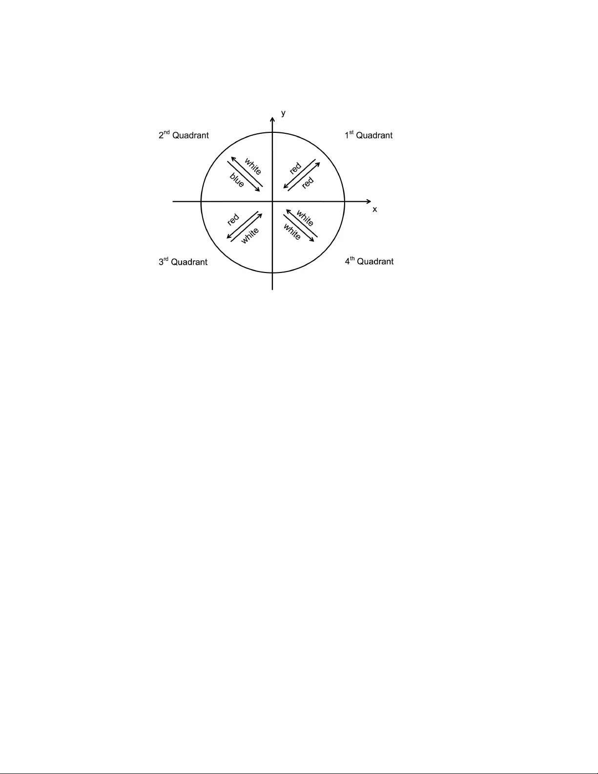
When Do es a Boltzmannian Equilibrium Exist? Charlotte W erndl ∗ and Roman F rigg † T o b e published in: Daniel Bedingham, Ow en Maroney and Christopher Timpson (eds.): Quantum F oundations of Statistic al Me chanics , Oxford: Oxford Universit y Press. Con ten ts 1 In tro duction 2 2 Boltzmannian Equilibrium 2 3 The Existence of an Equilibrium Macro-State 6 3.1 The Holist T rinity . . . . . . . . . . . . . . . . . . . . . . . . . . . . . 7 3.2 The Existence Theorem . . . . . . . . . . . . . . . . . . . . . . . . . 9 4 T o y Example: The Ideal P endulum 10 5 A F resh Lo ok at the Ergo dic Programme 18 6 Gases 19 6.1 The Dilute Gas . . . . . . . . . . . . . . . . . . . . . . . . . . . . . . 19 6.2 The Ideal Gas . . . . . . . . . . . . . . . . . . . . . . . . . . . . . . . 22 6.3 The Kac Gas . . . . . . . . . . . . . . . . . . . . . . . . . . . . . . . 24 6.4 Gas of Noninteracting Particles in a Stadium-Bo x . . . . . . . . . . . 25 6.5 Gas of Noninteracting Particles in a Mushro om-Bo x . . . . . . . . . . 26 6.6 Gas of Noninteracting Particles in a Multi-Mushro om-Bo x . . . . . . 27 7 Conclusion 29 ∗ Departmen t of Philosophy , Universit y of Salzburg and Departmen t of Philosophy , Logic and Scienic Metho d, London Sc ho ol of Economics and Political Science, c harlotte.werndl@sbg.ac.at. † Departmen t of Philosophy , Logic and Scientic Metho d, and Centre for Philosoph y of Natural and So cial Science, London Sc ho ol of Economics and Political Science. r.p.frigg@lse.ac.uk. 1 1 In tro duction The receiv ed wisdom in statistical mec hanics (SM) is that isolated systems, when left to themselves, approach equilibrium. Bu t under what circumstances do es an equilib- rium state exist and an approach to equilibrium take place? In this pap er we address these questions from the v an tage p oint of the long-run fraction of time definition of Boltzmannian equilibrium that we dev elop ed in tw o recent pap ers (W erndl and F rigg 2015a, 2015b). After a short summary of Boltzmannian statistical mec hanics (BSM) and our definition of equilibrium (Section 2), we state an existence theorem which pro vides general criteria for the existence of an equilibrium state (Section 3). W e first illustrate how the theorem works with a to y example (Section 4), whic h allows us to illustrate the v arious elemen ts of the theorem in a simple setting. After com- men ting on the ergo dic programme (Section 5) w e discuss equilibria in a num b er of differen t gas systems: the ideal gas, the dilute gas, the Kac gas, the stadium gas, the m ushro om gas and the multi-m ushro om gas (Section 6). In the conclusion w e briefly summarise the main p oints and highligh t op en questions (Section 7). 2 Boltzmannian Equilibrium Our focus are systems whic h, at the micro lev el, are measure-preserving deterministic dynamical systems ( X , Σ X , µ X , T t ). 1 The set X represen ts all p ossible micro-states; Σ X is a σ -algebra of subsets of X ; the evolution function T t : X → X , t ∈ R (con tin uous time) or Z (discrete time) is a measurable function in ( t, x ) such that T t 1 + t 2 ( x ) = T t 2 ( T t 1 ( x )) for all x ∈ X and all t 1 , t 2 ∈ R or Z ; µ X is a measure on Σ X , whic h is inv arian t under the dynamics. That is, µ X ( T t ( A )) = µ X ( A ) for all A ∈ Σ X and all t . 2 The function s x : R → X or s x : Z → X , s x ( t ) = T t ( x ) is called the solution through the p oint x ∈ X . A set of macro-v ariables { v 1 , ..., v l } ( l ∈ N ) characterises the system at the macro- lev el. The fundamen tal p osit of BSM is that macro-states sup erv ene on micro-states, implying that a system’s micro-state uniquely determines its macro-state. Th us the macro-v ariables are measurable functions v i : X → V i , asso ciating a v alue with a p oin t x ∈ X . Capital letters V i will b e used to denote the v alues of v i . A particular set of v alues { V 1 , ..., V l } defines a macr o-state M V 1 ,...,V l . If the specific v alues V i do not matter, w e only write ‘ M ’ rather than ‘ M V 1 ,...,V l ’. F or now all we need is the general definition of macro-v ariables. W e will discuss them in more detail in Sections 3 and 4, where we will see that the c hoice of macro-v ariables is a subtle and imp ortan t matter 1 This section is based on W erndl and F rigg (2015a, 2015b). F or a discussion of sto c hastic systems see W erndl and F rigg (2016). 2 A t this p oint the measure need not b e normalised. 2 and that the nature as well as the existence of an equilibrium state crucially dep ends on it. The determination relation b et w een micro-states and macro-states will nearly alw a ys b e many-to-one. Therefore, every macro-state M is asso ciated with a macro- region consisting of all micro-states for which the system is in M . A neglected but imp ortan t issue is on what space macro-regions are defined. The ob vious option would b e X , but in many cases this is not what happ ens. In fact, often macro-regions are defined on a subspace Z ⊂ X . In tuitiv ely sp eaking, Z is a subset whose states evolv e in to the same equilibrium macro-state. T o give an example: for a dilute gas with N particles X is the 6 N -dimensional space of all p osition and momenta, but Z is the 6 N − 1 dimensional energy h yp ersurface. X will b e called the ful l state sp ac e and Z the effe ctive state sp ac e of the system. The macro-region Z M corresp onding to macro-state M relative to Z is then defined as the set of all x ∈ Z for whic h M sup erv enes on x . A set of macro-states is complete relativ e to Z iff (if and only if ) it con tains all states of Z . The members of a complete set of macro-regions Z M do not o v erlap and jointly cov er Z , i.e. they form a partition of Z . Z has to be determined on a case-by-case basis, b ecause the particulars of the system under consideration determine the correct c hoice of Z . W e return to this point in Section 3. How ever, there is one general constraint on such a choice that needs to b e mentioned now. Since a system can never leav e the partition of macro-regions, it is clear that Z must b e mapped on to itself under T t . If such a Z is found, the sigma algebra on X can b e restricted to Z and one can consider a measure on Z whic h is inv ariant under the dynamics and normalized (i.e. µ Z ( Z ) = 1). In this wa y the measure-preserving dynamical system ( Z , Σ Z , µ Z , T t ) with a normalized measure µ Z is obtained. 3 W e call ( Z, Σ Z , µ Z , T t ) the effe ctive system (as opp osed to the ful l system ( X , Σ X , µ Z , T t )). M eq is the equilibrium macrostate and the corresp onding macro-region is Z M eq . An imp ortant asp ect of the standard presentation of BSM is that Z M eq is the largest macro-region. The notion of the ‘largest macro-region’ can b e in terpreted in t w o w a ys. First, ‘largest’ can mean that the equilibrium macro-region takes up a large part of Z . More sp ecifically , Z M eq is said to be β -dominant iff µ Z ( Z M eq ) ≥ β for a particular β ∈ ( 1 2 , 1]. If Z M eq is β -dominan t, it is clear that it is also β 0 -dominan t for all β 0 in (1 / 2 , β ). Second, ‘largest’ can mean ‘larger than any other macro-region’. W e sa y that Z M eq is δ -pr evalent iff min M 6 = M eq [ µ Z ( Z M eq ) − µ Z ( Z M )] ≥ δ for a particular δ > 0, δ ∈ R . It follows that if a Z M eq is δ -prev alen t, then it is also δ 0 -prev alen t for all 3 The dynamics is given by the evolution equations restricted to Z . W e follow the literature by denoting it again b y T t . 3 δ 0 in (0 , δ ). W e do not adjudicate b etw een these different definitions; either meaning of ‘large’ can be used to define equilibrium. How ever, w e w ould lik e to p oint out that they are not equiv alent: if an equilibrium macro-region is β -dominan t, there is a range of v alues for δ so that the macro-region is also δ -prev alen t for these v alues. Ho w ev er the conv erse fails. No w the question is: wh y is the equilibrium state β -dominant or δ -prev alent? A justification ought to b e as close as p ossible to the thermo dynamics (TD) notion of equilibrium. In TD a system is in equilibrium just in case change has come to a halt and all thermo dynamic v ariables assume constan t v alues ( cf. Reiss 1996, 3). This w ould suggest a definition of equilibrium according to whic h every initial condition lies on tra jectory for whic h { v 1 , ..., v k } even tually assume constant v alues. Y et this is unattainable for t w o reasons. First, b ecause of Poincar ´ e recurrence, the v alues of the v i will never reac h a constant v alue and k eep fluctuating. Second, in dynamical systems we cannot exp ect al l initial conditions to lie on tra jectories that approac h equilibrium (see, e.g., Callender 2001). T o do justice to these facts ab out dynamical systems we revise the TD definition sligh tly and define equilibrium as the macro-state in whic h tra jectories starting in most initial conditions sp end most of their time. This is not a feeble compromise. Exp erimen tal results sho w that ph ysical systems exhibit fluctuations a wa y from equi- librium (W ang et al. 2002). Hence strict TD equilibrium is actually unph ysical and a definition of equilibrium that mak es ro om for fluctuations is empirically more ade- quate. T o make this idea precise w e introduce the long-run fraction of time a system sp ends in a region A ∈ Σ Z when the system starts in micro-state x at time t = 0: LF A ( x ) = lim t →∞ 1 t Z t 0 1 A ( T τ ( x )) dτ for contin uous time, i.e. t ∈ R , (1) LF A ( x ) = lim t →∞ 1 t t − 1 X τ =0 1 A ( T τ ( x )) for discrete time, i.e. t ∈ Z , where 1 A ( x ) is the c haracteristic function of A , i.e. 1 A ( x ) = 1 for x ∈ A and 0 otherwise. Note that a measure-preserving dynamical system ( Z , Σ Z , µ Z , T t ) with the normalized measure µ Z is er go dic iff for any A ∈ Σ Z : LF A ( x ) = µ Z ( A ) , (2) for all x ∈ Z except for a set W with µ Z ( W ) = 0. 4 The lo cution ‘most of their time’ is b eset with the same am biguit y as the ‘largest macro-state’. On the first reading ‘most of the time’ means more than half of the total time. This leads to the following formal definition of equilibrium: BSM α - ε -Equilibrium. Consider an isolated system S whose macro-states are sp ecified in terms of the macro-v ariables { v 1 , ..., v k } and whic h, at the micro lev el, is a measure-preserving deterministic dynamical system ( Z, Σ Z , µ Z , T t ). Let α b e a real num b er in (0 . 5 , 1], and let 1  ε ≥ 0 b e a v ery small real num b er. If there is a macrostate M V ∗ 1 ,...,V ∗ k satisfying the follo wing condition, then it is the α - ε -equilibrium state of S : There exists a set Y ⊆ Z such that µ Z ( Y ) ≥ 1 − ε , and all initial states x ∈ Y satisfy LF Z M V ∗ 1 ,...,V ∗ l ( x ) ≥ α . (3) W e then write M α - ε - eq := M V ∗ 1 ,...,V ∗ k . An obvious question concerns the v alue of α . Often the assumption seems to b e that α is close to one. This is reasonable but not the only p ossible c hoice. F or our purp oses nothing hangs on a the v alue of α and so w e leav e it open what the b est c hoice would b e. On the second reading ‘most of the time’ means that the system sp ends more time in the equilibrium macro-state than in an y other macro-state. This idea can b e rendered precise as follows: BSM γ - ε -Equilibrium. Consider an isolated system S whose macro-states are sp ecified in terms of the macro-v ariables { v 1 , ..., v k } and whic h, at the micro lev el, is a measure-preserving deterministic dynamical system ( Z, Σ Z , µ Z , T t ). Let γ b e a real num b er in (0 , 1] and let 1  ε ≥ 0 b e a v ery small real n umber. If there is a macro-state M V ∗ 1 ,...,V ∗ l satisfying the follo wing condition, then it is the γ - ε equilibrium state of S : There exists a set Y ⊆ Z such that µ Z ( Y ) ≥ 1 − ε and for all initial conditions x ∈ Y : LF Z M V ∗ 1 ,...,V ∗ l ( x ) ≥ LF Z M ( x ) + γ (4) for all macro-states M 6 = M V ∗ 1 ,...,V ∗ l . W e then write M γ - ε - eq := M V ∗ 1 ,...,V ∗ k . As ab o v e, nothing in what we say ab out equilibrium dep ends on the particular v alue of the parameter γ and so we leav e it op en what the b est choice would b e. W e contend that these tw o definitions provide the relev ant notion of equilibrium in BSM. It is important to emphasise, that they remain silent ab out the size of 5 equilibrium macro-regions, and do not in any ob vious sense imply an ything ab out seize. Indeed, equilibrium marco-regions b eing extremely small w ould be entirely compatible with the definitions. That these macro-regions hav e the right size is a result established in the follo wing t w o theorems: Dominanc e The or em : If M α - ε - eq is an α - ε -equilibrium of system S , then µ Z ( Z M α - ε - eq ) ≥ β for β = α (1 − ε ). 4 Pr evalenc e The or em : If M γ - ε - eq is a γ - ε -equilibrium of system S , then µ Z ( Z M γ - ε - eq ) ≥ µ Z ( Z M ) + δ for δ = γ − ε for all macro-states M 6 = M γ - ε - eq . 5 Both theorems are completely general in that no dynamical assumptions are made (in particular it is not assumed that systems are ergo dic – cf. Equation 2), and hence the theorems also apply to strongly in teracting systems. An imp ortant asp ect of the ab o v e definitions of equilibrium that the presence of an approac h to equilibrium is built in to the notion of an equilibrium state. If a state is not suc h that the system sp ends most of the time in that state (in one of the t wo senses sp ecified), then that state simply is not an equilibrium state. In other words, if the system does not approach equilibrium, then there is no equilibrium. Ha ving an equilibrium state and there b eing an approach to equilibrium are t w o sides of the same coin. The theorems make the conditional claim that if an equilibrium exits, then it is large in the relev ant sense. Some systems do not ha ve equilibria. If, for instance, the dynamics is given by the iden tit y function, then no approac h to equilibrium tak es place, and the an teceden t of the conditional is wrong. As with all conditionals, the crucial question is whether, and under what conditions, the anteceden t holds. W e turn to this issue now. As we ha v e just seen, the question whether there is an equilibrium state is tantamoun t to the question whether the approach to equilibrium tak es place, and so the issue of existence is not merely an inconsequential subtlety in mathematical ph ysics - it concerns one of the core questions in SM. 3 The Existence of an Equilibrium Macro-State W e now turn to the core question of this pap er: under what circumstances do es a Boltzmannian equilibrium macro-state exist? The main message is that for an equi- librium to exist three factors need to coop erate: the choice of macro-v ariables, the 4 W e assume that ε is small enough so that α (1 − ε ) > 1 2 . 5 W e assume that ε < γ . 6 dynamics of the system, and the c hoice of the effective state space Z . The co op- eration betw een these factors can take different forms and there is more than one constellation that can lead to the existence of an equilibrium state. The important p oin t is that the answ er to the question of existence is holistic: it not only dep ends on three factors rather than one, but also on the in terplay b etw een these factors. F or these reasons we call these three factors the holist trinity . A num b er of previous prop osals fail to appreciate this p oin t. The problem of the approach to equilibrium has often b een framed as the c hallenge to identify one crucial prop ert y and sho w that the relev ant systems p ossess this prop ert y . W e first in tro duce the trinit y in an informal w ay and illustrate it with examples, sho wing what requisite collab orations lo ok lik e and what can go wrong. This informal presentation is follo w ed b y a rigorous mathematical theorem providing necessary and sufficien t conditions for the existence of an equilibrium state. 3.1 The Holist T rinit y Macr o-variables . The first condition is that the macro-v ariables m ust b e the ‘righ t’ ones: the same system can hav e an equilibrium with resp ect to one set of macro-v ariables and fail to hav e an equilibrium with resp ect to another set of macro- v ariables. The existence of an equilibrium dep ends as m uc h on the c hoice of macro- v ariables as it depends on the system’s dynamical properties. Differen t choices are p ossible, and these c hoices lead to differen t conclusions ab out the equilibrium b e- ha viour of the system. This will b e illustrated b elow in Section 4 with the example of the simple p endulum. 6 This also implies that if no macro-v ariables are in tro duced, considerations of equi- librium make no sense at all. Obvious as this ma y seem, some confusion has resulted from ignoring this simple truism. Sklar (1973, 209) moun ts an argument against the ergo dic approac h b y p oin ting out that a system of tw o hard spheres in a b ox has the righ t dynamics (namely ergo dicit y) and yet fails to sho w an approach to equilibrium. It hardly comes as a surprise, though, that there is no approac h to equilibrium if the system has no macro-v ariables asso ciated with it in terms of whic h equilibrium could ev en b e defined. Dynamics . The existence of an equilibrium dep ends as muc h on the dynamics of the system as it dep ends on the c hoice of macro-v ariables. Whatev er the macro- v ariables, if the dynamics do es not ‘collab orate’, then there is no approach to equi- librium. F or this reason the conv erses of the Dominance and Prev alence Theorems 6 F or further examples see W erndl and F rigg (2015a). 7 fail: it is not the case that if there is a β -dominant/ δ -prev alen t macro-region, then this macro-region corresp onds to a α - ε -equilibrium/ γ - ε -equilibrium. If, for instance, the dynamics is the identit y function, then there can b e no approac h to equilibrium b ecause states in a small macro-region will alwa ys sta y in this region. Or assume that there is system whose dynamics is suc h that micro-states that are initially in the largest macro-region alw a ys remain in the largest macro-region and states initially in smaller macro-regions only ev olve into states in these smaller macro-regions. Then there is no approach to equilibrium b ecause non-equilibrium states will not ev olv e in to equilibrium. This p oint will also b e illustrated with the example of the simple p endulum in Section 4. Identifying Z . A n umber of considerations in connection with equilibrium dep end on the choice of the effectiv e state space Z , whic h is the set relative to whic h macro- regions are defined. Indeed, the existence of an equilibrium state dep ends on the correct c hoice of Z . There can b e situations where a system has an equilibrium with resp ect to one c hoice of Z but not with respect another c hoice of Z . One can c ho ose Z to o small, and, as a consequence, it will not b e true that most initial states approac h equilibrium and hence there will b e no equilibrium (recall that on our definition the system has no equilibrium if it do es’t approac h equilibrium). One can, ho wev er, make the opposite mistake and c ho ose Z to o large. If there is an equilibrium relativ e to some set Z , it need not b e the case that an equilibrium exists also on a sup erset of this set. So Z can b e c hosen to o large as w ell as to o small. That Z can b e c ho- sen to o large will be illustrated with the example of the simple pendulum in Section 4. There is no algorithmic procedure to determine Z , but one can pinp oin t a n umber of relev an t factors. The most ob vious factors are constra in ts and boundary conditions imp osed on the system. If a system cannot access certain parts of X , then these parts are not in Z . In all examples b elow w e see parts of X b eing ‘cut off ’ when construct- ing Z b ecause of mec hanical restrictions preven ting the system from entering certain regions. Another imp ortan t factor in determining Z are conserv ed quan tities. Their role, how ever, is less clear-cut than one migh t ha ve hop ed for. It is not universally true that Z has to lie within a hyper-surface of conserv ed quantities. Whether Z is so constrained dep ends on the macro-v ariables. Consider the example of energy . In some cases (the dilute gas in Section 6, for instance), equilibrium v alues depend on the energy of the system (equilibrium states are differen t for differen t energies) and hence Z m ust lie within an energy hyper-surface. In other cases (the oscillator in Section 4, for instance) equilibrium is insensitive tow ard changes in the system’s energy (the equilibrium state is the same for all energy v alues) and therefore Z is not confined to an energy hyper-surface. This brings home again the holist c haracter of the issue: Z not only dep ends on mec hanical in v ariants and constraints, but also on 8 the macro-v ariables. The in terpla y b et w een these factors is illustrated with a simple toy mo del in Sec- tion 4. Due to its simplicity it is tangible ho w the three factors mutually constrain eac h other and it b ecomes clear ho w sensitiv ely the existence of an equilibrium de- p ends on the careful balance of these factors. In Section 6 we discuss how these considerations pla y out in differen t gas systems. 3.2 The Existence Theorem In this subsection we present the Equilibrium Existence Theorem, a theorem pro- viding necessary and sufficien t conditions for the existence of an equilibrium state (either of the α - ε or the γ - ε type). 7 Before stating the theorem w e hav e to introduce another theorem, the Ergo dic Decomp osition Theorem ( cf. P etersen 1983, 81). An ergo dic decomp osition of a system is a partition of the state space in to cells so that the cells are in v ariant under the dynamics (i.e., are mapped onto themselv es) and that the dynamics within eac h cell is ergo dic ( cf. equation 2 for the definition of ergo dicit y). 8 The Ergodic Decomp osition Theorem sa ys that such a decomp osition exists for every measure-preserving dynamical system with a normalised measure, and that the decomp osition is unique. In other w ords, the dynamics of a system can be as com- plex as we like and the in teractions b et w een the constituents of the system can b e as strong and in tricate as w e like, and yet there exists a unique ergo dic decomp osition of the state space of the system. A simple example of the theorem is the harmonic oscillator: the ellipses around the co ordinate origin are the cells of the partition and the motion on the ellipses is ergodic. F or what follo ws it is helpful to ha ve a more formal rendering of an ergodic decom- p osition. Consider the system ( Z , Σ Z , µ Z , T t ). Let Ω b e an index set (which can but need not b e countable), whic h comes equipp ed with a probability measure ν . Let Z ω , ω ∈ Ω, b e the cells in to whic h the system’s state space can b e decomposed, and let Σ ω and µ ω , resp ectively , b e the sigma algebra and measure defined on Z ω . These can b e gathered together in ‘comp onents’ C ω = ( Z ω , Σ ω , µ ω , T t ). The Ergo dic Decomposition Theorem sa ys that for ev ery system ( Z, Σ Z , µ Z , T t ) there exists a unique set of ergodic C ω so that the system itself amounts to the collection of all the C ω . Ho w the ergo dic decomp osition theorem w orks will b e illustrated with the example in the next section. 7 The pro of is giv en in W erndl and F rigg (2015a). 8 It is allo w ed that the cells are of measure zero and that there are uncountably many of them. 9 W e are no w in a p osition to state our core result: Equilibrium Existenc e The or em : Consider a measure-preserving sys- tem ( Z , Σ Z , µ Z , T t ) with macro-regions Z M V 1 ,...,V l and let C ω = ( Z ω , Σ ω , µ ω , T t ), ω ∈ Ω, b e its ergo dic decomp osition. Then the follo wing tw o bicondition- als are true: α - ε -e quilibrium : There exists an α - ε -equilibrium iff there is a macro-state ˆ M such that for every C ω : µ ω ( Z ω ∩ Z ˆ M ) ≥ α , (5) except for comp onen ts C ω with ω ∈ Ω 0 , µ Z ( ∪ ω ∈ Ω 0 Z ω ) ≤ ε . ˆ M is then the α - ε -equilibrium state. γ - ε -e quilibrium : There exists a γ - ε -equilibrium iff there is a macro-state ˆ M such that for every C ω and an y M 6 = ˆ M µ ω ( Z ω ∩ Z ˆ M ) ≥ µ ω ( Z ω ∩ Z M ) + γ , (6) except for comp onen ts C ω with ω ∈ Ω 0 , µ Z ( ∪ ω ∈ Ω 0 Z ω ) ≤ ε . ˆ M is then the γ - ε -equilibrium state. Lik e the theorems we hav e seen earlier, the Equilibrium Existence Theorem is fully general in that it mak es no assumptions ab out the system’s dynamics other than that it b e measure-preserving. Intuitiv ely the theorems sa y that there is an α - ε - equilibrium ( γ - ε -equilibrium) iff if the system’s state space is split up in to in v ariant regions on which the motion is ergo dic and the equilibrium macro-state takes up at least α of eac h region (the equilibrium region is at least γ larger than an y other macro-region), except, p ossibly , for regions of total measure ε . If we hav e found a space that meets these conditions, then it pla ys the role of the effectiv e state space Z . It is important to note that there ma y b e man y differen t macro-state/dynamics/ Z triplets that make the Existence Theorem true. The Theorem giv es the foundation for a research programme aiming to find and classify such triplets. But b efore discussing a n umber of interesting cases, w e w ant to illustrate the theorem in the simplest p ossible setting. This is our task in the next section. 4 T o y Example: The Ideal P endulum Consider an ideal p endulum: a small mass m hanging on a 1 meter long massless string from the ceiling. The mass mo v es without friction. When displaced, the mass 10 will oscillate around its midp oint. W e displace the p endulum only in one spatial direction and so the motion tak es place in plane perp endicular to the ceiling. The w eigh t of the b ob mg , where g is the gravitational constant, has comp onents parallel and perp endicular to the ro d. The component p erp endicular to the ro d is − mg sin( x ), where x is the angular displacement. This comp onent accelerates the b ob, and hence w e can apply Newton’s second la w: m d 2 x dt 2 = − mg sin( x ) (7) F or the simple p endulum the further assumption is made that the angular displace- men t is small (of absolute v alue less than 15 degrees). Then sin( x ) ≈ x , and the equation reduces to: d 2 x dt 2 = − g x. (8) This equation describ es simple harmonic motion. That is, the full phase space X is giv en by the p ossible angular displacement and angular v elo cit y co ordinates ( x, v ), where the angular displacemen t is assumed to b e less than 15 degrees; and thus the displacemen t as well as the v elo cit y is b ounded from abov e). Solving the differen tial equation (8) ab o v e giv es x ( t ) = A cos( λt − φ ) v ( t ) = dx dt = − Aλ sin( λt − φ ) , (9) where λ = √ g , A is the amplitude (the maximum displacemen t from the midp oint), and φ is the phase (the shift of the cosine and sin us functions along the time axis). A and φ are determined b y the initial angular displacement and initial angular velocity . F rom these equations w e see that the solutions T t ( x, v ) are ellipses and the full phase space X is composed of these ellipses. This is illustrated in Figure 1. Σ X is the Borel σ -algebra on X , and the measure µ X on the phase space X is the normal- ized uniform measure. T aking these elemen ts together yields the measure-preserving dynamical system ( X , Σ X , µ X , T t ). The effectiv e phase space, i.e. the phase space relative to which equilibrium is defined, is in this case iden tical with X , and thus ( Z , Σ Z , µ Z , T t ) = ( X , Σ X , µ X , T t ). W e now illustrate the roles the macro-v ariables, the dynamics and the effective state space pla y in securing the existence of an equilibrium by discussing different c hoices and sho wing how they affect the existence of an equilibrium. 11 Figure 1 — The ergo dic decomp osition of the harmonic oscillator. The role of macro-v ariables. Consider ( Z, Σ Z , µ T , T t ) with the colour macro-v ariable v c , a ligh t bulb that can emit red and white ligh t. So V c = { r, w } , were ‘ r ’ stands for red and ‘ w ’ for white. The mapping is as follo ws: if the p endulum is on the right hand side of the midp oint and on its w ay bac k to the midpoint, then the ligh t is red; the ligh t is white otherwise. This defines tw o macro-states M r and M w . The macro-region Z M r is the grey area in Figure 2 and Z M w is the white area. Since the ideal p endulum oscillates with a constant frequency , M w is a 0 . 75-0- equilibrium of the α - ε type: on each tra jectory the light is white for three-quarters of the time and red for one quarter of the time. Thus, b y the Dominance Theorem, µ ( Z M w ) ≥ 0 . 75 (and we ha v e µ ( Z M r ) = 0 . 25). M w is in fact also a 0 . 5-0-equilibrium of the γ - ε t yp e b ecause the systems sp ends 0.5 more time in M w than in M r . Thus b y the Prev alence Theorem: µ ( Z M w ) ≥ µ ( Z M r ) + 0 . 5 for all Z M r . Let us now discuss ho w the situation presen ts itself in terms of the Existence Theorem. T o this end w e first ha ve a lo ok at the ergo dic decomposition theorem. The theorem says that Z can b e decomp osed in to comp onents C ω = ( Z ω , Σ ω , µ ω , T t ). In the case of the harmonic oscillator the ergo dic decomp osition is the (uncoun table) family of ellipses giv en b y Equation 9 and sho wn in Figure 1. Eac h Z ω is a t w o- dimensional ellipse determined by the initial energy (the energy is determined by the initial displacement and velocity co ordinates ( x, v )). The Z ω are the ellipses them- selv es; Σ ω and µ ω are the standard Borel sets on a line and the normalised length measure on a line; and T t is the time ev olution giv en by Equation 9 restricted to the 12 Figure 2 — The colour macro-v ariable v c : if system’s state is in the grey area the light is red; if it is in the white area the ligh t is white. ellipses. It is easy to see that the motion on eac h ellipse is ergo dic. The decomp osi- tion is parameterised b y ω , which in this case has a ph ysical interpretation: it is the energy of the system. Ω is the (uncountable) set of energy v alues b etw een zero and the energy corresponding to a 15 degrees angular displacemen t, and the measure ν on Ω is the standard Leb esgue measure. Equation (5) holds true for ev ery comp onent C ω = ( Z ω , Σ ω , µ ω , T t ) because on eac h ellipse three-quarters of the states corresp ond to a white light and one quarter to a red ligh t, and hence µ ω ( Z ω ∩ Z M w ) ≥ 0 . 75. Hence M w satisfies the condition for an α - ε -equilibrium with α = 0 . 75 and ε = 0. Likewise, equation (6) holds true for ev ery comp onen t C ω = ( Z ω , Σ ω , µ ω , T t ) b ecause on eac h ellipse three-quarters of the states corresp ond to a white ligh t and one quarter to a red ligh t, and hence µ ω ( Z ω ∩ Z M w ) ≥ µ ω ( Z ω ∩ Z M ) + 0 . 5 for all Z M 6 = Z M w . Hence M w satisfies the condi- tion for an γ - ε -equilibrium with with γ = 0 . 5 and ε = 0. No w consider a differen t macro-v ariable v 0 c . It is defined like v c but with one cru- cial difference: the ligh t is red when the p endulum is on the right side irresp ectiv e of whether it is moving to wards or a w a y from the midp oint. The ligh t is white when the p endulum is on the left side or exactly in the middle. This is illustrated in Figure 3, where Z M r is the grey and Z M w is the white area. With resp ect to v 0 c the system has no equilibrium. F or all solutions the red and the white light are each on half of the time, and b oth macrostates ha v e equal measure 0 . 5. F rom the v antage p oint of the Existence theorem, the situation presents itself as 13 Figure 3 — The ligh t bulb macro-v ariable v 0 c : if system’s state is in the grey area the light is red; if it is in the white area the ligh t is white. follo ws. Equations (5) and (6) cannot hold true an y more b ecause for ev ery comp o- nen t C ω = ( Z ω , Σ ω , µ ω , T t ) half of the states corresp ond to a white light and a half of the states corresp ond to a red ligh t. Hence the conditions of the Existence Theorem are not satisfied. This example illustrates that a small change in the macro-v ariable is enough to tak e us from a situation in whic h an equilibrium exists to one in which there is no equilibrium. The role of the dynamics As we ha ve just seen, there exist equilibria of b oth types for the simple p endulum ( Z, Σ Z , µ Z , T t ) with the macro-v ariable v c . W e no w change the dynamics: place a w all of negligible width exactly at the midpoint (p erp endicular to the plane of mo- tion) and assume that the p endulum bounces elastically off the wall. Denote this dynamics by T 0 t . If the p endulum starts on the right hand side, it will alw a ys stay on the right hand side. On that side the white and the red ligh t are on half of the time eac h and so the system has no equilibrium for initial conditions on the right hand side. This violates the condition (in b oth definitions of equilibrium) that there is at most a small set of initial conditions (of measure < ε ) for which the system do es not satisfy the relev ant equations (Equations 3 and 4 resp ectively). Hence, the system ( Z, Σ Z , µ Z , T 0 t ) with the macro-v ariable v c has no equilibrium. Let us lo ok at the situation through the lens of the Existence Theorem. The ergo dic decomp osition is no w more complicated than ab o v e. There are again un- coun tably man y comp onents C 0 ω . Y et b ecause of the different dynamics, they are 14 half-ellipses rather than ellipses. More sp ecifically , the index set is Ω 0 = Ω 1 ∪ Ω 2 , where Ω 1 consist of the uncountably differen t v alues of the energy for systems that start out on the right hand side, and Ω 2 consist of the uncountably differen t v alues of the energy for systems that do not start on the right hand side. The measure on µ 0 ω on Ω 0 is defined b y the condition that µ 0 ω restricted to both Ω 1 and Ω 2 is the Lebesgue measure divided b y 2. Each Z 0 ω is a t w o dimensional half-ellipse determined b y the initial energy and whether the system starts on the right or the left. The sigma- algebra Σ 0 ω is the usual Borel σ -algebra on Z 0 ω and the measure µ 0 ω is the normalized length measure of the half-ellipse Z 0 ω . The dynamics on the ellipses is again giv en b y the restriction of T 0 t to the half-ellipses Z 0 ω . T aking these elemen ts together giv es us the comp onen ts C 0 ω = ( Z 0 ω , Σ 0 ω , µ 0 ω , T 0 t ), and it is clear that the motion on each comp onen t is ergo dic. No w consider the comp onen ts C ω that corresp ond to the case where the pendulum starts on the right hand side. Note that measure µ Z of all these comp onents taken together is 1 / 2. Y et half of any of these comp onents is made up of states corresp ond- ing to the ligh t b eing white and the remaining half is made up of states for which the ligh t is red. Consequently , for these comp onen ts equations (5) and (6) cannot hold true. Th us the Existence Theorem is not satisfied b ecause the condition is violated that there is at most a small set of initial conditions for which the system do es not satisfy the relev ant equations. The role of the effectiv e phase space So far w e discussed a simple p endulum with a one-dimension p osition co ordinate. Let us now consider the differen t setup where the p endulum’s p osition co ordinate is not one-dimensional but t w o-dimensional (and, again, we imp ose the constrain t that the maxim um displacement in any spatial direction is ≤ 15 ◦ ), allowing the p endu- lum to oscillate in t w o directions, x and y . W e now imp ose the constraint that the p endulum oscillates along a line going through the co ordinate origin, and the time ev olution T 00 t along this line is in fact the same as ab ov e, but now describ ed with tw o- dimensional angular displacement co ordinates. The full state space of the system X 00 is th us a three-dimensional ellipsoid: the first tw o co ordinates are the displacement co ordinates x and y , and the third coordinate gives the v elo cit y along the line cutting through the origin. Σ X 00 is again the Borel σ -algebra on X 00 , and µ X 00 is the uniform measure on the ellipsoid. Then ( X 00 , Σ X 00 , µ X 00 , T 00 t ) is a measure-preserving dynamical system. No w consider the tw o-dimensional colour macro v ariable v 00 c , which can tak e three v alues: red, white and blue. So V 00 c = { r , w , b } . Because the displacement co or- 15 Figure 4 — The colour macro-v ariable v 00 c . dinates are constrained to a line, the displacement coordinate of a solution either oscillates b et w een the first and the third quadrant or b etw een the second and the fourth quadran t. Supp ose that if the p endulum is in the first quadrant, the ligh t is red; if the p endulum is in the second quadrant, then the ligh t is blue if the p endulum is on its w a y to bac k to the midp oin t and white if it mo v es aw ay from the midp oin t or is exactly at the midp oin t. If the p endulum is in the third quadran t, then the light is red if the p endulum is on its wa y back to the midp oin t and white if it mov es aw a y from the midp oin t or is exactly at the midp oint. If the p endulum is in the fourth quadran t the light is white. This is illustrated in Figure 4. It is then easy to see that µ X 00 ( X 00 M w ) = 1 / 2, µ X 00 ( X 00 M r ) = 3 / 8 and µ X 00 ( X 00 M b ) = 1 / 8. Since the motion of the p endulum lies on a straigh t line through the midp oin t, it alwa ys oscillates either b etw een the first and the third quadrant, or b etw een the second and the fourth quadran t. Therefore, for all tra jectories with initial conditions either in the first or the third quadrant, the ligh t is red 75% of the time and white 25% of the time; for tra jectories with initial conditions in the second and the fourth quadran t the ligh t is white 75% of the time and blue 25% of the time. But neither white nor red is an equilibrium b ecause half of all initial conditions lie on tra jectories that only spend 25% of the time in the white state, and the other half of initial con- ditions lie on tra jectories that sp end no time at all in the red state. This violates the 16 requiremen t that initial conditions that don’t sp end most of the time in equilibrium form a set that has at most measure ε  1. 9 Ho w ev er, this seems to b e the wrong conclusion because in tuitiv ely there are equi- libria: for initial states with displacemen t co ordinates in the first or the third quadran t the ligh t is red 75% of the time and hence red seems an equilibrium for states in those quadr ants , and lik ewise for initial states in the second or forth quadrant for whic h the light is white 75% of the time. The ro ot of the rift b etw een mathematical criteria and in tuition is that w e tacitly to ok the entire state space X 00 to b e the effectiv e state space Z , and with resp ect to X 00 the conditions for the existence of an equilibrium are not satisfied. But nothing forces us to set Z = X 00 . In fact an alternative choice of Z restores existence. Let Z 1 b e the union of the first and the third quadrants. One can then easily construct the effectiv e dynamical system ( Z 1 , Σ Z 1 , µ Z 1 , T 00 ), where Σ Z 1 is the Borel σ -algebra on Z 1 , µ Z 1 is the measure µ X 00 restricted to Z 1 and T 00 is the dynamics restricted to Z 1 . It is ob vious that for that system the ligh t b eing red is a an 0 . 75-0-equilibrium of the α - ε t yp e and a 0 . 5-0-equilibrium of the γ - ε type. And the same mo ves are av ailable for the other tw o quadrants. Let Z 2 b e the union of the second or the fourth quadran t. The corresp onding effectiv e dynamical system is ( Z 2 , Σ Z 2 , µ Z 2 , T 00 ), where Σ Z 2 is the Borel σ -algebra on Z 2 , µ Z 2 is the measure µ Z 00 restricted to Z 2 and T 00 is the dynamics restricted to Z 2 . It is then obvious that the ligh t b eing white is a an 0 . 75-0-equilibrium of the α - ε type and a 0 . 5-0-equilibrium of the γ - ε type. This example illustrates that the c hoice of the effectiv e phase space Z is crucial for the existence of an equilibrium. With the wrong choice of Z – the full three- dimensional state space – no equilibrium exists. But if we choose either Z 1 or Z 2 as the effectiv e state space, then there are equilibria. Let us explain why the Existence Theorem is satisfied for these effectiv e dynamical systems. W e first fo cus on ( Z 1 , Σ Z 1 , µ Z 1 , T 00 ). The index set is Ω 00 = Ω 3 × Ω 4 , where Ω 3 consist of the p ossible energies of the system and each ω 4 ∈ Ω 4 , Ω 4 = (0 , π / 2], denotes an angle and thus a line cutting through the co ordinate origin in the first (and therefore also third) quadrant. The measure on Ω 00 arises from the pro duct measure µ Ω 3 × µ Ω 4 , where µ Ω 3 is the uniform measure on the energy v alues and µ Ω 4 is the uniform measure on (0 , π / 2]. Each Z 00 ω is a t w o-dimensional ellipse determined b y the initial energy and displacement co ordinates; the sigma-algebra Σ 00 ω is the usual Borel σ -algebra, and the measure µ 00 ω is the normalised length measure on the ellipse Z 00 ω . The dynamics on the ellipses is again giv en by the restriction of T 00 t to the ellipses 9 This example also shows that the largest macro-state need not be the equilibrium state: X 00 M w tak es up 1 / 2 of X 00 and y et M w is not the equilibrium state. 17 Z 00 ω ) . This gives us the comp onents C 00 ω = ( Z 00 ω , Σ ω 00 , µ 00 ω , T 00 t ). Again, it is clear that the motion on each comp onent is ergo dic. Now the Existence Theorem is satisfied for the same reason it is satisfied for the p endulum with a one-dimensional p osition co ordinate, namely: equation (5) holds true for ev ery arbitrary comp onent C 00 ω b e- cause on eac h ellipse three-quarters of the states corresp ond to a red light and one quarter to a white light, and hence µ 00 ω ( Z 00 ω ∩ Z 1 M r ) ≥ 0 . 75. Similarly , equation (5) holds true for ev ery arbitrary comp onent C 00 ω b ecause on eac h ellipse three-quarters of the states correspond to a white ligh t and one quarter to a red ligh t, and hence µ 00 ω ( Z 00 ω ∩ Z 1 M r ) ≥ µ 00 ω ( Z 00 ω ∩ Z 1 M ) + 0 . 5 for all Z 1 M 6 = Z 1 M r . Analogue reasoning for Z 2 sho ws that also for ( Z 2 , Σ Z 2 , µ Z 2 , T 00 ) the equations (5) and (6) of the Existence Theorem are satisfied. 5 A F resh Lo ok at the Ergo dic Programme The canonical explanation of equilibrium b ehaviour is given within the ergo dic ap- proac h. Before lo oking at further examples, it is helpful to revisit this approach from the p oint of view of the Existence Theorem. W e sho w that the standard ergo dic approac h in fact provides a triplet that satisfies the ab ov e conditions. Man y explanations of the approach to equilibrium rely on the dynamical condi- tions of ergo dicit y or epsilon-ergo dicit y (see F rigg 2008 and references therein). The definition of ergo dicit y w as giv en ab o v e (Equation 2). A system ( Z, Σ Z , µ Z , T t ) is epsilon-ergo dic iff it is ergo dic on a set ˆ Z ⊆ Z of measure 1 − ε where ε is a very small real num b er. 10 The results of this pap er clarify these claims. As p ointed out in the previous subsection, if the macro-v ariables are not the righ t ones, then neither ergo dicit y nor epsilon-ergo dicity imply that the approac h to equilibrium tak es place. Ho w ev er prop onents of the ergo dic approach often assume that there is a macro re- gion which is either β -dominant or δ -prev alent (e.g. F rigg and W erndl 2011, 2012). Then this leads to particularly simple instance the Existence Theorem, whic h then implies that the macro-region corresponds to an α - ε -equilibrium or a γ - ε -equilibrium. More sp ecifically , the following t w o corollaries hold (for pro ofs seee W erndl and F rigg 2015a): Er go dicity-Cor ol lary : Suppose that the measure-preserving system ( Z , Σ Z , µ Z , T t ) is ergodic. Then the follo wing are true: (a) If the system has a macro- 10 In detail: ( Z, Σ Z , µ Z , T t ) is ε -er go dic , ε ∈ R , 0 ≤ ε < 1, iff there is a set ˆ Z ⊂ Z , µ Z ( ˆ Z ) = 1 − ε , with T t ( ˆ Z ) ⊆ ˆ Z for all t , such that the system ( ˆ Z , Σ ˆ Z , µ ˆ Z , T t ) is ergo dic, where Σ ˆ Z and µ ˆ Z is the σ -algebra Σ Z and the measure µ Z restricted to ˆ Z . A system ( Z, Σ Z , µ Z , T t ) is epsilon-er go dic iff there exists a v ery small ε for which the system is ε -ergo dic. 18 region Z ˆ M that is β -dominan t, ˆ M is an α - ε -equilibrium for α = β . (b) If the system has a macro-region Z ˆ M that is δ -prev alen t, ˆ M is a γ - ε - equilibrium for γ = δ . Epsilon-Er go dicity-Cor ol lary : Supp ose that the measure-preserving sys- tem ( Z, Σ Z , µ Z , T t ) is epsilon-ergo dic. Then the following are true: (a) If the system has a macro-region Z ˆ M that is β -dominan t for β − ε > 1 2 , Z ˆ M is a α - ε -equilibrium for α = β − ε . (b) If the system has a macro-region Z ˆ M that is δ -prev alen t for δ − ε > 0, Z ˆ M is a γ - ε -equilibrium for γ = δ − ε . It is imp ortant to keep in mind, ho w ev er, that ergodicity and epsilon-ergo dicity are just examples of dynamical conditions for whic h an equilibrium exists. As sho wn b y the Existence Theorem, the dynamics need not b e ergo dic or epsilon-ergo dic for there to b e an equilibrium. 6 Gases W e now discuss gas systems that illustrate the core theorems of this pap er. W e start with w ell-kno wn examples – the dilute gas, the ideal gas and the Kac gas – and then turn to lesser-kno wn systems that illustrate the role of the ergodic decomp osition and the ε -set of initial conditions that can b e excluded. W e first discuss a simple example where the dynamics is ergo dic, namely a gas of noninteracting particles in a stadium- shap ed b o x. Then we turn to an example of a system with an ε -set that is excluded b ecause the system is epsilon-ergodic, namely a gas of noninteracting particles in a m ushro om-shap ed b ox. Finally , we examine a more complicated gas system where there are several ergo dic comp onents and an ε -set that is excluded, namely a gas of nonin teracting particles in a m ulti-m ushro om b o x. 6.1 The Dilute Gas A dilute gas is a system a system of N particles in a finite container isolated from the en vironmen t. Unlik e the particles of the ideal gas (whic h w e consider in the next subsection), the particles of the dilute gas do interact with eac h other, whic h will b e imp ortan t later on. W e first briefly review the standard deriv ation of the Maxw ell- Boltzmann distribution with the combinatorial argumen t and then explain how the argumen t is used in our framew ork. A p oint x = ( q , p ) in the 6 N -dimensional set of p ossible p osition and momentum co ordinates X sp ecifies a micr o-state of the system. The classical Hamiltonian H ( x ) 19 determines the dynamics of the system. Since the energy is preserv ed, the motion is confined to the 6 N − 1 dimensional energy h yp er-surface X E defined by H ( x ) = E , where E is the energy of the system. X is endow ed with the Leb esgue measure µ , whic h is preserv ed under T t . With help of µ a measure µ E on X E can b e defined whic h is preserved as w ell and is normalised, i.e. µ E ( X E ) = 1 ( cf. F rigg 2008, 104). T o derive the Maxwell-Boltzmann distribution we consider the 6-dimensional state space X 1 of one particle. The state of the entire gas is giv en b y by N p oin t in X 1 . Because the system has constan t energy E and is confined to a finite con tainer, only a finite part of X 1 is accessible. This accessible part of X 1 is partitioned into cells of equal size δ dg whose dividing lines run parallel to the p osition and momen tum axes. This results in a finite partition Ω dg := { ω dg 1 , ..., ω dg l } , l ∈ N (‘dg’ stands for ‘dilute gas’). The cell in which a particle’s state lies is its c o arse-gr aine d micr o-state . An ar- r angement is a sp ecification of coarse-grained micro-state of eac h particle. Let N i b e the n um b er of particles whose state is in cell ω dg i . A distribution D = ( N 1 , N 2 , . . . , N l ) is a sp ecification of the num b er of particles in each cell. Several arrangemen ts are compatible with eac h distribution, and the n um b er G ( D ) of arrangemen ts compat- ible with a given distribution D is G ( D ) = N ! / N 1 ! N 2 ! . . . , N l !. Boltzmann (1877) assumed that the energy e i of particle i dep ends only on the cell in whic h it is lo cated (and not on in teractions with other particles), whic h allows him to express the total energy of the system as a sum of single particle energies: E = P l i =1 N i e i . Assum- ing that the n umber of cells in Ω dg is small compared to the num b er of particles, Boltzmann w as able to sho w that µ E ( Z D dg ) is maximal if N i = B e ∆ e i , (10) where B and ∆ are parameters which dep end on N and E . This is the discr ete Maxwel l-Boltzmann distribution , which we refer to as D M B T extb o oks wisdom has it that the Maxwell-Boltzmann distribution defines the equilibrium state of the gas. While not wrong, this is only part of a longer story . W e ha v e to introduce macro v ariables and define Z b efore w e can say what the system’s macro-regions are, and only once these are defined w e can c heck whether the dynam- ics is such that one of those macro-regions qualifies as the equilibrium region. Let us b egin with macro-v ariables. The macro-prop erties of a gas dep end only on the distribution D . Let W b e a physical v ariable on the one-particle phase space. F or simplicit y w e assume that this v ariable assumes constan t v alues w j in cell ω dg j for all j = 1 , ..., l . Physical observ ables can then written as a v erages of the form P N j =1 w j N j (for details see T olmeman 1938, Ch. 4). It is obvious that ev ery point x ∈ X is asso ciated with exactly one distribution D , which w e call D ( x ). Giv en D ( x ) 20 one can calculate P N j =1 w j N j at p oint x , which assigns ev ery p oint x a unique v alue. Hence a physical v ariable W and a distribution D ( x ) induce a mapping from X to a set of v alues. Let us call this mapping v , and so we can write: v : X → V , where V is the range of certain physical v ariable. Cho osing differen t W (with different w j ) will lead to different a differen t v . These are the macro-v ariables of the kind intro- duced in Section 2. A set of v alues of these v ariables defines a macr o-state . F or the sak e of simplicity we now assume that this set of v alues w ould be different for every distribution so that there is a one-to-one corresp ondence b etw een distributions and macro-states. The Maxw ell-Boltzmann distribution dep ends on the total energy of the system: differen t energies lead to differen t equilibrium distributions. This tells us that equi- librium has to b e defined with resp ect to the energy h yp er-surface X E . 11 States of differen t energy can never ev olv e in to the same equilibrium and therefore no equilib- rium state exists with resp ect to the full state space X . No w the assumption that the particles of the dilute gas interact b ecomes crucial. If the particles did not interact, there could b e constants of motion other than the total energy and this might ha v e the consequence equilibrium w ould ha v e to b e defined on a subsets of X E (w e discuss suc h a case in the next subsection). It is usually assumed that this is not the case. The effective state space Z then is X E , and ( X E , Σ E , µ E , T t ) is the effective measure- preserving dynamical system of the dilute gas, where Σ E is the the Borel σ -algebra of X E and T t is the flow of the system restricted to X E . W e can now construct the macro-regions Z M . Ab o v e w e assumed that there is a one to one corresp ondence b etw een distributions and macro-states. So let M D b e the macro state corresp onding to distribution D . The macro-region Z M D is then just the set of all x ∈ X E that are asso ciated with D : Z M D = { x ∈ X E : D ( x ) = D } . A fortiori this also provides a definition of the macro-state M D M B asso ciated with the Maxwell-Boltzmann distribution D M B . Let us call the macro-region asso ciated with that macro-state Z M B . It is generally assumed that Z M B is the largest of all macro-states (relativ e to µ E ), and we follow this assumption here. 12 11 Note that this is one of crucial differences betw een the dilute gas and the oscillator with a colour macro-v ariable of Section 4: the colour equilibrium do es not dep end on the system’s energy . 12 The issue is the following. Equation (10) giv es the distribution of largest size relative to the Leb esgue measure on the 6 N -dimensional shell-like domain X E S sp ecified by the condition that E = P l i =1 N i e i . It do es not give us the distribution with the largest measure µ E on the 6 N − 1 dimensional Z E . Strictly sp eaking nothing ab out the size of Z M B (with resp ect to µ E ) follows from the combinatorial considerations leading to Equation (10). Y et it is generally assumed that the prop ortion of the areas corresp onding to differen t distributions are the same on X and on X E (or at least that the relative ordering is the same). Under that assumption Z E is indeed the largest macro-region. W e agree with Ehrenfest and Ehrenfest (1959, 30) that this assumption is in need of further justification, but gran t it for the sake of the argument. 21 Ev en if w e gran t that Z M B is the largest macro-region (in one of the senses of ‘large’), it is not y et clear that M D M B is the equilibrium macro-state (in one of the senses of ‘equilibrium’). It could b e that the dynamics is suc h that initial conditions that lie outside Z M B a v oid Z M B , or that a significan t p ortion of initial conditions lie on tra jectories that sp end only a short time in Z M B . T o rule out such p ossibilities one has to lo ok at the dynamics of T t . Unfortunately the dynamics of dilute gases is mathematically not well understo o d, and there is no rigorous pro of that the dynam- ics is ‘b enign’ (meaning that it do es not ha ve an y of the features just men tioned). Ho w ev er, there are plausibilit y argumen ts for the conclusion that T t is epsilon-ergodic (F rigg and W erndl 2011). If these argumen ts are correct, then the dilute gas falls under the Epsilon-Erogidicit y-Corollary and Z M B is an equilibrium either of the α - ε or the γ - ε type, dep ending on whether Z M B is β -dominan t or δ -prev alent. Moreo ver, ev en if the dynamics turned out not to b e epsilon-ergodic, it is a plausible assumption that the dynamics is suc h that the conditions of the Existence Theorem is fulfilled. Hence Maxw ell-Boltzmann distribution corresp onds to equilibrium as expected. Ho w ev er, the ab ov e discussion sho ws that this do es not come for free: we hav e to ac- cept that Z M B is large and that T t is epsilon-ergo dic, and making these assumptions plausible the c hoice of the righ t effectiv e state space Z is crucial. In fact, r elative to X no e quilibrium exists b ecause there are different equilibria for differen t total energies of the system (as reflected b y the Maxw ell-Boltzmann distribution, which depends on the total energy E ). This sho ws that the triplet of macro-v ariables, dynamics, and effectiv e state space has to b e w ell-adjusted for an equilibrium to exists, and that ev en small changes in one comp onen t can destroy this balance. 6.2 The Ideal Gas No w consider an ideal gas, a system consisting of N particles with mass m and no inter action at al l . W e consider the same partitioning of the phase space as ab ov e and hence can consider the same distributions and the same macro-v ariables. One might then think that the ideal gas is sufficiently similar to the dilute gas to regard Z M B as the equilibrium state and la y the case to rest. This is a mistake. T o see wh y w e need to say more ab out the dynamics of the system. An common w a y to describ e the gas mathematically is to assume that the particles mo ve on a three three-dimensional torus with constan t momen ta in each direction. 13 This implies that al l one-particle particle momenta p i (and hence all 13 One also think of the particles as bouncing back and forth in b ox. In this case the mo dulo of 22 one-particle energies e i = p 2 i / 2 m ) are conserv ed quan tities. As a consequence, if an ideal gas starts in a micro-state in which the momenta of the particles are not dis- tributed according to the Maxw ell-Boltzmann distribution, they will nev er reac h that distribution. In fact the initial distribution is preserv ed no matter what that distribu- tion is. F or this reason Z M B is not the equilibrium state and the Maxw ell-Boltzmann distribution do es not characterise the equilibrium state. So the com binatorial argu- men t do es not pro vide the correct equilibrium state for an ideal gas, and Z E is not the effectiv e state space. This, how ever, do es not imply that the ideal gas has no equilibrium at all. In- tuitiv ely sp eaking, there is a γ - ε -equilibrium, namely the one where all particles are uniformly distributed. T o make this more explicit let us separate the distribution D in to the p osition distribution D x and the momentum D p (whic h is a trivial decom- p osition whic h can alwa ys b e done): D = ( D x , D p ). Under the dynamics of the ideal gas D p will not c hange o ver time and hence remain in whatev er initial distribution the gas is prepared. By con trast, the p osition distribution D x will approach an ev en distribution D e as time go es on. So w e can say that the equilibrium distribution of the system is D eq = ( D e , D p ), where D p is the gas’ initial distribution. The relev an t space with resp ect to which an equilibrium exists is the hyper-surface Z p , i.e. the h yp er-surfaface defined b y the condition that the moment are distributed according to D p . Th e relev an t dynamical system then is ( Z p , Σ Z p , µ p , T t ), where Σ Z p is the Borel- σ -algebra, µ p is the uniform measure on Z p and the dynamics T t is simply the dynamics of the ideal gas restricted to Z p . It is easy to see that with resp ect to Z p the region corresp onding to D e is the largest macro-region. The motion on Z p is ergo dic for almost all momentum co ordinates. 14 Th us, b y the Ergo dicit y Corollary , the largest macro-region, i.e. the macro-region corresp onding to the uniform distribution, is a γ - ε -equilibrium. There will b e some v ery sp ecial momentum co ordinates where no equilibrium exists relative to Z p b ecause the motion of the particles is p erio dic. Ho wev er, these special momen tum co ordinates are of measure zero and for all other momentum coordinates the uniform distribution will corresp ond to the equilibrium macro-region. Th us this example illustrates again the imp ortance of c ho osing the correct effectiv e phase space: the ideal gas has no equilibrium relativ e to Γ E but an equilibrium exists relativ e to Z p . 15 the momen ta is preserved and a similar argument applies. 14 In terms of the uniform measure on the momentum co ordinates. 15 Another p ossible treatment of the ideal gas is to consider the differen t macro-state structure giv en only by the coarse-grained p osition co ordinates (i.e. the momentum coordinates are not con- sidered). Then the effective dynamical system w ould coincide with the full dynamical system (Γ , Σ Γ , µ Γ , T t ). Relative to this dynamical system there w ould b e an γ -0-equilibrium (namely the uniform distribution). That is, almost all initial conditions w ould sp end most of the time in the 23 6.3 The Kac Gas The Kac-ring mo del consists of an even num b er N of sites distributed equidistantly around a circle. On each site there is either a white or blac k ball. Let us assume that N / 2 of the p oints (forming a set S ) b et w een the sites of the balls are mark ed. A sp ecific com bination of white and black balls for all sites together with the set S is a micr o-state k of the system, and the state space K consists of all com binations of white and blac k balls and selection of N / 2 p oints b et w een the sites and Σ K is the p o w er set of K . The dynamics κ of the system is given as follow s: during one time step eac h ball mov es coun terclo ckwise to the next site; if the ball crosses an in terv al in S , it changes colour and if it do es not cross an interv al in S , then it do es not c hange colour (the set S sta ys the same at all times). The probability measure is the uniform measure µ K on K . ( K , Σ K , µ K , κ t ), where κ t is the t -th iterate of κ is a measure-preserving deterministic system describing the behaviour of the balls (and K is b oth the full state space X as well as the effective state space Z of the system). The Kac-ring can b e in terpreted in sev eral wa ys. As presen ted here, the in- tended in terpretation is that of a gas: the balls are describ ed by their p ositions and their colour is seen as representing their (discrete) velocity . Whenev er a ball passes a mark ed site its colour c hanges, which is analogous to a c hange in velocity of a molecule that results from collision with another molecule. The equations of motion are given by the coun terclo c kwise motion together with the c hanging of the colours (Bricmon t 1995; Kac 1959; Thompson 1972). The macro-states usually considered are defined b y the total n um b er of blac k and white balls. So the relev ant macro- v arible v is a mapping K → V , where V = { 0 , ..., N } . Eac h v alue in V defines a differen t macro-state. T raditionally these states are lab elled M K i , where i denotes the total n um b er of white balls, 0 ≤ i ≤ N . As abov e, the macr o-r e gions K i are defined as the set of micro-states on whic h M K i sup erv enes. It can b e shown that the macro-state whose macro-region is of largest size is M K N/ 2 , i.e. the state in which half of the spins are up and half down. This example is in teresting b ecause it illustrates the case where an equilibrium exists ev en though the phase space is brok en up into a finite n um b er of ergo dic comp onen ts. More sp ecifically , the motion of the Kac-ring is p erio dic. Supp ose that N / 2 is even: then at most after N steps all balls ha v e returned to their original colour b ecause each interv al has b een crossed once and N / 2 is ev en. If N / 2 is o dd, then it tak es at most 2 N steps for the balls to return to their original colour (b ecause after 2 N steps each in terv al has b een crossed t wice). So the phase space of the KA C-ring is decomp osed into p erio dic cycles (together with a sp ecification of S ). macro-state that corresp onds to the uniform distribution of the p osition co ordinates. 24 These cycles are the comp onen ts of the ergo dic decomp osition that w e encoun ter in the Ergo dic Decomp osition Theorem. The Existence Theorem is satisfied and hence a γ - ε -equilibrium exists b ecause on eac h of these ergo dic components, except for comp onen ts of measures ε , the equilibrium macro-state M K N/ 2 tak es up the largest measure, i.e. Equation (6) is satisfied. Note that there are initial states that do not sho w equilibrium-lik e b ehaviour (that is, the set of initial conditions that do not sho w an approach to equilibrium is of p ositive measure ε ). F or instance, start with all balls b eing white and let ev ery in terv al b elong to S . Then, clearly , after one step the balls are all blac k, then after one step they are all white, and so on there is no approach equilibrium (Bricmont 2001; Kac 1959; Thompson 1972). The Existence Theorem is satisfied and hence a γ - ε -equilibrium exists b ecause on each of these ergo dic components, except for comp onen ts of measures ε , the equilibrium macro-state M K N/ 2 6.4 Gas of Nonin teracting P articles in a Stadium-Bo x Let us no w turn to lesser-kno wn examples of gas systems that illustrate the v arious cases of the Existence Theorem. The first example illustrates the easiest w a y to sat- isfy the existence theorem, namely having an ergo dic dynamics and a macro-region of largest measure. Consider a stadium-shap ed b ox S (i.e. a rectangle capp ed by semicircles). Supp ose that N particles are moving with uniform sp eed 16 inside the stadium-shap ed b o x, where the collisions with the walls are assumed to b e elastic and it is further assumed that the particles do not inter act. The set of all p ossible states of the system consists of the p oints Y = ( y 1 , w 1 , y 2 , w 2 . . . , y N , w N ) satisfying the constrain ts y i ∈ S and || w i || = 1, where y i and w i are the p osition and velocity co ordinates of the particles resp ectiv ely (1 ≤ i ≤ N ). Σ Y is the Borel σ -algebra of Y . The dynamics R t of the system is the motion resulting from particles b ouncing off the wall elastically (whithout interacting with eac h other). The uniform mea- sure ν is the in v arian t measure of the system. ( Y , Σ Y , ν , R t ) is a measure-preserving dynamical system and it can b e prov en that the system is ergo dic ( cf. Bunimo vich 1979). 17 Y is both the full state space X and the effective state space Z of the system. No w divide the stadium-shap ed b ox into cells ω S 1 , ω S 2 , . . . , ω S l of equal measure δ S ( l ∈ N ). As in the case of the dilute gas, consider distributions D = ( N 1 , ..., N l ) and asso ciate macro-states with these distributions. Macro-v ariables are also defined as ab ov e. It is then obvious that the macrostate ( N /l , N /l , . . . , N /l ) corresp onds to the macro-region of largest measure. 18 Since the dynamics is ergo dic, it follo ws from 16 Sp eed, unlike v elo city , is not directional and do es not change when particle bounces off the wall. 17 Bunimo vic h’s (1979) results are ab out one particle mo ving in a stadium-shap ed b ox, but they immediately imply the results stated here ab out n non-interacting particles. 18 It is assumed here that N is a multiple of l . 25 Figure 5 — The m ushro om-shap ed b ox. the Ergo dicit y-Corollary that the system has a γ - ε -equilibrium (where ε = 0). More sp ecifically , except for a set of measure zero, for all initial states of the N billiard balls the system will approac h equilibrium and stay there most of the time. 6.5 Gas of Nonin teracting P articles in a Mushro om-Box The next example illustrates the role of the ε -set of initial conditions that are not re- quired to show equilibrium-lik e b ehaviour in the Definition of a γ - ε -equilibrium. F or most conserv ativ e systems the phase space is exp ected to consist of regions of c haotic or ergo dic b eha viour next to regions of regular and in tegrable b ehaviour. These mixed systems are notoriously difficult to study analytically as w ell as numerically (P orter and Lansel 2006). So it was a considerable breakthrough when Bunimo vic h (2002) in- tro duced a class of billiard systems that can easily b e sho wn to hav e mixed b ehaviour. Consider a mushroom-shap ed b o x (the domain M obtained b y placing an ellipse on top of a rectangle as sho wn in Figure 5), consisting of the stem S t and the cap C a . Supp ose that N gas particles are mo ving with uniform sp eed inside the mushroom- shap ed b o x. The collisions on the wall are again assumed to b e elastic and, for sak e of simplicit y , w e assume that the particles do not interact. Then the set of all p ossible states consists of the p oints D = ( d 1 , v 1 , d 2 , v 2 . . . , d n , v n ), where d i ∈ M and || v i || = 1 are the p osition and v elo cit y co ordinates of the particles resp ectiv ely (1 ≤ i ≤ N ). Σ D is the Borel σ -algebra of D . The dynamics U t of the system is 26 the motion of the particles generated b y elastic collisions with the b oundaries of the m ushro om. The phase v olume u is preserved under the dynamics. ( M , Σ M , U t , u ) is a measure-preserving dynamical system (and M is b oth the full state space X and the effectiv e state space Z of the system). It can b e pro ven that the phase space consist of t wo regions: an ergo dic region and a region with regular or mixed behaviour (i.e. integrable parts are in tert wined with chaotic parts). As the stem is shifted to the left, the v olume of phase space o ccupied b y the ergo dic motion contin ually increases and finally reac hing measure 1 when the stem reac hes the edge of the cap. 19 Assume no w that the stem b e so far to the left that the measure of the ergo dic region is 1 − ε , in whic h case the system is ε -ergo dic ( cf. Section 5). Supp ose that the macro-states of in terest are distributions D = ( N S t , N C a ), where N S t and N C a are the particle n um b ers in the stem and cap resp ectiv ely . W e now assume that that the measure of the stem is the same as the measure of the cap. It then follo ws from the Epsilon-Ergodicity Corollary that the system has a γ - ε equilibrium, namely ( N / 2 , N / 2) ( cf. Bunimovic h 2002; P orter and Lansel 2006). This example is of sp ecial interest b ecause it is prov en that there is a set of initial states of the billiard balls of p ositive measure that do not show equilibrium- lik e b ehaviour. That is, for these initial states the system do es not ev olv e in such a w a y that most of the time half of the particles are in the stem and half of the ball are in the cap (as is allo wed by the definition of an γ - ε -equilibrium). 6.6 Gas of Nonin teracting P articles in a Multi-Mushro om- Bo x In our next and last example the Existence Theorem is satisfied b ecause there are a finite numb er of er go dic c omp onents on each of which the equilibrium macro-state tak es up the largest measure. Consider a b ox created b y sev eral mushrooms such as the one shown in Figure 6 (the domain T M is constructed from three elliptic m ush- ro oms, where the semi-ellipses hav e fo ci F 1 and F 2 , F 3 and F 4 , F 5 and F 6 ). Supp ose again that N gas particles are moving with uniform sp eed inside the b ox M M , that the collisions on the wall are elastic and that the particles do not interact. The set of all p ossible states consists of the points W = ( w 1 , u 1 , w 2 , u 2 . . . , w n , u n ), where w i ∈ M M and || u i || = 1 are the p osition and velocity co ordinates of the par- ticles resp ectively (1 ≤ i ≤ N ). Σ W is the Borel σ -algebra on W . The dynamics V t of the system is given b y the motion of the nonin teracting particles inside the 19 The results in Bunimo vic h (2002) are all ab out one particle moving inside a m ushro om-shap ed b o x, but they immediately imply the results ab out a system of n non-interacting particles stated here. 27 Figure 6 — The m ulti-m ushro om-shap ed b ox. b o x, and the phase v olume v is preserved under the dynamics. ( W , Σ W , v , V t ) is a measure-preserving dynamical system (and W is b oth the full state space X and the effectiv e state space Z of the system). Bunimo vic h (2002) pro v ed that the phase space consist of 2 N larger regions on eac h of which the motion is ergo dic and, finally , one region of negligible measure ε of regular or mixed b ehaviour (Bunimo vic h 2002). 20 The 2 N ergo dic comp onen ts arise in the following wa y: each single particle space has tw o large ergo dic regions: one region consisting of those orbits of the particle that mo ve bac k and forth b et w een the semi-ellipses with the fo ci P 1 , P 2 and P 3 , P 4 (while nev er visiting the semi-ellipse with the fo ci P 5 , P 6 ). The second ergo dic region consists of the orbits that tra v el back and forth b etw een the semi-ellipses with the fo ci P 3 , P 4 and P 5 , P 6 (while never visiting the semi-ellipse with the fo ci P 1 , P 2 ). Giv en that the phase space of the entire system is just the cross-pro duct of the phase space of the N single particle spaces, it follows that there are 2 N ergo dic comp onen ts. 21 Supp ose that the macrostates of in terest are the distributions D = ( M S, M C ), 20 Ho w small ε is dep ends on the exact shap e of the b ox of the three elliptic mushrooms (it can b e made arbitrarily small). 21 Again, Bunimo vic h’s (2002) results are all ab out one particle mo ving inside a m ushro om-shap ed b o x, but they immediately imply the results ab out a system of n non-interacting particles stated here. 28 where M S is the n um b er of balls in the tw o stems and M C the n um b er of balls in the three caps of the mushroom, where w e assume that the measure of the t w o stems tak en together is the same as the measure of the three caps taken together. 22 Then the system has a γ - ε equilibrium, corresponding to the case where N / 2 of the particles are in the t wo stems and N / 2 of the particles are in the three caps of the m ushro oms (cf. Bunimovic h 2002; Porter and Lansel 2006). This example is of sp ecial in terest b ecause it illustrates the case where an equilibrium exists even though the phase space is brok en up into a finite n um b er of ergo dic comp onen ts. More sp ecifically , in this case we encounter 2 N ergo dic components on eac h of which the equilibrium macro-state tak es up the largest measure and hence equation (6) is satisfied. Since these ergo dic comp onents taken together hav e total measure 1 − ε and the definition of a γ - ε -equilibrium allo ws that there is an ε set of initial conditions that do not sho w equilibrium-lik e b eha viour, it follows that the Existence Theorem is satisfied. 7 Conclusion In this pap er we introduced a new definition of Boltzmannian equilibrium and pre- sen ted an existence theorem that characterises the circumstances under which a Boltz- mannian equilibrium exists. The definition and the theorem are completely general in that they make no assumption ab out the nature of interactions and so they pro- vide a characterisation of equilibrium also in the case of strongly interacting systems. The approac h also ties in smo othly with the Generalised Nagel-Sc haffner mo del of reduction (Dizadji-Bahmani et al. 2010) and hence serves as a starting p oint for discussions about the reduction of thermo dynamics to statistical mechanics. The framew ork raises a num b er of questions for future researc h. First, our dis- cussion is couched in terms of deterministic dynamical systems. In a recen t pap er (W erndl and F rigg 2016) we generalise the definition of equilibrium to sto c hastic systems. T o date there is, ho w ever, no suc h generalisation of the Existence Theo- rem. The reason for this is that this theorem is based on the ergo dic decomp osition theorem, which has no straigh tforward sto chastic analogue. So it remains an open question ho w circumstances under whic h an equilibrium exists in sto chastic systems should be characterised. Second, macro-v ariables raise a n um b er of interesting issues. An imp ortan t ques- tion is: ho w exactly do the macro-v ariables lo ok like for the v ariet y of physical systems discussed in statistical mechanics? It has b een p ointed out to us 23 that for in ten- siv e v ariables the exact definition is complicated and can only be done b y referring 22 This can alw a ys b e arranged in this wa y – see Bunimovic h (2002). 23 By Da vid La vis and Reimer K ¨ uhn in priv ate con v ersation. 29 to extensive quantities. A further issue is that many quan tities of interest are lo c al quantities , at least as long as the system is not in equilibrium (pressure and temp era- ture are cases in point). Such quan tities hav e to b e describ ed as fields, which requires an extension of the definition of a macro-state in Section 2. Rather than asso ciating equilibrium only with a certain v alue (or a range of v alues), one now also has to take field properties such as homogeneit y in to account. Finally , there is a question ab out ho w to extend our notion of equilibrium to quan tum systems. Noting in our definition of equilibrium dep ends on the underlying dynamics b eing classical or the v ariables b eing defined on a classical space phase space rather than a Hilb ert space, and so w e think that there are no in-principle obstacles to carrying ov er our definition of equilibrium to quan tum mec hanics. But the pro of of the pudding is in the eating and so the c hallenge is to give an explicit quan tum mechanical formulation of Boltzmannian equilibrium. References Bricmon t, J. (2001). Ba y es, Boltzmann and Bohm: Probabilities in Physics. In Chanc e in Physics: F oundations and Persp e ctives , ed. J. Bricmon t, D. D ¨ urr, M.C. Gala votti, G.C. Ghirardi, F. Pettrucione, and N. Zanghi. Berlin and New Y ork: Springer, 3–21. Bunimo vic h, L.A. (1979). On the Ergodic Properties of Nowhere Disp ersing Billiards. Communic ations in Mathematic al Physics 65, 295-312. Bunimo vic h, L.A (2002). Mushro oms and Other Billiards With Divided Phase Space. Chaos 11 (4), 802-808. Callender, C. 2001. T aking Thermo dynamics T o o Seriously . Studies in History and Philosophy of Mo dern Physics 32, 539-553. Dizadji-Bahmani., F., F rigg, R. and S. Hartmann (2010). Who’s Afraid of Nagelian Reduction? Erkenntnis 73, 393-412. Ehrenfest, P . and Ehrenfest, T. (1959). The Conc eptual F oundations of the Statistic al Appr o ach in Me chanics . Ithaca, New Y ork: Cornell Universit y Press. F rigg, R. and W erndl, C. (2011). Explaining Thermo dynamic-Like Behaviour in T erms of Epsilon-Ergo dicity . Philosophy of Scienc e 78, 628-652. F rigg, R. and W erndl, C. (2012). A New Approac h to the Approac h to Equilibrium. In Pr ob ability in Physics , ed. Y. Ben-Menahem and M. Hemmo. The F ron tiers Collection. Berlin: Springer, 99-114. 30 Kac, M. (1959). Pr ob ability and R elate d T opics in the Physic al Scienc es . New Y ork: In terscience Publishing. P etersen, K. 1983. Er go dic the ory . Cam bridge: Cambridge Universit y Press. P orter, M.A. and Lansel, S. (2006). Mushro om Billiards. Notic es of the Americ an Mathematic al So ciety 53 (3), 334-337. Reiss, H. 1996. Metho ds of Thermo dynamics . Mineaola/NY: Do ver. Sklar, L. (1973). Philosophic al Issues in the F oundations of Statistic al Me chanics . Cam bridge: Cambridge Univ ersit y Press. Thompson, C. J. (1972). Mathematic al Statistic al Me chanics . Princeton: Princeton Univ ersit y Press. T olman, R. C. (1938). The Principles of Statistic al Me chanics . Mineola/New Y ork: Do v er 1979. W erndl, C. and F rigg, R. (2015a). Reconceptualising Equilibrium in Boltzmannian Statistical Mechanics and Characterising its Existence. Studies in History and Philosophy of Mo dern Physics 44 (4), 470-479. W erndl, C. and F rigg, R. (2015b). Rethinking Boltzmannian Equilibrium. Philosophy of Scienc e 82 (5), 1224-1235. W erndl, C. and F rigg, R. (2016). Boltzmannian Equilibrium in Sto chastic Systems. F orthcoming in Pr o c e e dings of the Eur op e an Philosophy of Scienc e Asso ciation 82 (5), 1224-1235. 31