Community Recovery in Graphs with Locality

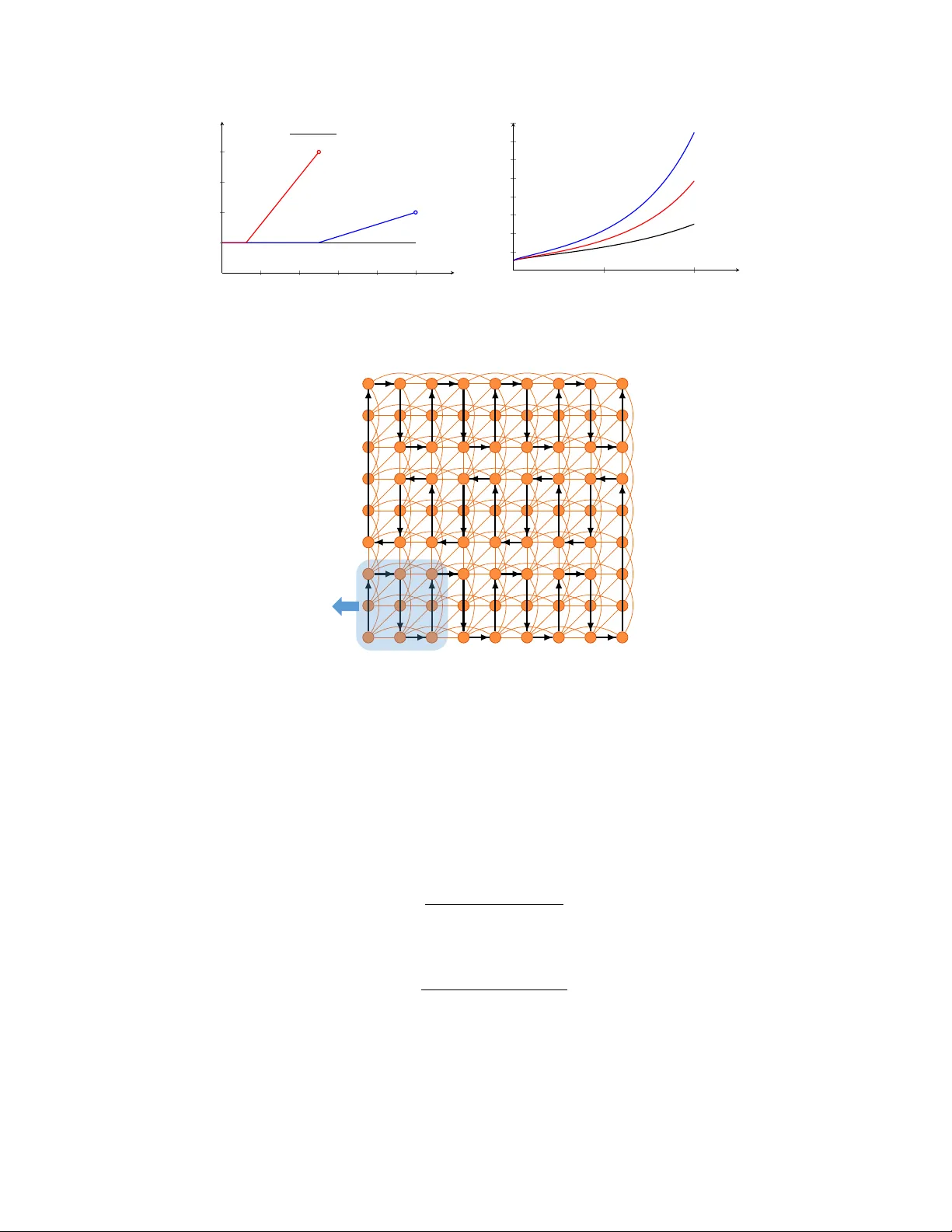
Comm unit y Reco v ery in Graphs with Lo calit y Y uxin Chen ∗ Go vinda Kamath † Changho Suh ‡ Da vid T se § F ebruary 2016; Revised: June 2016 Abstract Motiv ated b y applications in domains such as so cial net works and computational biology , w e study the problem of communit y reco very in graphs with locality . In this problem, pairwise noisy measurements of whether tw o no des are in the same communit y or diﬀerent comm unities come mainly or exclusively from nearb y no des rather than uniformly sampled b et ween all no de pairs, as in most existing mo dels. W e present t wo algorithms that run nearly linearly in the num b er of measurements and which achiev e the information limits for exact recov ery . 1 In tro duction Clustering of data is a central problem that is prev alen t across all of science and engineering. One formu- lation that has received signiﬁcant attention in recent years is communit y recov ery [1–3], also referred to as correlation clustering [4] or graph clustering [5]. In this formulation, the ob jectiv e is to cluster individuals in to diﬀerent comm unities based on pairwise measurements of their relationships, each of whic h gives some noisy information about whether tw o individuals b elong to the same comm unity or diﬀerent comm unities. While this form ulation applies naturally in so cial netw orks, it has a broad range of applications in other domains including protein complex detection [6], image segmen tation [7, 8], shap e matc hing [9], etc. See [10] for an introduction of this topic. In recent years, there has b een a ﬂurry of works on designing communit y reco very algorithms based on idealised generative models of the measuremen t pro cess. A particular p opular mo del is the Sto chastic Blo ck Mo del (SBM) [11, 12], where the n individuals to b e clustered are mo deled as no des on a random graph. In the simplest v ersion of this mo del with tw o communities, this random graph is generated such that tw o no des has an edge connecting them with probability p if they are in the same communit y and probability q if they b elong to diﬀerent communities. If p > q , then there are statistically more edges within a communit y than b et w een tw o communities, which can provide discriminating information for recov ering the communities. A closely related mo del is the Censor e d Blo ck Mo del (CBM) [13], where one obtains noisy parity measuremen ts on the edges of an Erdős-Rén yi graph [14]. Each edge measurement is 0 with probability 1 − θ and 1 with probabilit y θ if the t wo incident vertices are in the same communit y , and vice versa if they are in diﬀerent comm unities. Both the SBM and the CBM can b e uniﬁed in to one mo del b y viewing the measurement process as a t w o-step process. First, the edge lo c ations where there are measurements are determined b y randomly and uniformly sampling a complete graph b et ween the no des. Second, the value of each edge measurement is obtained as a noisy function of the comm unities of the t w o nodes the edge connects. The tw o models diﬀer only in the noisy functions. View ed in this light, it is seen that a cen tral assumption underlying b oth mo dels is that it is equally likely to obtain measuremen ts b et ween any pair of nodes. This is a v ery unrealistic assumption in man y applications: no des often hav e lo c ality and it is more lik ely to obtain data on relationships b et ween nearby no des than far aw a y no des. F or example, in friendship graphs, individuals that liv e close by are more likely to in teract than no des that are far aw a y . ∗ Department of Statistics and of Electrical Engineering, Stanford Universit y , Stanford, CA 94305, USA (email: yx- chen@stanford.edu). † Department of Electrical Engineering, Stanford Universit y , Stanford, CA 94305, USA (email: gk amath@stanford.edu). ‡ Department of Electrical Engineering, KAIST, Daejeon 305-701, Korea (e-mail: chsuh@k aist.ac.kr). § Department of Electrical Engineering, Stanford Universit y , Stanford, CA 94305, USA (email: dntse@stanford.edu). 1 This pap er fo cuses on the comm unity recov ery problem when the measurements are randomly sampled from graphs with lo cality structure rather than complete graphs. Our theory cov ers a broad range of graphs including rings, lines, 2-D grids, and small-world graphs (Fig. 1). Each of these graphs is parametrized by a lo calit y radius r such that no des within r hops are connected b y an edge. W e characterize the informa- tion limits for communit y reco very on these net works, i.e. the minimum n umber of measurements needed to exactly reco ver the communities as the num b er of nodes n scales. W e propose tw o algorithms whose complexities are nearly linear in the num b er of measurements and whic h can achiev e the information limits of all these netw orks for a very wide range of the radius r . In the sp ecial case when the radius r is so large that measurements at all lo cations are p ossible, we recov er the exact recov ery limit identiﬁed by [15] when measuremen ts are randomly sampled from complete graphs. It is worth emphasizing that v arious computationally feasible algorithms [5, 16 – 21] ha ve b een prop osed for more general mo dels beyond the SBM and the CBM, which accommo date m ulti-communit y mo dels, the presence of outlier samples, the case where diﬀeren t edges are sampled at diﬀerent rates, and so on. Most of these models, ho wev er, fall short of accoun ting for an y sort of lo calit y constrain ts. In fact, the results dev elop ed in prior literature often lead to unsatisfactory guarantees when applied to graphs with lo calit y , as will b e detailed in Section 3. Another recent work [22] has determined the order of the information limits in geometric graphs, with no tractable algorithms pro vided therein. In contrast, our ﬁndings uncov er a curious phenomenon: the presence of lo calit y do es not lead to additional computational barriers: solutions that are information theoretically optimal can often b e achiev ed computational eﬃcien tly and, p erhaps more surprisingly , within nearly linear time. The pap er is structured as follows. W e describ e the problem formulation in Section 2, including a concrete application from computational biology—called haplot yp e phasing—which motiv ates m uch of our theory . Section 3 presents our main results, with extensions of the basic theory and numerical results provided in Sections 4 and 5 resp ectiv ely . Section 6 concludes the pap er with a few p otential extensions. The pro ofs of all results are deferred to the app endices. 2 Problem F orm ulation and A Motiv ating Application This section is dev oted to describing a basic mathematical setup of our problem, and to discussing a concrete application that comes from computational biology . 2.1 Sampling Mo del Measuremen t Graph . Consider a collection of n vertices V = { 1 , · · · , n } , eac h represented b y a binary- v alued vertex v ariable X i ∈ { 0 , 1 } , 1 ≤ i ≤ n . Suppose it is only feasible to take pairwise samples ov er a restricted set of lo cations, as represented by a graph G = ( V , E ) that comprises an edge set E . Speciﬁcally , for each edge ( i, j ) ∈ E one acquires N i,j samples 1 Y ( l ) i,j ( 1 ≤ l ≤ N i,j ), where each sample measures the parit y of X i and X j . W e will use G to enco de the lo calit y constraint of the sampling scheme, and shall pay particular atten tion to the following families of measuremen t graphs. • Complete gr aph : G is called a complete graph if every pair of v ertices is connected b y an edge; see Fig. 1(a). • Line : G is said to b e a line L r if, for some lo cality radius r , ( i, j ) ∈ E iﬀ | i − j | ≤ r ; see Fig. 1(b). • Ring : G = ( V , E ) is said to b e a ring R r if, for some locality radius r , ( i, j ) ∈ E iﬀ i − j ∈ [ − r , r ] ( mo d n ); see Fig. 1(c). • Grid : G is called a grid if (1) all v ertices reside within a √ n × √ n square with integer co ordinates, and (2) tw o vertices are connected by an edge if they are at distance not exceeding some radius r ; see Fig. 1(d). • Smal l-world gr aphs : G is said to b e a small-w orld graph if it is a sup erposition of a complete graph G 0 = ( V , E 0 ) and another graph G 1 = ( V , E 1 ) with lo cality . See Fig. 1(e) for an example. 2 | {z } r 1 | {z } r 1 | {z } r 1 | {z } r 1 (a) a complete graph (b) a line L r (c) a ring R r | {z } r 1 | {z } r 1 (d) a grid (e) a small-world graph Figure 1: Examples of a complete graph, a line, a ring, a 2-D grid, and a small-world graph. Random Sampling . This pap er fo cuses on a random sampling mo del, where the num b er of samples N i,j tak en ov er ( i, j ) ∈ E is indep endently drawn and ob eys 2 N i,j ∼ Poisson ( λ ) for some av erage sampling rate λ . This giv es rise to an av erage total sample size m := X ( i,j ) ∈E E [ N i,j ] = λ |E | . (1) When m is large, the actual sample size sharply concentrates around m with high probability . Measuremen t Noise Mo del . The acquired parity measurements are assumed to be indep endent given N i,j ; more precisely , conditional on N i,j , Y ( l ) i,j = Y ( l ) j,i ind. = ( X i ⊕ X j , with probabilit y 1 − θ X i ⊕ X j ⊕ 1 , else (2) for some ﬁxed error rate 0 < θ < 1 , where ⊕ denotes mo dulo-2 addition. This is the same as the noise mo del in CBM [13]. The SBM corresp onds to an asymmetric erasure model for the measurement noise, and w e exp ect our results extend to that mo del as w ell. 2.2 Goal: Optimal Algorithm for Exact Recov ery This paper cen ters on exact recov ery , that is, to reconstruct all input v ariables X = [ X i ] 1 ≤ i ≤ n precisely up to global oﬀset. This is all one can hope for since there is absolutely no basis to distinguish X from X ⊕ 1 := [ X i ⊕ 1] 1 ≤ i ≤ n giv en only parity samples. More precisely , for any reco v ery pro cedure ψ the probabilit y of error is deﬁned as P e ( ψ ) := max X ∈{ 0 , 1 } n P { ψ ( Y ) 6 = X and ψ ( Y ) 6 = X ⊕ 1 } , where Y := { Y ( l ) i,j } . The goal is to develop an algorithm whose required sample complexit y approaches the information limit m ∗ (as a function of ( n, θ ) ), that is, the minimum sample size m under which inf ψ P e ( ψ ) v anishes as n scales. F or notational simplicity , the dep endency of m ∗ on ( n, θ ) shall often b e suppressed when it is clear from the context. 1 Here and throughout, we adopt the conv ention that N i,j ≡ 0 for an y ( i, j ) / ∈ E . 2 All results presen ted in this pap er hold under a related mo del where N i,j ∼ Bernoulli ( λ ) , as long as |E |  n log n and λ ≤ 1 (which is the regime accommo dated in all theorems). In short, this arises due to the tigh tness of Poisson approximation to the Binomial distribution. W e omit the details for conciseness. 3 2.3 Haplot yp e Phasing: A Motiv ating Application Before pro ceeding to present the algorithms, w e describ e here a genome phasing application that motiv ates this researc h and show how it can b e mo deled as a communit y reco very problem on graphs with lo calit y . Humans ha v e 23 pairs of homologous chromosomes, one maternal and one paternal. Eac h pair are iden tical sequences of n ucleotides A,G,C,T’s except on certain do cumen ted p ositions called single nucleotide p olymorphisms (SNPs), or genetic v ariants. At each of these p ositions, one of the chromosomes tak es on one of A,G,C or T which is the same as the ma jority of the p opulation (called the major al lele ), while the other c hromosome takes on a v ariant (also c alled minor al lele ). The problem of haplotype phasing is that of determining which v arian ts are on the same chromosome in each pair, and has imp ortan t applications such as in personalized medicine and understanding p o ylogenetic trees. The adv ent of next generation sequencing tec hnologies allows haplotype phasing by providing linking reads b et w een multiple SNP lo cations [23 – 25]. One can formulate the problem of haplotype phasing as recov ery of tw o communities of SNP lo cations, those with the v ariant on the maternal chromosome and those with the v ariant on the paternal chromosome [26, 27]. Each pair of linking reads giv es a noisy measurement of whether tw o SNPs hav e the v ariant on the same chromosome or diﬀeren t c hromosomes. While there are of the order of n = 10 5 SNPs on each c hromosome, the linking reads are t ypically only sev eral SNPs or at most 100 SNPs apart, dep ending on the sp eciﬁc sequencing technology . Th us, the measurements are sampled from a line graph like in Fig. 1(b) with lo calit y radius r  n . 2.4 Other Useful Metrics and Notation It is con venien t to introduce some notations that will b e used throughout. One key metric that captures the distinguishabilit y b et ween tw o probabilit y measures P 0 and P 1 is the Chernoﬀ information [28], deﬁned as D ∗ ( P 0 , P 1 ) := − inf 0 ≤ τ ≤ 1 log n X y P τ 0 ( y ) P 1 − τ 1 ( y ) o . (3) F or instance, when P 0 ∼ Bernoulli ( θ ) and P 1 ∼ Bernoulli (1 − θ ) , D ∗ simpliﬁes to D ∗ = KL (0 . 5 k θ ) = 0 . 5 log 0 . 5 θ + 0 . 5 log 0 . 5 1 − θ , (4) where KL (0 . 5 k θ ) is the Kullback-Leibler (KL) divergence b et ween Bernoulli (0 . 5) and Bernoulli ( θ ) . Here and b elo w, w e shall use log ( · ) to indicate the natural logarithm. In addition, w e denote by d v and d avg the v ertex degree of v and the av erage vertex degree of G , resp ectiv ely . W e use k M k to represent the sp ectral norm of a matrix M . Let 1 and 0 be the all-one and all-zero vectors, resp ectiv ely . W e denote by supp ( x ) (resp. k x k 0 ) the supp ort (resp. the supp ort size) of x . The standard notion f ( n ) = o ( g ( n )) means lim n →∞ f ( n ) /g ( n ) = 0 ; f ( n ) = ω ( g ( n )) means lim n →∞ g ( n ) /f ( n ) = 0 ; f ( n ) = Ω ( g ( n )) or f ( n ) & g ( n ) mean there exists a constan t c such that f ( n ) ≥ cg ( n ) ; f ( n ) = O ( g ( n )) or f ( n ) . g ( n ) mean there exists a constant c such that f ( n ) ≤ cg ( n ) ; f ( n ) = Θ ( g ( n )) or f ( n )  g ( n ) mean there exist constants c 1 and c 2 suc h that c 1 g ( n ) ≤ f ( n ) ≤ c 2 g ( n ) . 3 Main Results This section describes tw o nearly linear-time algorithms and presents our main results. The pro ofs of all theorems are deferred to the app endices. 3.1 Algorithms 3.1.1 Spectral-Expanding The ﬁrst algorithm, called Sp ectral-Expanding, consists of three stages. F or concreteness, w e start b y describing the procedure when the measurement graphs are lines / rings; see Algorithm 1 for a precise description of the algorithm and Fig. 2 for a graphical illustration. 4 Algorithm 1 : Spectral-Expanding 1. Run sp ectral metho d (Algorithm 2) on a core subgraph induced by V c , whic h yields estimates X (0) j , 1 ≤ j ≤ |V c | . 2. Progressiv e estimation : for i = |V c | + 1 , · · · , n , X (0) i ← majorit y n Y ( l ) i,j ⊕ X (0) j | j : j < i, ( i, j ) ∈ E , 1 ≤ l ≤ N i,j o . 3. Successiv e lo cal reﬁnement: for t = 0 , · · · , T − 1 , X ( t +1) i ← majo rity n Y ( l ) i,j ⊕ X ( t ) j | j : j 6 = i, ( i, j ) ∈ E , 1 ≤ l ≤ N i,j o , 1 ≤ i ≤ n. 4. Output X ( T ) i , 1 ≤ i ≤ n . Here, majo rit y {·} represen ts the ma jorit y v oting rule: for any sequence s 1 , · · · , s k ∈ { 0 , 1 } , majo rity { s 1 , · · · , s k } is equal to 1 if P k i =1 s i > k / 2 ; and 0 otherwise. Algorithm 2 : Spectral initialization 1. Input: measurement graph G = ( V , E ) , and samples n Y ( l ) i,j ∈ { 0 , 1 } | j : j < i, ( i, j ) ∈ E , 1 ≤ l ≤ N i,j o . 2. F orm a sample matrix A such that A i,j = ( 1  Y (1) i,j = 0  − 1  Y (1) i,j = 1  , if ( i, j ) ∈ E ; 0 , else . 3. Compute the leading eigenv ector u of A , and for all 1 ≤ i ≤ n set X (0) i = ( 1 , if u i ≥ 0 , 0 , else . 4. Output X (0) i , 1 ≤ i ≤ n . • Stage 1: sp ectral metro d on a core subgraph . Consider a subgraph G c induced b y V c := { 1 , · · · , r } , and it is self-evident that G c is a complete subgraph. W e run a sp ectral metho d (e.g. [29]) on G c using samples taken ov er G c , in the hop e of obtaining approximate recov ery of { X i | i ∈ V c } . Note that the sp ectral metho d can b e replaced by other eﬃcien t algorithms, including semideﬁnite programming (SDP) [30] and a v ariant of b elief propagation (BP) [31]. • Stage 2: progressive estimation of remaining v ertices. F or each v ertex i > |V c | , compute an estimate of X i b y ma jority v ote using b ackwar d samples —those samples linking i and some j < i . The ob jective is to ensure that a large fraction of estimates obtained in this stage are accurate. As will b e discussed later, the sample complexity required for appro ximate recov ery is m uch low er than that required for exact recov ery , and hence the task is feasible even though we do not use any forw ard samples to estimate X i . • Stage 3: su ccessiv e lo cal reﬁnement. Finally , we clean up all estimates using b oth backw ard and forw ard samples in order to maximize reco very accuracy . This is achiev ed by running lo cal ma jority v oting from the neigh b ors of each v ertex un til conv ergence. In con trast to man y prior w ork, no sample splitting is required, namely , we reuse all samples in all iterations in all stages. As we shall see, this stage is the b ottleneck for exact information recov ery . R emark 1 . The prop osed algorithm falls under the category of a general non-con v ex paradigm, whic h starts 5 V 1 V 2 V 3 V 4 V 5 V 6 core subgraph V c 1 V 1 V 2 V 3 V 4 V 5 V 6 cor e subgr aph V c Stage 1: St a g e 2 : St a g e 3 : St a g es 1 -2 : 1 V 1 V 2 V 3 V 4 V 5 V 6 cor e subgr aph V c St a g e 1 : Stage 2: St a g e 3 : St a g es 1 -2 : 1 V 1 V 2 V 3 V 4 V 5 V 6 cor e subgr aph V c St a g e 1 : St a g e 2 : Stage 3: St a g es 1 -2 : 1 Figure 2: Illustration of the information ﬂo w in Spectral-Expanding: (a) Stage 1 concerns recov ery in a core complete subgraph; (b) Stage 2 makes a forw ard pass by progressively propagating information through bac kward samples; (c) Stage 3 reﬁnes each X v b y employing all samples incident to v . with an approximate estimate (often via sp ectral metho ds) follow ed b y iterative reﬁnemen t. This paradigm has b een successfully applied to a wide sp ectrum of applications ranging from matrix completion [32, 33] to phase retriev al [34] to communit y recov ery [17, 35, 36]. An important feature of this algorithm is its lo w computational complexity . First of all, the sp ectral metho d can b e p erformed within O ( m c log n ) time by means of the p o w er metho d, where m c indicates the n umber of samples falling on G c . Stage 2 entails one round of ma jority voting, whereas the ﬁnal stage—as w e will demonstrate—conv erges within at most O (log n ) rounds of ma jority voting. Note that each round of ma jorit y voting can b e completed in linear time, i.e. in time prop ortional to reading all samples. T aken collectiv ely , we see that Sp ectral-Expanding can b e accomplished within O ( m log n ) ﬂops, which is nearly linear time. Careful readers will recognize that Stages 2-3 bear similarities with BP , and might wonder whether Stage 1 can also be replaced with standard BP . Unfortunately , w e are not aw are of any approac h to analyze the p erformance of v anilla BP without a decent initial guess. Note, how ev er, that the sp ectral metho d is already nearly linear-time, and is hence at least as fast as any feasible pro cedure. While the preceding paradigm is presented for lines / rings, it easily extends to a muc h broader family of graphs with lo cality . The only places that need to b e adjusted are: 1. The core subgraph V c . One w ould like to ensure that |V c | & d avg and that the subgraph G c induced b y V c forms a (nearly) complete subgraph, in order to guarantee decent recov ery in Stage 1. 2. The ordering of the v ertices . Let V c form the ﬁrst |V c | vertices of V , and mak e sure that each i > |V c | is connected to at least an order of d avg v ertices in { 1 , · · · , i − 1 } . This is imp ortan t b ecause eac h vertex needs to be incident to suﬃcien tly man y backw ard samples in order for Stage 2 to b e successful. 3.1.2 Sp ectral-Stitching W e now turn to the 2 nd algorithm called Sp ectral-Stitc hing, which shares similar spirit as Sp ectral-Expanding and, in fact, diﬀers from Sp ectral-Expanding only in Stages 1-2. • Stage 1: no de splitting and sp ectral estimation . Split V into several ov erlapping subsets V l ( l ≥ 1) of size W , such that an y tw o adjacent subsets share W / 2 common vertices. W e choose the size W of each V l to b e r for rings / lines, and on the order of d avg for other graphs. W e then run spectral metho ds separately on each subgraph G l induced by V l , in the hop e of achieving approximate estimates { X V l i | i ∈ V l } —up to global phase—for each subgraph. • Stage 2: stic hing the estimates . The aim of this stage is to stitch together the outputs of Stage 1 computed in isolation for the collection of ov erlapping subgraphs. If approximate recov ery (up to some global phase) has b een achiev ed in Stage 1 for each V l , then the outputs for any tw o adjacent subsets 6 Algorithm 3 : Spectral-Stitching 1. Split all vertices into several (non-disjoint) vertex subsets each of size W as follows V l := { i | ( i − 1) W / 2 + 1 ≤ l ≤ ( i − 1) W / 2 + W } , l = 1 , 2 , · · · , and run spectral method (Algorithm 2) on eac h subgraph induced by V l , whic h yields esti- mates { X V l j | j ∈ V l } for each l ≥ 1 . 2. Stitc hing : set X (0) j ← X V 1 j for all j ∈ V 1 ; for l = 2 , 3 , · · · , X (0) j ← X V l j ( ∀ j ∈ V l ) if X j ∈V l ∩V l − 1 X V l j ⊕ X V l − 1 j ≤ 0 . 5 |V l ∩ V l − 1 | ; and X (0) j ← X V l j ⊕ 1 ( ∀ j ∈ V l ) otherwise . 3. Successiv e lo cal reﬁnement and output X ( T ) i , 1 ≤ i ≤ n (see Steps 3-4 of Algorithm 1). V 1 V 2 V 3 V 4 V 5 V 6 1 V 1 V 2 V 3 V 4 V 5 V 6 1 V 1 V 2 V 3 V 4 V 5 V 6 1 V 1 V 2 V 3 V 4 V 5 V 6 1 V 1 V 2 V 3 V 4 V 5 V 6 1 V 1 V 2 V 3 V 4 V 5 V 6 1 V 1 V 2 V 3 V 4 V 5 V 6 1 V 1 V 2 V 3 V 4 V 5 V 6 1 V 1 V 2 V 3 V 4 V 5 V 6 1 V 1 V 2 V 3 V 4 V 5 V 6 1 V 1 V 2 V 3 V 4 V 5 V 6 1 V 1 V 2 V 3 V 4 V 5 V 6 1 V 1 V 2 V 3 V 4 V 5 V 6 cor e subgr aph V c Stage 1: St a g e 2 : St a g e 3 : St a g es 1 -2 : 1 V 1 V 2 V 3 V 4 V 5 V 6 cor e subgr aph V c St a g e 1 : Stage 2: St a g e 3 : St a g es 1 -2 : 1 V 1 V 2 V 3 V 4 V 5 V 6 cor e subgr aph V c St a g e 1 : St a g e 2 : Stage 3: St a g es 1 -2 : 1 Figure 3: Illustration of the information ﬂow in Sp ectral-Stitc hing: (a) Stage 1 runs sp ectral metho ds for a collection of o verlapping subgraphs of size W separately; (b) Stage 2 stitches all groups of estimates together using the information coming from their ov erlaps; (c) Stage 3 cleans up all estimates by employing all samples inciden t to each no de. are p ositiv ely correlated only when they hav e matching global phases. This simple observ ation allo ws us to calibrate the global phases for all preceding estimates, th us yielding a v ector { X (0) i } 1 ≤ i ≤ n that is appro ximately faithful to the truth mo dulo some global phase. The remaining steps of Sp ectral-Stitc hing follow the same local reﬁnement pro cedure as in Sp ectral- Expanding, and we can employ the same ordering of vertices as in Spectral-Expanding. See Algorithm 3 and Fig. 3. As can b e seen, the ﬁrst 2 stages of Sp ectral-Stitc hing—which can also b e completed in nearly linear time—are more “symmetric” than those of Sp ectral-Expanding. More precisely , Sp ectral-Expanding emphasizes a single core subgraph G c and computes all other estimates based on G c , while Sp ectral-Stitc hing treats eac h subgraph G l almost equiv alently . This symmetry nature might b e practically b eneﬁcial when the acquired data deviate from our assumed random sampling mo del. 3.2 Theoretical Guaran tees: Rings W e start with the p erformance of our algorithms for rings. This class of graphs—which is spatially inv ariant— is arguably the simplest mo del exhibiting lo cality structure. 7 3.2.1 Minimum Sample Complexit y Encouragingly , the proposed algorithms succeed in ac hieving the minimum sample complexit y , as stated b elo w. Theorem 1. Fix θ > 0 and any smal l  > 0 . L et G b e a ring R r with lo c ality r adius r , and supp ose m ≥ (1 +  ) m ∗ , (5) wher e m ∗ = n log n 2  1 − e − KL (0 . 5 k θ )  . (6) Then with pr ob ability appr o aching one 3 , Sp e ctr al-Exp anding (r esp. Sp e ctr al-Stitching) c onver ges to the gr ound truth within T = O (log n ) iter ations, pr ovide d that r & log 3 n (r esp. r ≥ n δ for an arbitr ary c onstant δ > 0 ). Conversely, if m < (1 −  ) m ∗ , then the pr ob ability of err or P e ( ψ ) is appr o aching one for any algorithm ψ . R emark 2 . When r = n − 1 , a ring reduces to a complete graph (or an equiv alent Erdős-Rényi model). F or this case, computationally feasible algorithms hav e b een extensively studied [5, 9, 18, 37, 38], most of which fo cus only on the scaling results. Recen t w ork [15, 39] succeeded in c haracterizing the sharp threshold for this case, and it is immediate to c heck that the sample complexity we derive in (6) matches the one presented in [15, 39]. R emark 3 . Theorem 1 requires r & p oly log( n ) b ecause each no de needs to b e connected to suﬃcien tly man y neighbors in order to preclude “bursty” errors. The condition r & log 3 n migh t b e improv ed to a lo wer-order p oly log ( n ) term using more reﬁned analyses. When r . log n , one can compute the maximum lik eliho o d (ML) estimate via dynamic programming [27] within p olynomial time. Theorem 1 uncov ers a surprising insensitivity phenomenon for rings: as long as the measurement graph is suﬃcien tly connected, the locality constraint do es not alter the sample complexity limit and the com- putational limit at all. This subsumes as special cases tw o regimes that exhibit dramatically diﬀeren t graph structures: (1) complete graphs, where the samples are taken in a global manner, and (2) rings with r = O (poly log ( n )) , where the samples are constrained within highly lo cal neighborho o d. In addition, Theo- rem 1 do es not imp ose an y assumption on the ground truth { X i : 1 ≤ i ≤ n } ; in fact, the success probabilit y of the prop osed algorithms is indep enden t of the true communit y assignment. Notably , b oth [13] and [40] hav e derived general suﬃcien t recov ery conditions of SDP which, ho wev er, dep end on the second-order graphical metrics of G [14] (e.g. the sp ectral gap or Cheeger constant). When applied to rings (or other graphs with lo cality), the suﬃcien t sample complexity giv en therein is signiﬁcan tly larger than the information limit 4 . This is in con trast to our ﬁnding, which reveals that for many graphs with lo calit y , b oth the information and computation limits often dep end only up on the vertex degrees indep enden t of these second-order graphical metrics. 3.2.2 Bottlenecks for Exact Reco very Before explaining the rationale of the prop osed algorithms, w e provide here some heuristic argument as to wh y n log n samples are necessary for exact recov ery and where the recov ery b ottlenec k lies. Without loss of generalit y , assume X = [0 , · · · , 0] > . Supp ose the genie tells us the correct lab els of all no des except v . Then all samples useful for recov ering X v reside on the edges connecting v and its neigh b ors, and there are P oisson ( λd v ) such samples. Th us, this comes do wn to testing b et w een t wo conditionally i.i.d. distributions with a Poisson sample size of mean λd v . F rom the large deviation theory , the ML rule fails in recov ering X v with probabilit y P e ,v ≈ exp n − λd v (1 − e − D ∗ ) o , (7) 3 More precisely , the prop osed algorithms succeed with probability exceeding 1 − c 1 r − 9 − C 2 exp {− c 2 m n (1 − e − D ∗ ) } for some constants c 1 , c 2 , C 2 > 0 . 4 F or instance, the suﬃcien t sample complexit y giv en in [13] scales as n log n h G D ∗ with h G denoting the Cheeger constan t. Since h G = O (1 /n ) for rings / lines, this results in a sample size that is ab out n times larger than the information limit. 8 where D ∗ is the large deviation exp onen t. The ab o ve argument concerns a t ypical error even t for recov ering a single no de v , and it remains to accommo date all vertices. Since the lo cal neigh b orho ods of tw o vertices v and u are nearly non-o verlapping, the resulting typical error ev ents for reco v ering X v and X u b ecome almost indep enden t and disjoin t. As a result, the probability of error of the ML rule ψ ml is appro ximately low er b ounded by P e ( ψ ml ) & X n v =1 P e ,v ≈ n exp n − λd avg (1 − e − D ∗ ) o , (8) where one uses the fact that d v ≡ d avg . Apparently , the right-hand side of (8) would v anish only if λd avg (1 − e − D ∗ ) > log n. (9) Since the total sample size is m = λ · 1 2 nd avg , this together with (9) conﬁrms the sample complexity low er b ound m = 1 2 λnd avg > n log n 2 (1 − e − D ∗ ) = m ∗ . As we shall see, the ab ov e error even ts—in whic h only a single v ariable is uncertain—dictate the hardness of exact recov ery . 3.2.3 Interpretation of Our Algorithms The preceding argument suggests that the reco very b ottlenec k of an optimal algorithm should also b e de- termined by the aforementioned t ypical error even ts. This is the case for b oth Spectral-Expanding and Sp ectral-Stitc hing, as revealed by the intuitiv e arguments b elow. While the intuition is provided for rings, it con tains all imp ortan t ingredients that apply to man y other graphs. T o b egin with, we provide an heuristic argument for Sp ectral-Expanding. (i) Stage 1 fo cuses on a core complete subgraph G c . In the regime where m & n log n , the total num b er of samples falling within G c is on the order of |V c | n · m ≥ |V c | log n , which suﬃces in guaranteeing partial reco very using sp ectral metho ds [29]. In fact, the sample size we hav e av ailable ov er G c is wa y ab o ve the degrees of freedom of the v ariables in G c (whic h is r ). (ii) With decen t initial estimates for G c in place, one can infer the remaining p o ol of vertices one by one using existing estimates together with backw ard samples. One imp ortan t observ ation is that each vertex is incident to many—i.e. ab out the order of log n —backw ard samples. That said, we are eﬀectively op erating in a high signal-to-noise ratio (SNR) regime. While existing estimates are imp erfect, the errors o ccur only to a small fraction of vertices. Moreov er, these errors are in some sense randomly distributed and hence fairly spread out, th us precluding the p ossibilit y of bursty errors. Consequently , one can obtain correct estimate for each of these vertices with high probability , leading to a v anishing fraction of errors in total. (iii) No w that we hav e ac hieved appro ximate reco very , all remaining errors can be cleaned up via lo cal reﬁnemen t using all bac kward and forw ard samples. F or each v ertex, since only a v anishingly small fraction of its neighbors con tain errors, the p erformance of lo cal reﬁnement is almost the same as in the case where all neighbors hav e b een p erfectly recov ered. The ab o ve intuition extends to Spectral-Stitching. F ollowing the argument in (i), w e see that the spe ctral metho d returns nearly accurate estimates for eac h of the subgraph G l induced by V l , except for the global phases (this arises because each G l has b een estimated in isolation, without using any information concerning the global phase). Since any tw o adjacent G l and G l +1 ha ve suﬃcient ov erlaps, this allows us to calibrate the global phases for { X V l i : i ∈ V l } and { X V l +1 i : i ∈ V l +1 } . Once we obtain appro ximate recov ery for all v ariables simultaneously , the remaining errors can then b e cleaned up by Stage 3 as in Sp ectral-Expanding. W e emphasize that the ﬁrst t wo stages of b oth algorithms—whic h aim at appro ximate recov ery—require only O ( n ) samples (as long as the pre-constant is suﬃciently large). In con trast, the ﬁnal stage is the b ottlenec k: it succeeds as long as lo cal reﬁnement for each vertex is successful. The error even ts for this stage are almost equiv alent to the typical even ts singled out in Section 3.2.2, justifying the information- theoretic optimalit y of b oth algorithms. 9 0 . 2 0 . 4 0 . 6 0 . 8 1 1 2 3 4 rings lines grids  ( r = n  ) c  m ⇤ = c · n log n 2(1  e  D ⇤ )  1 0 . 2 0 . 4 0 . 6 0 . 8 1 1 2 3 4 rin gs lin e s grid s  ( r = n  ) c  m ⇤ = c · n log n 2(1  e  D ⇤ )  0 . 1 0 . 2 2 4 6 8 10 12 14 16 L =2 L =3 L !1 error rate: p c  Lm ⇤ = c · n log n  1 Figure 4: (Left) Minim um sample complexit y m ∗ vs. lo calit y radius r ; (Righ t) Minim um n umber Lm ∗ of v ertices b eing measured (including rep etition) vs. single-vertex error rate p . 1 2 3 6 5 4 7 8 9 12 11 10 13 14 15 18 17 16 Community Reco v ery in Graphs with Locality Algorithm 1 1. Run spectral meth od (Algorithm 3 of ( Chin et al. , 2015 )) on a cor e subgraph induced by V c , which yields estimates X (0) j ,1  j  |V c | . 2. Pr ogr essi v e estimation : for i = |V c | + 1, ·· · , n , X (0) i majo ri t y n Y ( l ) i , j  X (0) i | j : j< i ,( i , j ) 2 E ,1  l  N i , j o . 3. Successi v e local r eﬁnement: for t = 0, ·· · , T  1 , X ( t +1 ) i majo ri t y n Y ( l ) i , j  X ( t ) j | j : j 6 = i ,( i , j ) 2 E ,1  l  N i , j o ,1  i  n . 4. Output X ( T ) i , 1  i  n . Here, majo ri t y {· } represents the majority v oting rule: for an y sequence s 1 , ·· · , s k 2 { 0, 1 } , majo ri t y { s 1 , ·· · , s k } is equal to 1 if P k i =1 s i >k / 2 ; and 0 otherwise.    r (a) S tage 1: (b ) S tage 2: (c ) S tage 3: cor e subgr aph V c 1    r (a) S tage 1: (b ) S tage 2: (c ) S tage 3: cor e subgr aph V c 1    r (a) S tage 1: (b ) S tage 2: (c ) S tage 3: cor e subgr aph V c 1    r (a) S tage 1: (b ) S tage 2: (c ) S tage 3: cor e subgr aph G c in s e rt s iz e nu m b e r o f f r a g m e nt s 02 0 0 0 4 0 0 06 0 0 08 0 0 0 1 0 0 0 0 1 Figure 2. Illustration of Algori thm 1 : (a) Stage 1 concerns reco v ery in a core compl ete subgraph; (b) Stage 2 mak es a forw ard pass by progressi v ely propag ating information through backw ard samples; (c) Stage 3 reﬁnes each X v by emplo ying all samples incident to v . approximate reco v ery is much lo wer than that required for e xact reco v ery , and hence the task is feasible e v en though we do not use an y forw ard samples to estimate X i . Stage 3: successi v e local r eﬁnement. Finally , we clean up all estimates using both backw ard and forw ard samples in order to maximize reco v ery accurac y . This is achie v ed by running local majority v oting from the neighbors of each v erte x until con v er gence. As we shall see, this stage is the bottleneck for e xact information reco v ery . Remark 1 . The proposed algorithm f alls under the cate- gory of a general paradigm, which starts with an approx- imate estimate (often via spectral initialization) follo wed by iterati v e reﬁnement. This paradigm has been success- fully applied to a wide spectrum of applications ranging from matrix completion ( K esha v an et al. , 2010a ; Jain et al. , 2013 ) to phase retrie v al ( Candes et al. , 2015 ; Chen & Can- des , 2015 ; Net rapalli et al. , 2013 ) to community reco v- ery ( Chaudhuri et al. , 2012 ; Abbe et al. , 2016 ; Mossel et al. , 2015 ; Gao et al. , 2015 ); see the discussion therein. An important feature of the proposed algorithm is its lo w computational comple xity . First of all, the spectral method can be performed within O ( m c l og n ) time by means of the po wer method, where m c indicates the number of sam- ples f alling on G c . Stage 2 entails one round of majority v oting, whereas the ﬁnal stage—as we will demonstrate— con v er ges within at most O ( l og n ) rounds of majority v ot- ing. Not e that each round of majority v oting can be com- pleted in linear time, i.e. in time proportional to reading all samples. T ak en collecti v ely , we see that Algorithm 1 can be accomplished within O ( m l og n ) ﬂops, which is nearly linear time. Careful readers will recognize that Stages 2-3 share sim- ilarities with BP , and might w onder whether Stage 1 can also be replaced with standard BP . Unfortunately , we are not a w are of an y approach to analyze the performance of v anilla BP without a decent initial guess. Note, ho we v er , that the spectral method is already nearly linear -time, and is hence at least as f ast as an y feasible procedure. While the preceding paradigm is presented for lines / rings, it easily e xtends to a much broader f amily of graphs with locality . The only places that need to be adjusted are: (1) The cor e subgraph V c . One w ould lik e to ensure that |V c | & d av g and that the subgraph G c induced by V c forms a (nearly) complete subgraph, in order to guarantee decent reco v ery in Stage 1. Figure 5: Labeling / ordering of the v ertex set for a grid, where the core subgraph consists of the r 2 v ertices on the b ottom left. 3.3 Theoretical Guaran tees: Inhomogeneous Graphs The prop osed algorithms are guaranteed to succeed for a muc h broader class of graphs with lo calit y b ey ond rings, including those that exhibit inhomogeneous vertex degrees. The follo wing theorem formalizes this claim for tw o of the most imp ortan t instances: lines and grids. Theorem 2. The or em 1 c ontinues to hold for the fol lowing families of me asur ement gr aphs: (1) Lines with r = n β for some c onstant 0 < β < 1 , wher e m ∗ = max { 1 / 2 , β } n log n 1 − e − KL (0 . 5 k θ ) ; (10) (2) Grids with r = n β for some c onstant 0 < β < 0 . 5 , wher e m ∗ = max { 1 / 2 , 4 β } n log n 1 − e − KL (0 . 5 k θ ) . (11) R emark 4 . Note that b oth Spectral-Expanding and Sp ectral-Stitc hing rely on the lab eling / ordering of the v ertex set V . F or lines, it suﬃces to employ the same ordering and core subgraph as for rings. F or grids, w e can start by taking the core subgraph to b e a subsquare of area r 2 lying on the b ottom left of the grid, and then follow a serp en tine tra jectory running alternately from the left to the right and then back again; see Fig. 5 for an illustration. 10 R emark 5 . Careful readers will note that for lines (resp. grids), m ∗ do es not conv erge to n log n 2(1 − e − KL (0 . 5 k θ ) ) as β → 1 (resp. β → 0 . 5 ), whic h is the case of complete graphs. This arises because m ∗ exp eriences a more rapid drop in the regime where β = 1 (resp. β = 0 . 5 ). F or instance, for a line with r = γ n for some constant γ > 0 , one has m ∗ = (1 − γ / 2) n log n 1 − e − KL (0 . 5 k θ ) . Theorem 2 characterizes the eﬀect of lo calit y radius up on the sample complexity limit; see Fig. 4 for a comparison of three classes of graphs. In contrast to rings, lines and grids are spatially v arying mo dels due to the presence of b oundary vertices, and the degree of graph inhomogeneity increases in the lo calit y radius r . T o be more concrete, consider, for example, the ﬁrst d avg / log n v ertices of a line, which hav e degrees around d avg / 2 . In comparison, the set of vertices lying aw ay from the b oundary ha ve degrees as large as d avg . This tells us that the ﬁrst few vertices form a weakly connected comp onen t, thus presenting an additional b ottlenec k for exact recov ery . This issue is negligible unless the size of the w eakly connected comp onen t is exceedingly large. As asserted by Theorem 2, the minimum sample complexity for lines (resp. grids) is iden tical to that for rings unless r & √ n (resp. r & n 1 / 8 ). Note that the curves for lines and grids (Fig. 4) ha ve distinct hinge p oin ts primarily b ecause the vertex degrees of the corresp onding w eakly connected comp onen ts diﬀer. More precisely , the insights developed in Section 3.2.2 readily carry o ver here. Since the error probabilit y of the ML rule is lo wer b ounded by (8), ev erything boils down to determining the smallest λ (called λ ∗ ) satisfying X n v =1 exp n − λ ∗ d v  1 − e − D ∗ o → 0 , whic h in turn yields m ∗ = 1 2 λ ∗ d avg n . The tw o cases accommo dated by Theorem 2 can all b e deriv ed in this w ay . 3.4 Connection to Low-Rank Matrix Completion One can aggregate all correct parities into a matrix Z = [ Z i,j ] 1 ≤ i,j ≤ n suc h that Z i,j = 1 if X i = X j and Z i,j = − 1 otherwise. It is straigh tforw ard to v erify that rank ( Z ) = 1 , with each Y ( l ) i,j b eing a noisy measuremen t of Z i,j . Th us, our problem falls under the category of lo w-rank matrix completion, a topic that has inspired a ﬂurry of research (e.g. [41–45]). Most prior w orks, ho wev er, concen trated on samples tak en ov er an Erdős–RÃ c  n yi mo del, without inv estigating sampling sc hemes with locality constraints. One exception is [46], which explored the eﬀectiveness of SDP under general sampling schemes. How ev er, the sample complexity required therein increases signiﬁcan tly as the sp ectral gap of the measurement graph drops, which do es not deliv er optimal guarantees. W e b eliev e that the approach developed herein will shed ligh t on solving general matrix completion problems from samples with lo cality . 4 Extension: Beyond P airwise Measuremen ts The prop osed algorithms are applicable to numerous scenarios b eyond the basic setup in Section 2.1. This section presen ts tw o imp ortan t extension b eyond pairwise measuremen ts. 4.1 Sampling with Nonuniform W eight In many applications, the sampling rate is non uniform across diﬀeren t edges; for instance, it might fall oﬀ with distance betw een t wo incident vertices. In the haplot yp e phasing application, Fig. 7(a) giv es an example of a distribution of the separation betw een mate-paired reads (insert size). One would naturally w onder whether our algorithm works under this t yp e of more realistic mo dels. More precisely , supp ose the num b er of samples ov er each ( i, j ) ∈ E is indep enden tly generated ob eying N i,j ind ∼ Poisson ( λw i,j ) , (12) where w i,j > 0 incorp orates a sampling rate weigh ting for eac h edge. This section fo cuses on lines / grids / rings for concreteness, where we imp ose the following assumptions in order to make the sampling mo del more “symmetric”: 11 (i) Lines / grids : w i,j dep ends only on the Euclidean distance b etw een vertices i and j ; (ii) R ings : w i,j dep ends only on i − j ( mo d n ). Theorem 3. The or ems 1-2 c ontinue to hold under the ab ove nonuniform sampling mo del, pr ovide d that max ( i,j ) ∈E w i,j min ( i,j ) ∈E w i,j is b ounde d. Theorem 3 might b e surprising at ﬁrst glance: both the p erformance of our algorithms and the funda- men tal limit dep end only on the weigh ted a verage of the v ertex degrees, and are insensitive to the degree distributions. This can b e b etter understo od by examining the three stages of Sp ectral-Expanding and Sp ectral-Stitc hing. T o b egin with, Stages 1-2 are still guaran teed to work gracefully , since we are still op- erating in a high SNR regime irresp ectiv e of the sp eciﬁc v alues of { w i,j } . The main task th us amounts to ensuring the success of lo cal clean-up. Rep eating our heuristic treatment in Section 3.2.2, one sees that the probabilit y of each singleton error even t (i.e. false reco very of X v when the genie already reveals the true lab els of other no des) dep ends only on the av erage n umber of samples incident to each vertex v , namely , E [ N v ] := X j E [ N v ,j ] = X j :( v,j ) ∈E λw v ,j . Due to the symmetry assumptions on { w i } , the total sample size m scales linearly with E [ N v ] , and hence the inﬂuence of { w i } is absorb ed into m and ends up disapp earing from the ﬁnal expression. Another prominen t example is the class of small-w orld graphs. In v arious h uman so cial net works, one t ypically observes b oth lo cal friendships and a (signiﬁcantly lo wer) p ortion of long-range connections, and small-w orld graphs are introduced to incorp orate this feature. T o b etter illustrate the concept, we fo cus on the follo wing spatially-inv arian t instance, but it naturally generalizes to a m uch broader family . • Smal l-world gr aphs . Let G b e a sup erposition of a complete graph G 0 = ( V , E 0 ) and a ring G 1 with connectivit y radius r . The sampling rate is given by N i,j ind. ∼ ( P oisson ( w 0 ) , if ( i, j ) ∈ E 0 ; P oisson ( w 1 ) , else . W e assume that w 0 n 2 w 1 nr = O (1) , in order to ensure higher w eights for lo cal connections. Theorem 4. The or em 1 c ontinues to hold under the ab ove smal l-world gr aph mo del, pr ovide d that r & log 3 n . 4.2 Bey ond Pairwise Measuremen ts In some applications, each measurement ma y co ver more than t wo no des in the graph. In the haplot yp e phasing application, for example, a new sequencing tec hnology called 10x [47] generates barcodes to mark reads from the same chromosome (maternal or paternal), and more than t wo reads can hav e the same barco de. F or concreteness, we supp ose the lo calit y constrain t is captured b y rings, and consider the type of m ultiple linked samples as follows. • Measuremen t (hyper)-graphs . Let G 0 = ( V , E 0 ) b e a ring R r , and let G = ( V , E ) b e a h yp er-graph suc h that (i) every hyper-edge is incident to L vertices in V , and (ii) all these L v ertices are mutually connected in G 0 . • Noise mo del . On each hyper-edge e = ( i 1 , · · · , i L ) ∈ G , we obtain N e ind. ∼ Poisson ( λ ) multi-link ed samples { Y ( l ) e | 1 ≤ l ≤ N e } . Conditional on N e , eac h sample Y ( l ) e is an indep endent copy of Y e = ( ( Z i 1 , · · · , Z i L ) , with prob. 0 . 5 , ( Z i 1 ⊕ 1 , · · · , Z i L ⊕ 1) , else , (13) where Z i is a noisy measurement of X i suc h that Z i = ( X i , with probabilit y 1 − p ; X i ⊕ 1 , otherwise. (14) 12 Here, p represents the error rate for measuring a single vertex. F or the pairwise samples considered b efore, one can think of the parity error rate θ as P { Z i ⊕ Z j 6 = X i ⊕ X j } or, equiv alently , θ = 2 p (1 − p ) . W e emphasize that a random global phase is incorp orated into eac h sample (13). That b eing said, each sample reveals only the r elative similarit y information among these L v ertices, without pro viding further information ab out the absolute cluster mem b ership. Since Algorithm 1 and Algorithm 3 operate only upon pairwise measurements, one alternative is to con vert each L -wise sample Y e = ( Y i 1 , · · · , Y i L ) into  L 2  pairwise samples of the form Y i j ⊕ Y i l (for all j 6 = l ), and then apply the sp ectral metho ds on these parit y samples. In addition, the ma jority voting pro cedure sp eciﬁed in Algorithm 1 needs to b e replaced by certain lo cal maximum likelihoo d rule as well, in order to tak e adv an tage of the mutual data correlation within each L -wise measuremen t. The mo diﬁed algorithms are summarized in Algorithms 4 and 5. In terestingly , these algorithms are still information-theoretically optimal, as asserted by the following theorem. Theorem 5. Fix L ≥ 2 , and c onsider Algorithms 4 and 5 . The or em 1 c ontinues to hold under the ab ove L -wise sampling mo del, with m ∗ r eplac e d by m ∗ := n log n L  1 − e − D ( P 0 ,P 1 )  . Her e, ( P 0 = (1 − p ) Binomial ( L − 1 , p ) + p Binomial ( L − 1 , 1 − p ) ; P 1 = p Binomial ( L − 1 , p ) + (1 − p ) Binomial ( L − 1 , 1 − p ) . (15) Here, the Chernoﬀ information D ( P 0 , P 1 ) can b e expressed in closed form as D ( P 0 , P 1 ) = − log ( L − 1 X i =0  L − 1 i  r n p i (1 − p ) L − i + (1 − p ) i p L − i o n p i +1 (1 − p ) L − i − 1 + (1 − p ) i +1 p L − i − 1 o ) . (16) In particular, when L = 2 , this reduces to 5 D ( P 0 , P 1 ) = KL (0 . 5 k θ ) for θ := 2 p (1 − p ) , which matches our results with pairwise samples. In terestingly , D ( P 0 , P 1 ) enjoys a very simple asymptotic limit as L scales, as stated in the following lemma. Lemma 1. Fix any 0 < p < 1 / 2 . The Chernoﬀ information D ( P 0 , P 1 ) given in The or em 5 ob eys lim L →∞ D ( P 0 , P 1 ) = KL (0 . 5 k p ) . (17) Pr o of. See App endix F.1. R emark 6 . The asymptotic limit (17) admits a simple in terpretation. Consider the typical even t where only X 1 is uncertain and X 2 = · · · = X n = 0 . Conditional on Z 1 , the L − 1 parit y samples ( Z 1 ⊕ Z 2 , · · · , Z 1 ⊕ Z L ) are i.i.d., which reveals accurate information ab out Z 1 ⊕ 0 in the regime where L → ∞ (by the law of large n umber). As a result, the uncertaint y arises only b ecause Z 1 is a noisy version of X 1 , which b eha ves like passing X 1 through a binary symmetric channel with crossov er probability p . This essentially boils down to distinguishing b et ween Bernoulli ( p ) (when X 1 = 0 ) and Bernoulli (1 − p ) (when X 1 = 1 ), for which the asso ciated Chernoﬀ information is kno wn to b e KL (0 . 5 k p ) . With Theorem 5 in place, w e can determine the beneﬁts of multi-link ed sampling. T o enable a fair comparison, we ev aluate the sampling eﬃciency in terms of Lm ∗ rather than m ∗ , since Lm ∗ captures the total num b er of vertices (including rep etition) one needs to measure. As illustrated in Fig. 4, the sampling eﬃciency impro ves as L increases, but there exists a fundamental low er barrier given by n log n 1 − e − KL (0 . 5 k p ) . This lo wer barrier, as plotted in the blac k curve of Fig. 4, corresp onds to the case where L is approac hing inﬁnit y . 5 This follows since, when L = 2 , D ( P 0 , P 1 ) = − log  2 q ((1 − p ) 2 + p 2 ) (2 p (1 − p ))  = − log n 2 p (1 − θ ) θ o = KL (0 . 5 k θ ) . 13 Algorithm 4 : Sp ectral-Expanding for m ulti-linked samples 1. Break eac h L -wise sample Y e = ( Y i 1 , · · · , Y i L ) into  L 2  pairwise samples of the form Y i j ⊕ Y i l (for all j 6 = l ), and run sp ectral metho d (Algorithm 2) on a core subgraph induced by V c using these parit y samples. This yields estimates X (0) j , 1 ≤ j ≤ |V c | . 2. Progressiv e estimation : for k = |V c | + 1 , · · · , n , X (0) k ← lo cal − ML n X (0) i | 1 ≤ i 2 comm unities, whic h naturally arises in many applications including haplot yp e phasing for p olyploid species [50]. F urthermore, what would be the information and computation limits in the regime where the n umber M of comm unities scales with n ? In fact, there often exists a computational barrier aw ay from the information limit when the measuremen t graph is drawn from the Erdős-Rén yi mo del for large M (e.g. [51]). Ho w will this computational barrier b e inﬂuenced b y the lo calit y structure of the measurement graph? In addition, the present theory op erates under the assumption that L is a ﬁxed constan t, namely , each m ulti-linked measurement en tails only a small n umber of samples. Will the prop osed algorithms still b e optimal if L is so large that it has to scale with n ? More broadly , it remains to develop a uniﬁed and systematic approach to accommo date a broader family of graphs b ey ond the instances considered herein. In particular, what would be an optimal recov ery scheme if the graph is far from spatially-in v ariant or if there exist a few fragile cuts? Finally , as mentioned b efore, it w ould b e interesting to see how to develop more general low-rank matrix completion paradigms, when the rev ealed entries come from a sampling pattern that exhibits lo cality structure. 17 A Preliminaries Before contin uing to the proofs, we gather a few facts that will be useful throughout. First of all, recall that the maxim um likelihoo d (ML) decision rule achiev es the lo west Ba yesian probability of error, assuming uniform prior ov er tw o hypotheses of interest. The resulting error exp onent is determined by the Chernoﬀ information, as given in the following lemma. Lemma 2. Fix any  > 0 . Supp ose we observe a c ol le ction of N z r andom variables Z = { Z 1 , · · · , Z N z } that ar e i.i.d. given N z . Consider two hyp otheses H 0 : Z i ∼ P 0 and H 1 : Z i ∼ P 1 for two given pr ob ability me asur es P 0 and P 1 . Assume that the Chernoﬀ information D ∗ = D ( P 0 , P 1 ) > 0 and the alphab et of Z i ar e b oth ﬁnite and ﬁxe d, and that max z P 1 ( z ) P 0 ( z ) < ∞ . (a) Conditional on N z , one has exp {− (1 +  ) N z D ∗ } ≤ P 0  P 1 ( Z ) P 0 ( Z ) ≥ 1     N z  ≤ exp {− N z D ∗ } , (18) wher e the lower b ound holds when N z is suﬃciently lar ge. (b) If N z ∼ Poisson ( N ) , then exp n − (1 +  ) N  1 − e − D ∗ o ≤ P 0  P 1 ( Z ) P 0 ( Z ) ≥ 1  ≤ exp n − N  1 − e − D ∗ o , (19) wher e the lower b ound holds when N is suﬃciently lar ge. Pr o of. See App endix F.2. W e emphasize that the b est achiev able error exp onen t coincides with the Chernoﬀ information D ∗ when the sample size is ﬁxed, while it b ecomes 1 − e − D ∗ —whic h is sometimes termed the Chernoﬀ-Hellinger div ergence—when the sample size is Poisson distributed. The next result explores the robustness of the ML test. In particular, w e control the probability of error when the ML decision b oundary is slightly shifted, as stated b elo w. Lemma 3. Consider any  > 0 , and let N ∼ P oisson ( λ ) . (a) Fix any 0 < θ < 0 . 5 . Conditional on N , dr aw N indep endent samples Z 1 , · · · , Z N such that Z i ∼ Bernoulli ( θ ) , 1 ≤ i ≤ N . Then one has P ( N X i =1 Z i ≥ 1 2 N − λ ) ≤ exp   · 2 log 1 − θ θ λ  exp n − λ  1 − e − KL (0 . 5 k θ ) o . (20) (b) L et P 0 and P 1 b e two distributions ob eying max z P 1 ( z ) P 0 ( z ) < ∞ . Conditional on N , dr aw N indep endent samples Z i ∼ P 0 , 1 ≤ i ≤ N . Then one has P 0    N X j =1 log P 1 ( Z i ) P 0 ( Z i ) ≥ − λ    ≤ exp ( λ ) exp n − λ  1 − e − D ∗ o , (21) wher e D ∗ = D ( P 0 , P 1 ) denotes the Chernoﬀ information b etwe en P 0 and P 1 . Pr o of. See App endix F.3. F urther, the following lemma develops an upp er b ound on the tail of Poisson random v ariables. Lemma 4. Supp ose that N ∼ P oisson ( λ ) for some 0 <  < 1 . Then for any c 1 > 2 e , one has P  N ≥ c 1 λ log 1   ≤ 2 exp  − c 1 λ 2  . Pr o of. See App endix F.4. 18 A dditionally , our analysis relies on the w ell-known Chernoﬀ-Ho eﬀding inequalit y [52, Theorem 1, Eqn (2.1)]. Lemma 5 ( Chernoﬀ-Hoeﬀding Inequality ) . Supp ose Z 1 , · · · , Z n ar e indep endent Bernoul li r andom variables with me an E [ Z i ] ≤ p . Then for any 1 > q ≥ p , one has P  1 n X n j =1 Z j ≥ q  ≤ exp {− n KL ( q k p ) } , wher e KL ( q k p ) := q log q p + (1 − q ) log 1 − q 1 − p . W e end this section with a lo wer b ound on the KL divergence b et ween tw o Bernoulli distributions. F act 1. F or any 0 ≤ q ≤ τ ≤ 1 , KL ( τ k q ) := τ log τ q + (1 − τ ) log 1 − τ 1 − q ≥ τ log ( τ /q ) − τ . Pr o of. By deﬁnition, KL ( τ k q ) ( i ) ≥ τ log τ q + (1 − τ ) log (1 − τ ) ( ii ) ≥ τ log ( τ /q ) − τ , where (i) follows since log 1 1 − q ≥ 0 , and (ii) arises since (1 − τ ) log (1 − τ ) ≥ − (1 − τ ) τ ≥ − τ . B P erformance Guaran tees of Sp ectral-Expanding The analyses for all the cases follow almost identical argumen ts. In what follows, we separate the proofs in to t wo parts: (1) the optimality of Spectral-Expanding and Sp ectral-Stitc hing, and (2) the minimax low er b ound, where each part accommo dates all mo dels studied in this work. W e start with the p erformance guarantee of Sp ectral-Expanding in this section. Without loss of generality , w e will assume X 1 = · · · = X n = 0 throughout this section. F or simplicity of presentation, we will fo cus on the most c hallenging b oundary case where m  n log n , but all arguments easily extend to the regime where m  n log n . B.1 Stage 1 gives appro ximate reco very for G c This subsection demonstrates that the sp ectral metho d (Algorithm 2) is successful in recov ering a p ortion 1 − o (1) of the v ariables in V c with high probability , as stated in the follo wing lemma. Lemma 6. Fix θ > 0 . Supp ose that G = ( V , E ) is a c omplete gr aph and the sample size m & n log n . The estimate X (0) = h X (0) i i 1 ≤ i ≤ n r eturne d by Algorithm 2 ob eys min n k X (0) − X k 0 , k X (0) + X k 0 o = o ( n ) (22) with pr ob ability exc e e ding 1 − O  n − 10  . Pr o of. See App endix F.6. R emark 7 . Here, 1 − O  n − 10  can b e replaced by 1 − O ( n − c ) for any other p ositiv e constant c > 0 . R emark 8 . It has been shown in [29, Theorem 1.6] that a truncated v ersion of the sp ectral method returns reasonably go od estimates ev en in the sparse regime (i.e. m  n ). Note that truncation is in tro duced in [29, Theorem 1.6] to cop e with the situation in whic h some ro ws of the sample matrix are “ov er-represented”. This b ecomes unnecessary in the regime where m & n log n , since the num b er of samples incident to eac h v ertex concentrates around Θ (log n ) , thus precluding the existence of “ov er-represen ted” ro ws. 19 A ccording to Lemma 6, Stage 1 accurately recov ers (1 − o (1)) |V c | v ariables in V c mo dulo some global phase, as long as λ |V c | 2 & |V c | · log n. Since λ  m/n 2 and |V c |  d avg , this condition is equiv alent to m & n log n, whic h falls within our regime of interest. Throughout the rest of the section, we will assume without loss of generalit y that 1 |V c | V c X i =1 1 n X (0) i 6 = X i o = o (1) , i.e. the ﬁrst stage obtains approximate recov ery along with the correct global phase. B.2 Stage 2 yields appro ximate recov ery for V \V c F or concreteness, we start by establishing the achiev ability for lines and rings, which already contain all imp ortan t ingredien ts for proving the more general cases. B.2.1 Lines / rings W e divide all vertices in V \V c in to small groups {V i } , eac h consisting of  log 3 n adjacen t vertices 6 : V i :=  |V c | + ( i − 1)  log 3 n + 1 , · · · , |V c | + i ·  log 3 n  , where  > 0 is some arbitrarily small constan t. In what follo ws, we will con trol the estimation errors happ ening within each group. F or notational simplicity , we let V 0 := V c . An imp ortant vertex set for the progressiv e step, denoted by V → i , is the one encompassing all vertices preceding and connected to V i ; see Fig. 9 for an illustration. The pro of is recursiv e, whic h mainly consists in establishing the claim below. T o state the claim, we need to in tro duce a collection of even ts as follo ws A 0 := n at most a fraction  2 of progressiv e estimates n X (0) j : j ∈ V c o is incorrect o ; A i := n at most a fraction  of progressive estimates n X (0) j : j ∈ V i o is incorrect o , i ≥ 1 . Lemma 7. F or any i ≥ 0 , c onditional on A 0 ∩ · · · ∩ A i , one has P {A i +1 | A 0 ∩ · · · ∩ A i } ≥ 1 − O  n − 10  . (23) As a r esult, one has P {∩ i ≥ 0 A i } ≥ 1 − O  n − 9  . (24) Apparen tly , A 0 holds with high probabilit y; see the analysis for Stage 1. Th us, if (23) holds, then (24) follo ws immediately from the union bound. In fact, (24) suggests that for an y group V i , only a small fraction of estimates obtained in this stage w ould b e incorrect, thus justifying appro ximate recov ery for this stage. Moreo ver, since the neighborho od N ( v ) of eac h no de v ∈ V i is co vered by at most O  d avg |V i |  groups, the even t ∩ i ≥ 0 A i immediately suggests that there are no more than O (  · |V i | ) O  d avg |V i |  = O ( d avg ) errors o ccurring to either the neighborho o d N ( v ) or the backw ard neigh b orhoo d N ( v ) ∩ V → i . This observ ation will prov e useful for analyzing Stage 3, and hence we summarize it in the follo wing lemma. 6 Note that the errors o ccurring to distinct vertices are statistically dep enden t in the progressive estimation stage. The approach we prop ose is to lo ok at a group of vertices simultaneously , and to b ound the fraction of errors happ ening within this group. In order to exhibit suﬃciently sharp concentration, we pick the group size to b e at least  log 3 n . A smaller group is possible via more reﬁned arguments. 20 | {z } V i V ! i V i  1 V i  2 1 | {z } V i V ! i V i  1 V i  2 1 | {z } V i V ! i V i  1 V i  2 1 | {z } V i V ! i V i  1 V i  2 1 | {z } V i V ! i V i  1 V i  2 1 | {z } V i V ! i V i  1 V i  2 1 | {z } V i V ! i V i  1 V i  2 1 | {z } V i V ! i V i  1 V i  2 1 u (a) X X X X ⇥ u | {z } V i V ! i V i  1 V i  2 1 | {z } V i V ! i V i  1 V i  2 1 | {z } V i V ! i V i  1 V i  2 1 | {z } V i V ! i V i  1 V i  2 1 (b) Figure 9: (a) Illustration of V i , V → i , and B u , where B u is the set of samples lying on the dark blue edges. (b) Illustration of B goo d u and B bad u , whic h correspond to the set of samples lying on the set of blue edges and black edges, resp ectiv ely . Here, the symbol X (resp. × ) indicates that the asso ciated no de has b een estimated correctly (resp. incorrectly). Lemma 8. Ther e ar e at most O ( d avg ) err ors o c curring to either the neighb orho o d N ( v ) or the b ackwar d neighb orho o d N ( v ) ∩ V → i . The rest of the section is devoted to establish the claim (23) in Lemma 7. Pr o of of L emma 7 . As discussed ab o ve, it suﬃces to prov e (23) (which in turn justiﬁes (24)). The fol- lo wing argument is conditional on A 0 ∩ · · · ∩ A i and all estimates for V 0 ∪ · · · ∪ V i ; w e shall suppress the notation b y dropping this conditional dep endence whenever it is clear from the con text. Consider an y vertex u ∈ V i +1 . In the progressive estimation step, each X (0) u relies on the preceding estimates n X (0) j | j : j < u, ( j, u ) ∈ E o , as well as the set B u of bac kward samples incident to u , that is, B u := n Y ( l ) u,j | j < u, ( j, u ) ∈ E , 1 ≤ l ≤ N u,j o ; see Fig. 9(a). W e divide B u in to tw o parts • B goo d u : the set of samples Y ( l ) u,j in B u suc h that (i) X (0) j = X j , and (ii) j ∈ V → ( i +1) ; • B bad u : the remaining samples B u \B goo d u ; and set N goo d u :=   B goo d u   and N bad u :=   B bad u   . In words, B goo d u is asso ciated with those preceding estimates in V → ( i +1) that are consistent with the truth, while B bad u en tails the rest of the samples that might b e unreliable. See Fig. 9(b) for an illustration. The purp ose of this partition is to separate out B bad u , whic h only accounts for a small fraction of all samples. W e no w pro ceed to analyze the ma jorit y v oting pro cedure which, by deﬁnition, succeeds if the total votes fa voring the truth exceeds 1 2  N goo d u + N bad u  . T o preclude the eﬀect of B bad u , we pay particular attention to the part of votes obtained ov er B goo d u ; that is, the partial score score goo d u := X Y ( l ) u,j ∈B goo d u X (0) j ⊕ Y ( l ) u,j . It is self-evident to chec k that the ab o v e success condition would hold if score goo d u < 1 2  N goo d u + N bad u  −   B bad u   = 1 2 N goo d u − 1 2 N bad u , 21 and w e further deﬁne the complement even t as D u :=  score goo d u ≥ 1 2 N goo d u − 1 2 N bad u  . The main p oint to work with D u is that conditional on all prior estimates in V → ( i +1) , the D u ’s are indep endent across all u ∈ V i +1 . W e claim that P {D u } = exp {− Θ (log n ) } := P e , 1 . (25) If this claim holds, then w e can con trol the num b er of incorrect estimates within the group V i +1 via the Chernoﬀ-Ho eﬀding inequality . Sp eciﬁcally , P    1  log 3 n X u ∈V i +1 1 n X (0) u 6 = X u o ≥ 1 log 2 n    ≤ P    1  log 3 n X u ∈V i +1 1 {D u } ≥ 1 log 2 n    ( a ) ≤ exp  −  log 3 n · KL  1 log 2 n     E [ 1 {D u } ]  ≤ exp  −  log 3 n · KL  1 log 2 n     P e , 1  ( b ) ≤ exp  −  log 3 n · 1 log 2 n  log 1 P e , 1 log 2 n − 1  ( c ) = exp  − Θ   log 2 n  < O  1 n 10  , where (a) follows from Lemma 5, (b) arises from F act 1, and (c) is a consequence of (25). This reveals that the fraction of incorrect estimates for V i is v anishingly small with high probabilit y , thus establishing the claim (23). Finally , it remains to prov e (25). T o this end, we decouple D u in to tw o ev ents: P {D u } ≤ P  N bad u ≥ c 0 log n log 1   + P  score goo d u ≥ 1 2 N true u − 1 2 c 0 log n log 1   (26) for some universal constant c 0 > 0 . Recall that each edge is sampled at a P oisson rate λ  m |E 0 |  n log n nd avg  log n d avg , and that the av erage num b er of samples connecting u and other no des in V i +1 is atmost λ · O ( d avg ) (recalling our assumption that r & log 3 n ). On the ev en t A 0 ∩ · · · ∩ A i , the n umber of wrong labels in V → ( i +1) is O ( d u ) , and hence E  N bad u  ≤ O ( λd u ) ≤ c 2 log n (27) for some constant c 2 > 0 . This further gives E  N goo d u  ≥ λc 3 d u − E  N bad u  ≥ (1 − c 4  ) c 3 λd u for some constants c 3 , c 4 > 0 . Thus, Lemma 4 and the inequality (27) tak en collectively yield P  N bad u ≥ c 1 c 2 log n log 1   ≤ 2 exp  − c 1 c 2 log n 2  for an y c 1 > 2 e . In addition, in view of Lemma 3, there exists some function ˜ ξ ( · ) suc h that P  score goo d u ≥ 1 2 N true u − 1 2 c 0 log n log 1   ≤ exp n − (1 − o n (1))  1 − ˜ ξ (  )  c 3 λd u  1 − e − D ∗ o = exp {− Θ (log n ) } , 22 where ˜ ξ (  ) is indep enden t of n and v anishes as  → 0 . Putting these b ounds together reveals that: when λ  log n d avg and c 0 = c 1 c 2 , there exists some function ˆ ξ (  ) indep enden t of n such that (26) ≤ 2 exp  − c 1 c 2 log n 2  + exp  − (1 − o n (1))  1 − ˜ ξ (  )  λd avg 2  1 − e − D ∗   = exp {− Θ (log n ) } := P e , 1 , (28) where ˆ ξ (  ) v anishes as  → 0 . This ﬁnishes the pro of. B.2.2 Beyond lines / rings The preceding analysis only relies on very few properties of lines / rings, and can b e readily applied to man y other graphs. In fact, all arguments contin ue to hold as long as the following assumptions are satisﬁed: 1. In G , each vertex v ( v > |V c | ) is connected with at least Θ( d avg ) vertices in { 1 , · · · , v − 1 } by an edge; 2. F or an y v ∈ V i ( i ≥ 1 ), its b ackwar d neighborho o d N ( v ) ∩ V → i is co vered by at most O  d avg |V i |  = O  d avg  log 3 n  distinct groups among V 1 , · · · , V i − 1 . In short, the ﬁrst condition ensures that the information of a diverse range of prior vertices can b e propagated to each v , whereas the second condition guarantees that the estimation errors are fairly spread out within the bac kward neighborho od asso ciated with eac h no de. W e are now in p osition to lo ok at grids, small-world graphs, as well as lines / rings with non uniform w eights. (a) It is straigh tforward to v erify that the c hoices of V c and the ordering of V suggested in Section 3.3 satisfy Conditions 1-2, thus establishing approximate recov ery for grids. (b) Supp ose max ( i,j ) ∈E w i,j min ( i,j ) ∈E w i,j is b ounded. Deﬁne the weigh ted degree as d w v := X i :( i,v ) ∈E w i,v and let the a verage weigh ted degree b e d w avg := 1 n P d w v . Then all argumen ts contin ue to hold if d v and d avg are replaced by d w v and d w avg , resp ectiv ely . This reveals appro ximate recov ery for lines / rings / grids under sampling with nonuniform weigh t. (c) The pro of for small-world graphs follo ws exactly the same argument as for rings. (d) F or the case with multi-link ed samples, we redeﬁne several metrics as follows: – B u : the set of bac kward samples n Y ( l ) e | u ∈ e, j < u for all other j ∈ e, 1 ≤ l ≤ N e o , where e represen ts the hyper-edge; – B goo d u : the set of samples Y ( l ) e in B u suc h that (i) X (0) j = X j for all j ∈ e and j 6 = u , and (ii) j ∈ V → ( i +1) for all j ∈ e and j 6 = u ; – B bad u : the remaining samples B u \B goo d u . – W e also need to re-deﬁne the score score goo d u as score goo d u := X Y ( l ) e ∈B goo d u log P n Y ( l ) e | X u = 1 , X i = X (0) i ( i ∈ e, i 6 = u ) o P n Y ( l ) e | X u = 0 , X i = X (0) i ( i ∈ e, i 6 = u ) o with the decision b oundary replaced b y 0 and the even t D u replaced b y D u :=  score goo d u ≥ 0 − s max · |B bad u |  =  score goo d u ≥ − s max N bad u  . 23 Here, s max indicates the maximum p ossible lik eliho o d ratio for each L -wise sample: s max := max Y e , { Z i }     log P { Y e | X u = 1 , X i = Z i ( i ∈ e, i 6 = u ) } P { Y e | X u = 0 , X i = Z i ( i ∈ e, i 6 = u ) }     . With these metrics in place, all proof arguments for the basic setup carry o v er to the m ulti-linked sample case. B.3 Stage 3 achiev es exact reco very W e now turn to the last stage, and the goal is to prov e that X ( t ) con verges to X within O (log n ) iterations. Before pro ceeding, we introduce a few more notations that will b e used throughout. • F or any vertex v , denote b y N ( v ) the neighb orho o d of v in G , and let S ( v ) b e the set of samples that in volv e v ; • F or any vector Z = [ Z 1 , · · · , Z n ] > and any set I ⊆ { 1 , · · · , n } , deﬁne the ` 0 norm restricted to I as follo ws k Z k 0 , I := X i ∈I 1 { Z i 6 = 0 } . • Generalize the deﬁnition of the ma jorit y vote op erator such that majo rity ( Z ) = [ majorit y 1 ( Z 1 ) , · · · , majo rity n ( Z n )] > obtained b y applying majorit y v ( · ) comp onen t-wise, where majo rity v ( Z v ) := ( 1 , if Z v ≥ 1 2 |S ( v ) | ; 0 , else . • Let V Z (resp. V X ) denote the lo cal voting scores using Z = [ Z i ] 1 ≤ i ≤ n (resp. X = [ X i ] 1 ≤ i ≤ n = 0 ) as the curren t estimates, i.e. for any 1 ≤ u ≤ n , ( V Z ) u = X Y ( l ) i,u ∈S ( u ) Y ( l ) i,u ⊕ Z i ; (29) ( V X ) u = X Y ( l ) i,u ∈S ( u ) Y ( l ) i,u ⊕ X i = X y ( l ) i,u ∈S ( u ) Y ( l ) i,u . (30) With these notations in place, the iterative pro cedure can b e succinctly written as X ( t +1) = majo rity ( V X ( t ) ) . The main sub ject of this section is to prov e the following theorem. Theorem 6. Consider any 0 <  ≤  0 , wher e  0 is some suﬃciently smal l c onstant. Deﬁne Z  := n Z ∈ { 0 , 1 } n | ∀ v : k Z − X k 0 , N ( v ) ≤ d v o . (31) Then with pr ob ability appr o aching one, majo rity ( V Z ) ∈ Z 1 2  , ∀ Z ∈ Z  and ∀  ∈  1 d max ,  0  . R emark 9 . When the iterate falls within the set Z  (cf. (31)), there exist only a small n umber of errors o ccurring to the neigh b orho od of each vertex. This essen tially implies that (i) the fraction of estimation errors is low; (ii) the estimation errors are fairly spread out instead of clustering within the neighborho ods of a few no des. 24 R emark 10 . This is a uniform result: it holds regardless of whether Z is statistically indep enden t of the samples Y or not. This diﬀers from many prior results (e.g. [17]) that emplo y fresh samples in each stage in order to decouple the statistical dep endency . Note that the subscript of Z  indicates the fraction of estimation errors allow ed in an iterate. A ccording to the analyses for the the preceding stages, Stage 3 is seeded with some initial guess X (0) ∈ Z  for some arbitrarily small constan t  > 0 . This taken collectively with Theorem 6 gives rise to the follo wing error con traction result: for any t ≥ 0 , k X ( t +1) − X k 0 , N ( v ) = k majo rity ( V X ( t ) ) − X k 0 , N ( v ) ≤ 1 2 k X ( t ) − X k 0 , N ( v ) , 1 ≤ v ≤ n. (32) This rev eals the geometric con vergence rate of X ( t ) , namely , X ( t ) con verges to the truth within O (log n ) iterations, as claimed. The rest of this section is devoted to proving Theorem 6. W e will start b y proving the result for an y ﬁxed candidate Z ∈ Z  indep enden t of the samples, and then generalize to simultaneously accommodate all Z ∈ Z  . Our strategy is to ﬁrst quantify V X (whic h corresp onds to the score we obtain when only a single v ertex is uncertain), and then con trol the diﬀerence b et ween V X and V Z . W e make the observ ation that all en tries of V X are strictly b elow the decision b oundary , as asserted by the following lemma. Lemma 9. Fix any smal l c onstant δ > 0 , and supp ose that m  n log n . Then one has ( V X ) u < 1 2 |S ( u ) | − δ log n = 1 2 |S ( u ) | − δ · O ( λd u ) , 1 ≤ u ≤ n with pr ob ability exc e e ding 1 − C 1 exp  − c 1 m n  1 − e − D ∗  for some c onstants C 1 , c 1 > 0 , pr ovide d that the fol lowing c onditions ar e satisﬁe d: (1) Rings with r & log 2 n : m >  1 + ξ ( δ )  n log n 2  1 − e − KL (0 . 5 k θ )  ; (2) Lines with r = n β for some c onstant 0 < β < 1 : m >  1 + ξ ( δ )  max  β , 1 2  n log n 1 − e − KL (0 . 5 k θ ) ; (3) Lines with r = γ n for some c onstant 0 < γ ≤ 1 : m >  1 + ξ ( δ )   1 − 1 2 γ  n log n 1 − e − KL (0 . 5 k θ ) ; (4) Grids with r = n β for some c onstant 0 < β < 1 / 2 : m >  1 + ξ ( δ )  max  4 β , 1 2  n log n 1 − e − KL (0 . 5 k θ ) ; (5) Smal l-world gr aphs: m >  1 + ξ ( δ )  n log n 2  1 − e − KL (0 . 5 k θ )  ; In al l these c ases, ξ ( · ) is some function indep endent of n satisfying ξ ( δ ) → 0 as δ → 0 . Her e, we al low Cases (1), (2) and (4) to have nonuniform sampling weight over diﬀer ent e dges, as long as max ( i,j ) ∈E w i,j min ( i,j ) ∈E w i,j is b ounde d. Pr o of. See App endix F.7. It remains to control the diﬀerence b et ween V X and V Z : ∆ Z := V Z − V X . 25 Sp eciﬁcally , we w ould like to demonstrate that most en tries of ∆ Z are b ounded in magnitude by δ log n (or δ · O ( λd u ) ), so that most of the p erturbations are absolutely controlled. T o facilitate analysis, we decouple the statistical dep endency by writing V Z = F Z + B Z , where F Z represen ts the votes using only forward samples, namely , ( F Z ) u = X i>u, Y ( l ) i,u ∈S ( u ) Y ( l ) i,u ⊕ Z i , 1 ≤ u ≤ n. This is more conv enient to work with since the entries of F Z (or B Z ) are jointly indep enden t. In what follo ws, w e will fo cus on b ounding F Z , but all argumen ts immediately apply to B Z . T o simplify presentation, we also decomp ose V X in to tw o parts V X = F X + B X in the same manner. Note that the v th entry of the diﬀerence ∆ F := F Z − F X (33) is generated by those en tries from indices in N ( v ) satisfying Z v 6 = X v . F rom the assumption (31), eac h ∆ F v (1 ≤ v ≤ n ) is dependent on at most O ( d v ) non-zero entries of Z − X , and hence on av erage each ∆ F v is only aﬀected by O ( λ · d avg ) samples. Moreo ver, eac h non-zero entry of Z − X is b ounded in magnitude by a constan t. This together with Lemma 4 yields that: for any suﬃciently large constan t c 1 > 0 , P    ∆ F i   ≥ c 1 λd avg log 1   ≤ 2 exp {− Θ ( c 1 λd avg ) } ≤ 2 n − c 2 , (34) pro vided that λd avg & log n (which is the regime of interest), where c 2 = Θ ( c 1 ) is some absolute p ositiv e constan t. In fact, for any index i , if   ∆ F i   ≥ c 1 λd avg log 1  , then picking suﬃciently small  > 0 w e hav e   ∆ F i    λd avg of   ∆ F i    log n, and hence ( F Z ) i and ( F X ) i b ecome suﬃciently close. The preceding b ound only concerns a single comp onen t. In order to obtain ov erall control, w e in tro duce a set of indep endent indicator v ariables { η i ( Z ) } : η i ( Z ) := ( 1 , if   ∆ F i   ≥ c 1 λd avg log(1 / ) , 0 , else . F or any 1 ≤ v ≤ n , applying Lemma 5 gives P    1 d v X i ∈N ( v ) η i ( Z ) ≥ τ    ≤ exp n − d v KL  τ k max i E [ η i ( Z )] o ≤ exp n − d v  τ log τ 2 n − c 2 − τ o , where the last line follows from F act 1 as well as (34). F or any τ ≥ 1 /n , τ log τ 2 n − c 2 − τ & τ log n, indicating that P    1 d v X i ∈N ( v ) η i ( Z ) ≥ τ    ≤ exp {− c 3 τ d avg log n } for some univ ersal constant c 3 > 0 . If we pick  > 0 and τ > 0 to b e suﬃcien tly small, we see that with high probabilit y most of the entries hav e   ∆ F i   < c 1 λd avg log 1   λd avg . 26 W e are no w in p osition to derive the results in a more uniform fashion. Supp ose that d max = K d avg . When restricted to Z  , the neighborho od of each v can tak e at most  K d avg K d avg  2 K d avg diﬀeren t possible v alues. If w e set τ = 1 4  , then in view of the union b ound, P    ∃ Z ∈ Z  s.t. 1 d v X i ∈N ( v ) η i ( Z ) ≥ τ    ≤  K d avg K d avg  2 K d avg exp {− c 3 τ d avg log n } ≤ (2 K d avg ) K d avg exp {− c 3 τ d avg log n } ≤ exp { (1 + o (1)) K d avg log n } exp  − 1 4 c 3 d avg log n  ≤ exp  −  1 4 c 3 − (1 + o (1)) K  d avg log n  . Since Z , X ∈ { 0 , 1 } n , it suﬃces to consider the case where  ∈ n i d v | 1 ≤ v ≤ n, 1 ≤ i ≤ d v o , which has at most O  n 2  distinct v alues. Set c 3 to b e suﬃciently large and apply the union b ound (ov er b oth v and  ) to deduce that: with probability exceeding 1 − exp ( − Θ ( d avg log n )) ≥ 1 − O  n − 10  , card  i ∈ N ( v ) :   ∆ F i   ≥ c 1 λd avg log 1   ≤ 1 4 d v , 1 ≤ v ≤ n, (35) holds sim ultaneously for all Z ∈ Z  and all  ≥ 1 d max  1 d avg . The uniform b ound (35) contin ues to hold if ∆ F is replaced by ∆ B . Putting these together suggests that with probabilit y exceeding 1 − exp ( − Θ ( d log n )) , card  i ∈ N ( v ) : | ( ∆ Z ) i | ≥ 2 c 1 λd avg log 1   ≤ card  i ∈ N ( v ) :    ∆ F  i   ≥ c 1 λd avg log 1   + card  i ∈ N ( v ) :    ∆ B  i   ≥ c 1 λd avg log 1   ≤ 1 2 d v , 1 ≤ v ≤ n holds sim ultaneously for all Z ∈ Z  and all  ≥ 1 d max . T aking δ to be 2 c 1 / log 1  in (74), w e see that all but 1 2 d v en tries of V Z = V X + ∆ Z at indices from N ( v ) exceed the voting b oundary . Consequently , the ma jority voting yields k majo rity ( V Z ) − X k 0 , N ( v ) ≤ 1 2 d v , 1 ≤ v ≤ n or, equiv alently , majo rity ( V Z ) ∈ Z 1 2  , ∀ Z ∈ Z  as claimed. When it comes to the m ulti-linked reads, we need to mak e some mo diﬁcation to the v ectors deﬁned ab o ve. Sp eciﬁcally , we deﬁne the score vector V Z and V X to b e ( V Z ) u = X Y ( l ) e ∈S ( u ) log P n Y ( l ) e | X u = 1 , X i = Z i ( for all i 6 = u and u ∈ e ) o P n Y ( l ) e | X u = 0 , X i = Z i ( for all i 6 = u and u ∈ e ) o , (36) ( V X ) u = X Y ( l ) e ∈S ( u ) log P n Y ( l ) e | X u = 1 , X i = 0 ( for all i 6 = u and u ∈ e ) o P n Y ( l ) e | X u = 0 , X i = 0 ( for all i 6 = u and u ∈ e ) o , (37) 27 and replace the ma jorit y voting pro cedure as majo rity v ( Z v ) := ( 1 , if Z v ≥ 0; 0 , else . With these changes in place, the preceding pro of extends to the multi-link ed sample case with little mo diﬁ- cation, as long as L remains a constant. W e omit the details for conciseness. C P erformance Guaran tees of Sp ectral-Stitc hing W e start from the estimates n X V l j : j ∈ V l o obtained in Stage 1. Com bini ng Lemma 6 and the union b ound, w e get 1 |V l | min    X j ∈V l 1 n X V l j 6 = X j o , X j ∈V l 1 n X V l j ⊕ 1 6 = X j o    = o (1) , l = 1 , 2 , · · · with probabilit y exceeding 1 − O ( n − c ) for any constant c > 0 . In other w ords, we achiev e appro ximate reco very—up to some global phase—for each vertex group V l . The goal of Stage 2 is then to calibrate these estimates so as to make sure all groups enjo y the same global phase. Since each group suﬀers from a fraction o (1) of errors and any tw o adjacent groups share O ( |V l | ) vertices, w e can easily see that tw o groups of estimates n X V l j : j ∈ V l o and n X V l − 1 j : j ∈ V l − 1 o ha ve p ositiv e correlation, namely , X j ∈V l ∩V l − 1 X V l j ⊕ X V l − 1 j ≤ 1 2 |V l ∩ V l − 1 | , only when they share the same global phase. As a result, there are at most o ( n ) o ccurring to the estimates n X (0) i | 1 ≤ i ≤ n o obtained in Stage 2. Moreov er, the wa y we choose V l ensures that the neighborho o d N v of eac h vertex v is contained within at most O  d avg |V 1 |  groups, th us indicating that 1 |N v | min    X j ∈N v 1 n X (0) j 6 = X j o , X j ∈N v 1 n X (0) j ⊕ 1 6 = X j o    = o (1) , v = 1 , · · · , n ; that is, the estimation errors are fairly spread out across the netw ork. Finally , Sp ectral-Expanding and Sp ectral-Stitc hing employ exactly the same lo cal reﬁnement stage, and hence the pro of for Stage 3 in Sp ectral- Expanding readily applies here. This concludes the pro of. D Minimax Lo w er Bound This section contains the pro of for the conv erse parts of Theorems 1-5; that is, the minimax probabilit y of error inf ψ P e ( ψ ) → 1 unless m ≥ (1 −  ) m ∗ in all of these theorems. D.1 P airwise samples with uniform weigh t W e begin with the simplest sampling model: pairwise measuremen ts with uniform sampling rate at each edge, which are the scenarios considered in Theorems 1-2. The key ingredient to establish the minimax low er b ounds is to prov e the following lemma. Lemma 10. Fix any c onstant  > 0 , and supp ose that N i,j ind. ∼ Poisson ( λ ) for al l ( i, j ) ∈ E . Consider any vertex subset U ⊆ V with |U | ≥ n  , and denote by ˜ d the maximum de gr e e of the vertic es lying within U . If λ ˜ d ≤ (1 −  ) log |U | 1 − e − D ∗ , (38) then the pr ob ability of err or inf ψ P e ( ψ ) → 1 as n → ∞ . 28 Pr o of. See App endix F.5. W e are now in p osition to demonstrate how Lemma 10 leads to tight low er b ounds. In what follows, we let d avg denote the av erage vertex degree in G . • Rings . When G = ( V , E ) is a ring R r with connectivity radius r , set U = V = { 1 , · · · , n } and ﬁx an y small constant  > 0 . It is self-eviden t that ˜ d = d avg . Applying Lemma 10 leads to a necessary reco very condition λd avg > (1 −  ) log n 1 − e − D ∗ . (39) Since m = λ |E | = 1 2 λnd avg , this condition (39) is equiv alent to m > (1 −  ) · n log n 2 (1 − e − D ∗ ) . • Lines with r = n β for some constan t 0 < β < 1 . T ak e U = { 1 , · · · , r } for some suﬃciently small constan t 0 <  < β , whic h ob eys |U | = n β ≥ n  for large n and ˜ d = (1 + O (  )) d avg / 2 . In view of Lemma 10, a necessary recov ery condition is λ ˜ d > (1 −  ) log |U | 1 − e − D ∗ , ⇐ ⇒ 1 2 λd avg > 1 −  1 + O (  ) · β log n + log  1 − e − D ∗ . In addition, if we pick U = V , then ˜ d = d avg . Lemma 10 leads to another necessary condition: λd avg > (1 −  ) · log n 1 − e − D ∗ . Com bining these conditions and recognizing that  can b e arbitrarily small, we arrive at the following necessary reco very condition 1 2 λd avg > (1 −  ) max  β , 1 2  n log n 1 − e − D ∗ . (40) When β < 1 , the edge cardinality ob eys |E | = (1 + o (1)) nd avg / 2 , allo wing us to rewrite (40) as m = λ |E | > 1 −  1 + o (1) max  β , 1 2  n log n 1 − e − D ∗ . • Lines with r = γ n for some constan t 0 < γ ≤ 1 . T ak e U = { 1 , · · · , r } for some su ﬃcien tly small constan t  > 0 , whic h ob eys |U | = γ n ≥ n  for large n and ˜ d = (1 + O (  )) r . Lemma 10 reveals the follo wing necessary recov ery condition: λ ˜ d > (1 −  ) log |U | 1 − e − D ∗ ⇐ ⇒ λr > 1 −  1 + O (  ) · log n + log ( γ ) 1 − e − D ∗ . (41) On the other hand, the total num b er of edges in G is giv en by |E | = 1 + o (1) 2  n 2 − ( n − r ) 2  = (1 + o (1)) nr  1 − 1 2 r n  = (1 + o (1)) nr  1 − 1 2 γ  . This tak en collectively with (41) establishes the necessary condition m = λ |E | = (1 + o (1)) λnr  1 − 1 2 γ  (42) > (1 − O (  ))  1 − 1 2 γ  n log n 1 − e − D ∗ , whic h completes the pro of for this case by recognizing that  can b e arbitrary . 29 • Grids with r = n β for some constan t 0 < β < 1 . Consider a sub-square of edge length r lying in the b ottom left corner of the grid, and let U consist of all  2 r 2 v ertices residing within the sub- square. This obeys |U | =  2 n 2 β > n  for large n and small  , and w e also ha ve ˜ d =  1 + O   2  d avg / 4 . A ccording to Lemma 10, a necessary recov ery condition is λ ˜ d > (1 −  ) log |U | 1 − e − D ∗ or, equiv alently , 1 4 λd avg > 1 −  1 + O (  2 ) · 2 ( β log n + log  ) 1 − e − D ∗ . In addition, by taking U = V one has ˜ d = d avg ; applying Lemma 10 requires λd avg > (1 −  ) · log n 1 − e − D ∗ for exact recov ery . Putting these t wo conditions together we derive λd avg > (1 − O (  )) max { 8 β , 1 } n log n 1 − e − D ∗ , whic h is equiv alen t to m = λ |E | > (1 − O (  )) max  4 β , 1 2  n log n 1 − e − D ∗ since |E | = (1 + o (1)) nd avg / 2 . D.2 P airwise samples with non uniform weigh t The preceding analyses concerning the minimax low er b ounds can b e readily extended to the sampling mo del with non uniform w eight, which is the focus of Theorem 3. T o b e precise, deﬁning the w eigh ted degree of any no de v as d w v := X i :( i,v ) ∈E w i,v , (43) w e can generalize Lemma 10 as follows. Lemma 11. Supp ose that max ( i,j ) ∈E w i,j min ( i,j ) ∈E w i,j is b ounde d. Then L emma 10 c ontinues to the hold for the sampling mo del with nonuniform weight, pr ovide d that ˜ d is deﬁne d as the maximum weighte d de gr e e within V 1 and that N i,j ind. ∼ Poisson ( λw i,j ) for al l ( i, j ) ∈ E . Pr o of. See App endix F.5. This lemma allows us to accommo date the following scenarios, as studied in Theorem 3. • Lines / rings / grids under nonuniform sampling. In view of Lemma 11, the preceding pro of in Section D.1 contin ues to hold in the presence of nonuniform sampling weigh t, provided that d avg is replaced with the av erage weigh ted degree 1 n P n v =1 d w v . • Small-w orld graphs . The pro of for rings is applicable for small-w orld graphs as well, as long as d avg is replaced by the av erage weigh ted degree. D.3 Multi-link ed samples Finally , the ab o ve results immediately extend to the case with multi-link ed samples. 30 Lemma 12. Consider the mo del with multi-linke d samples intr o duc e d in the main text, and supp ose that L and  > 0 ar e b oth ﬁxe d c onstants. L et U ⊆ V b e any vertex subset ob eying |U | ≥ n  , and denote by ˜ d the maximum de gr e e (deﬁne d with r esp e ct to the hyp er-e dges) of the vertic es within U . If λ ˜ d ≤ (1 −  ) log |U | 1 − e − D ∗ , (44) then the pr ob ability of err or inf ψ P e ( ψ ) → 1 as n → ∞ . Pr o of. See App endix F.5. Lemma 13. Fix any c onstant  > 0 , and supp ose that N i,j ind. ∼ Poisson ( λ ) for al l ( i, j ) ∈ E . Consider any vertex subset U ⊆ V with |U | ≥ n  , and denote by ˜ d the maximum de gr e e of the vertic es lying within U . If λ ˜ d ≤ (1 −  ) log |U | 1 − e − D ∗ , (45) then the pr ob ability of err or inf ψ P e ( ψ ) → 1 as n → ∞ . When sp ecialized to rings, setting U = { 1 , · · · , n } with ˜ d = d avg giv es rise to the necessary condition λd avg > (1 −  ) log n 1 − e − D ∗ , (46) where d avg represen ts the av erage num b er of hyper-edge degree. Since eac h h yp er-edge cov ers L v ertices, accoun ting for the ov er-coun t factor gives m = 1 L nλd avg , allo wing us to rewrite (46) as m > (1 −  ) n log n L (1 − e − D ∗ ) . This establishes the conv erse b ound in the presence of multi-link ed samples. E Chernoﬀ Information for Multi-link ed Samples Supp ose no w that each vertex v is inv olved in N v m ulti-linked samples or, equiv alently , N v ( L − 1) pairwise samples. Careful readers will note that these parit y samples are not indep enden t. The key step in dealing with such dep endency is not to treat them as N v ( L − 1) indep enden t samples, but instead N v indep enden t groups. Th us, it suﬃces to compute the Chernoﬀ information asso ciated with eac h group, as detailed b elo w. Without loss of generality , supp ose only X 1 is uncertain and X 2 = · · · = X n = 0 . Consider a multi-link ed sample that cov ers X 1 , · · · , X L . A ccording to our model, each L -wise sample is an independent copy of (13). Since w e never observe the global phase in an y sample, a suﬃcient statistic for Y e is giv en by ˜ Y e = ( Z 1 ⊕ Z 2 , Z 1 ⊕ Z 3 , · · · , Z 1 ⊕ Z L ) . By deﬁnition (3), the Chernoﬀ information D ∗ is the large-deviation exponent when distinguishing b e- t ween the conditional distributions of ˜ Y e | ( X 1 , · · · , X L ) = (0 , · · · , 0) and ˜ Y e | ( X 1 , · · · , X L ) = (1 , · · · , 0) , (47) whic h we discuss as follows. • When X 1 = · · · = X L = 0 : – if Z 1 = 0 (whic h o ccurs with probability 1 − p ), then ˜ Y e ∼ Binomial ( L − 1 , p ) ; – if Z 1 = 1 (whic h o ccurs with probability p ), then ˜ Y e ∼ Binomial ( L − 1 , 1 − p ) ; • When X 1 = 1 and X 2 = · · · = X L = 0 : 31 – if Z 1 = 0 (whic h o ccurs with probability p ), then ˜ Y e ∼ Binomial ( L − 1 , p ) ; – if Z 1 = 1 (whic h o ccurs with probability 1 − p ), then ˜ Y e ∼ Binomial ( L − 1 , 1 − p ) . T o summarize, one has ˜ Y e | ( X 1 , · · · , X L ) = (0 , 0 , · · · , 0) ∼ (1 − p ) Binomial ( L − 1 , p ) + p Binomial ( L − 1 , 1 − p ) := P 0 ; ˜ Y e | ( X 1 , · · · , X L ) = (1 , 0 , · · · , 0) ∼ p Binomial ( L − 1 , p ) + (1 − p ) Binomial ( L − 1 , 1 − p ) := P 1 . T o derive a closed-form expression, we note that a random v ariable W 0 ∼ P 0 ob eys P 0 ( W 0 = i ) = (1 − p )  L − 1 i  p i (1 − p ) L − i − 1 + p  L − 1 i  (1 − p ) i p L − i − 1 =  L − 1 i  n p i (1 − p ) L − i + (1 − p ) i p L − i o . (48) Similarly , if W 1 ∼ P 1 , then P 1 ( W 1 = i ) =  L − 1 i  n p i +1 (1 − p ) L − i − 1 + (1 − p ) i +1 p L − i − 1 o . (49) By symmetry (i.e. P 0 ( W 0 = i ) = P 1 ( W 1 = L − 1 − i ) ), one can easily v erify that (3) is attained when τ = 1 / 2 , giving D ( P 0 , P 1 ) = − log ( L − 1 X i =0 p P 0 ( W 0 = i ) P 1 ( W 1 = i ) ) = − log ( L − 1 X i =0  L − 1 i  r n p i (1 − p ) L − i + (1 − p ) i p L − i o n p i +1 (1 − p ) L − i − 1 + (1 − p ) i +1 p L − i − 1 o ) . (50) F Pro of of Auxiliary Lemmas F.1 Pro of of Lemma 1 F or notational conv enience, set b i := r n p i (1 − p ) L − i + (1 − p ) i p L − i o n p i +1 (1 − p ) L − i − 1 + (1 − p ) i +1 p L − i − 1 o . (51) F or any i < L 2 − log L , one can verify that p i (1 − p ) L − i + (1 − p ) i p L − i = p i (1 − p ) L − i ( 1 +  p 1 − p  L − 2 i ) = (1 + o L (1)) p i (1 − p ) L − i and p i +1 (1 − p ) L − i − 1 + (1 − p ) i +1 p L − i − 1 = p i +1 (1 − p ) L − i − 1 ( 1 +  p 1 − p  L − 2 i − 2 ) = (1 + o L (1)) p i +1 (1 − p ) L − i − 1 . These iden tities suggest that L/ 2 − log L X i =0  L − 1 i  b i = (1 + o L (1)) L/ 2 − log L X i =0  L − 1 i  r n p i (1 − p ) L − i o n p i +1 (1 − p ) L − i − 1 o = (1 + o L (1)) p p (1 − p ) L/ 2 − log L X i =0  L − 1 i  p i (1 − p ) L − i − 1 = (1 + o L (1)) p p (1 − p ) , 32 where the last line makes use of the following fact. F act 2. Fix any 0 < p < 1 / 2 . Then one has L/ 2 − log L X i =0  L − 1 i  p i (1 − p ) L − i − 1 = 1 − o L (1) . Pr o of. T o simplify writing, we concen trate on the case where L is even. F rom the binomial theorem, we see that L − 1 X i =0  L − 1 i  p i (1 − p ) L − i − 1 = 1 . (52) Hence, it suﬃces to con trol P L − 1 i = L/ 2 − log L +1  L − 1 i  p i (1 − p ) L − i − 1 . T o this end, we ﬁrst make the observ ation that L/ 2 − log L − 2 X i = L/ 2 − log L +1  L − 1 i  p i (1 − p ) L − i − 1 ≤ (2 log L ) max i ≥ L 2 − log L +1  L − 1 i   p 1 − p  i (1 − p ) L − 1 ≤ (2 log L ) ·  L − 1 L/ 2   p 1 − p  L 2 − log L +1 (1 − p ) L − 1 ( i ) ≤ n (2 log L ) (1 − p ) 2 log L − 3 o · 2 L ( p (1 − p )) L 2 − log L +1 ( ii ) ≤ o L (1) · h 2 ( p (1 − p )) 1 2 − log L L i L = o L (1) , (53) where (i) comes from the inequalities  L − 1 L/ 2  ≤ 2 L − 1 ≤ 2 L , and (ii) holds b ecause log L (1 − p ) 2 log L − 3 = o L (1) . The last iden tity is a consequence of the inequality p p (1 − p ) < 1 / 2 ( ∀ p < 1 / 2) , as w ell as the fact that ( p (1 − p )) − log L L → 1 ( L → ∞ ) and hence ( p (1 − p )) 1 2 − log L L = p p (1 − p ) ( p (1 − p )) − log L L < 1 / 2 . On the other hand, the remaining terms can b e b ounded as L − 1 X i = L 2 +log L − 1  L − 1 i  p i (1 − p ) L − i − 1 = L − 1 X i = L 2 +log L − 1  L − 1 L − i − 1  p i (1 − p ) L − i − 1 = L 2 − log L X i =0  L − 1 i  p L − i − 1 (1 − p ) i = L 2 − log L X i =0  L − 1 i  p i (1 − p ) L − i − 1 ·  p 1 − p  L − 2 i − 1 = o L (1) · L 2 − log L X i =0  L − 1 i  p i (1 − p ) L − i − 1 . Putting the ab ov e results together yields 1 =   L/ 2 − log L X i =0 + L − 1 X i = L 2 +log L − 1 + L/ 2 − log L − 2 X i = L/ 2 − log L +1    L − 1 i  p i (1 − p ) L − i − 1 = (1 + o L (1)) L/ 2 − log L X i =0  L − 1 i  p i (1 − p ) L − i − 1 + o L (1) , 33 whic h in turn gives L/ 2 − log L X i =0  L − 1 i  n p i (1 − p ) L − i − 1 o = 1 − o L (1) as claimed. F ollowing the same arguments, we arrive at L − 1 X i = L/ 2+log L  L − 1 i  b i = (1 + o L (1)) p p (1 − p ) . Moreo ver, L/ 2+log L − 1 X i = L/ 2 − log L +1  L − 1 i  b i ≤ L/ 2+log L − 1 X i = L/ 2 − log L +1  L − 1 i  n p i (1 − p ) L − i + (1 − p ) i p L − i o + L/ 2+log L − 1 X i = L/ 2 − log L +1  L − 1 i  n p i +1 (1 − p ) L − i − 1 + (1 − p ) i +1 p L − i − 1 o = O    L/ 2+log L − 1 X i = L/ 2 − log L +1  L − 1 i  n p i (1 − p ) L − i − 1 o    = o L (1) , where the last line follows the same step as in the pro of of F act 2 (cf. (53)). T aken together these results lead to L − 1 X i =0  L − 1 i  b i =    L/ 2 − log L − 1 X i =0 + L − 1 X i = L/ 2+log L − 1 + L/ 2+log L X i = L/ 2 − log L     L − 1 i  b i = 2 (1 + o L (1)) p p (1 − p ) , th us demonstrating that D ( P 0 , P 1 ) = − log n 2 (1 + o L (1)) p p (1 − p ) o = (1 + o L (1)) KL (0 . 5 k p ) . F.2 Pro of of Lemma 2 Let M b e the alphabet size for Z i . The standard method of t yp es result (e.g. [53, Chapter 2] and [28, Section 11.7-11.9]) rev eals that 1 ( N z + 1) M exp n −  1 +  2  N z D ∗ o ≤ P 0  P 1 ( Z ) P 0 ( Z ) ≥ 1     N z  ≤ exp {− N z D ∗ } ; (54) here, the left-hand side holds for suﬃcien tly large N z , while the righ t-hand side holds for arbitrary N z (see [54, Exercise 2.12] or [55, Theorem 1] and recognize the conv exity of the set of types under consideration). Moreo ver, since D ∗ > 0 and M are ﬁxed, one has 1 ( N z +1) M = exp ( − M log ( N z + 1)) ≥ exp  − 1 2 N z D ∗  for an y suﬃciently large N z , th us indicating that P 0  P 1 ( Z ) P 0 ( Z ) ≥ 1     N z  ≥ exp {− (1 +  ) N z D ∗ } (55) as claimed. 34 W e now mov e on to the case where N z ∼ Poisson ( N ) . Employing (55) we arriv e at P 0  P 1 ( Z ) P 0 ( Z ) ≥ 1  = ∞ X l =0 P ( N z = l ) P 0  P 1 ( Z ) P 0 ( Z ) ≥ 1     N z = l  (56) ≥ ∞ X l = ˜ N N l e − N l ! exp {− (1 +  ) l D ∗ } (57) = e − ( N − N 0 ) ∞ X l = ˜ N N l 0 exp ( − N 0 ) l ! (58) for an y suﬃciently large ˜ N , where we hav e in tro duced N 0 := N e − (1+  ) D ∗ . F urthermore, taking ˜ N = log N 0 w e obtain ∞ X l = ˜ N N l 0 l ! exp ( − N 0 ) = 1 − ˜ N X l =0 N l 0 l ! exp ( − N 0 ) ≥ 1 − ˜ N X l =0 N l 0 exp ( − N 0 ) ≥ 1 −  ˜ N + 1  N ˜ N 0 exp ( − N 0 ) = 1 − (log N 0 + 1) N log N 0 0 exp ( − N 0 ) = 1 − o N (1) ≥ 0 . 5 as long as N is suﬃciently large. Substitution into (58) yields P 0  P 1 ( Z ) P 0 ( Z ) ≥ 1  ≥ 0 . 5 e − ( N − N 0 ) ≥ exp  − (1 +  ) N  1 − e − (1+  ) D ∗  . (59) This ﬁnishes the pro of of the low er b ound in (19) since  > 0 can b e arbitrary . A dditionally , applying the upp er b ound (54) we derive (56) ≤ ∞ X l =0 N l e − N l ! · e − lD ∗ = exp  − N  1 − e − D ∗  , establishing the upp er b ound (19). F.3 Pro of of Lemma 3 W e start with the general case, and supp ose that the Chernoﬀ information (3) is attained b y τ = τ ∗ ∈ [0 , 1] . It follo ws from the Chernoﬀ b ound that P 0 ( N X i =1 log P 1 ( Z i ) P 0 ( Z i ) ≥ − λ      N = k ) = P 0 ( τ ∗ k X i =1 log P 1 ( Z i ) P 0 ( Z i ) ≥ − τ ∗ · λ ) ≤ Q k i =1 E P 0   P 1 ( Z i ) P 0 ( Z i )  τ ∗  exp ( − τ ∗ · λ ) = exp ( τ ∗ · λ ) E P 0 "  P 1 ( Z i ) P 0 ( Z i )  τ ∗ #! k = exp ( τ ∗ · λ )  X z P 1 − τ ∗ 0 ( z ) P 1 − τ ∗ 1 ( z )  k ≤ exp ( λ ) exp ( − k D ∗ ) . This suggests that P 0 ( N X i =1 log P 1 ( Z i ) P 0 ( Z i ) ≥ − λ ) = P 0 ( N X i =1 log P 1 ( Z i ) P 0 ( Z i ) ≥ − λ      N = k ) P { N = k } ≤ exp ( λ ) E N ∼ P oisson ( λ ) [exp ( − N D ∗ )] = exp ( λ ) exp n − λ  1 − e − D ∗ o , 35 where the last identit y follows from the moment generating function of Poisson random v ariables. This establishes the claim for the general case. When sp ecialized to the Bernoulli case, the log-likelihoo d ratio is giv en by log P 1 ( Z i ) P 0 ( Z i ) = I { Z i = 0 } log θ 1 − θ + I { Z i = 1 } log 1 − θ θ = { 2 I { Z i = 1 } − 1 } log 1 − θ θ . When 0 < θ < 1 / 2 , this demonstrates the equiv alence b et w een the following tw o inequalities: N X i =1 log P 1 ( Z i ) P 0 ( Z i ) ≥ − λ ⇐ ⇒ N X i =1 I { Z i = 1 } ≥ 1 2 N − λ 2 log 1 − θ θ . Recognizing that P N i =1 Z i = P N i =1 I { Z i = 1 } and replacing  with  · 2 log 1 − θ θ , w e complete the pro of. F.4 Pro of of Lemma 4 F or any constant c 1 ≥ 2 e , P  N ≥ c 1 λ log 1   = X k ≥ c 1 λ log(1 / ) P { N = k } = X k ≥ c 1 λ log(1 / ) ( λ ) k k ! exp ( − λ ) ( i ) ≤ X k ≥ c 1 λ log(1 / ) ( λ ) k ( k /e ) k = X k ≥ c 1 λ log(1 / )  eλ k  k ≤ X k ≥ c 1 λ log(1 / ) eλ c 1 λ log(1 / ) ! k ( ii ) ≤ X k ≥ c 1 λ log(1 / )  e √  c 1  k ( iii ) ≤ 2  e √  c 1  c 1 λ log(1 / ) ≤ 2 exp  − log  c 1 e · 1 √   c 1 λ log 1   ≤ 2 exp  − log  1 √   c 1 λ log 1   = 2 exp  − c 1 λ 2  , where (i) arises from the elemen tary inequality a ! ≥  a e  a , (ii) holds because  log 1  ≤ √  holds for any 0 <  ≤ 1 , and (iii) follows due to the inequality P k ≥ K a k ≤ a K 1 − a ≤ 2 a K as long as 0 < a ≤ 1 / 2 . F.5 Pro of of Lemmas 10-12 (1) W e start by pro ving Lemma 10, which contains all ingredien ts for proving Lemmas 11-12. First of all, w e demonstrate that there are many v ertices in U that are isolated in the subgraph induced by U . In fact, let U 0 b e a random subset of U of size |U | log 3 n . By Marko v’s inequalit y , the n umber of samples with t wo endp oin ts lying in U 0 —denoted b y N U 0 —is b ounded ab o ve by N U 0 . log n · E [ λ · |E ( U 0 , U 0 ) | ] . λ  1 log 6 n |E ( U , U ) |  log n . λ  1 log 6 n |U | ˜ d  log n ( i ) . |U | log 4 n = o ( |U 0 | ) with high probabilit y , where E ( U , ˜ U ) denotes the set of edges linking U and ˜ U , and (i) follo ws from the assumption (38). As a consequence, one can ﬁnd (1 − o (1)) |U 0 | vertices in U 0 that are in volv ed in absolutely no sample falling within E ( U 0 , U 0 ) . Let U 1 b e the set of these isolated vertices, which ob eys |U 1 | = (1 − o (1)) |U 0 | = (1 − o (1)) |U | log 3 n ≥ |U | 2 log 3 n (60) 36 for large n . W e emphasize that the discussion so far only concerns the subgraph induced by U , whic h is indep enden t of the samples taken ov er E  U , U  . Supp ose the ground truth is X i = 0 ( 1 ≤ i ≤ n ). F or eac h vertex v ∈ U 1 , construct a representativ e singleton h yp othesis X v suc h that X v i = ( 1 , if i = v , 0 , else . Let P 0 (resp. P v ) denote the output distribution given X = 0 (resp. X = X v ). Assuming a uniform prior o ver all candidates, it suﬃces to study the ML rule which achiev es the b est error exp onen t. F or eac h v ∈ U 1 , since it is isolated in U 1 , all information useful for diﬀerentiating X = X v and X = 0 falls within the p ositions v × U 0 , which in total account for at most ˜ d en tries. The main p oint is that for any v , u ∈ U 1 , the corresp onding samples ov er v × U 0 and u × U 0 are statistically independent, and hence the ev ents n P v ( Y ) P 0 ( Y ) ≥ 1 o v ∈U 1 are indep enden t conditional on U 1 . W e now consider the probabilit y of error conditional on U 1 . Observe that P v ( Y ) and P 0 ( Y ) only diﬀer o ver those edges incident to v . Th us, Lemma 2 suggests that P 0  P v ( Y ) P 0 ( Y ) ≥ 1  ≥ exp n − (1 + o (1)) λ ˜ d  1 − e − D ∗ o for an y v ∈ U 1 . The conditional indep endence of the even ts n P v ( Y ) P 0 ( Y ) ≥ 1 o giv es P e ( ψ ml ) ≥ P 0  ∃ v ∈ U 1 : P v ( Y ) P 0 ( Y ) ≥ 1  = 1 − Y v ∈U 1  1 − P 0  P v ( Y ) P 0 ( Y ) ≥ 1  ≥ 1 − n 1 − exp h − (1 + o (1)) λ ˜ d  1 − e − D ∗ io |U 1 | (61) ≥ 1 − n 1 − exp h − (1 + o (1)) λ ˜ d  1 − e − D ∗ io |U | 2 log 3 n (62) ≥ 1 − exp  − exp h − (1 + o (1)) λ ˜ d  1 − e − D ∗ i |U | 2 log 3 n  , (63) where (62) comes from (60), and the last inequality follows since 1 − x ≤ exp ( − x ) . With (63) in place, we see that ML fails with probability approac hing one if exp n − (1 + o (1)) λ ˜ d  1 − e − D ∗ o |U | log 3 n → ∞ , whic h would hold under the assumption (38). (2) Now we turn to Lemma 11. Without loss of generality , it is assumed that w i,j = Θ (1) for all ( i, j ) ∈ E . The preceding argument immediately carries ov er to the sampling mo del with non uniform weigh t, as long as all vertex degrees are replaced with the corresp onding weigh ted degrees (cf. (43)). (3) Finally , the preceding argumen t remains v alid for proving Lemma 12 with minor modiﬁcation. Let U 0 b e a random subset of U of size |U | log 3 n , denote b y E U 0 the collection of hyper-edges with at least tw o endp oin ts in U 0 , and let N U 0 represen t the num b er of samples that inv olv e at least tw o no des in U 0 . When L is a ﬁxed constant, applying Marko v’s inequalit y one gets N U 0 . log n · E [ λ · |E U 0 | ] . λ  L 2   1 log 3 n  2 |E U | ! log n . λ  1 log 6 n |U | ˜ d  log n ( i ) . |U | log 4 n = o ( |U 0 | ) with high probability , where ˜ d denotes the maximum vertex degree (deﬁned w.r.t. the h yp er-edges) in U . That said, there exist (1 − o (1)) |U 0 | vertices in U 0 that are in volv ed in absolutely no sample falling within 37 E U 0 , and if we let U 1 b e the set of these isolated vertices, then |U 1 | = (1 − o (1)) |U 0 | = (1 − o (1)) |U | log 3 n ≥ |U | 2 log 3 n (64) for large n . Rep eating the remaining argument in P art (1) ﬁnishes the pro of. F.6 Pro of of Lemma 6 T o b egin with, set ˜ λ = 1 − exp ( − λ ) , which satisﬁes 1 ≥ ˜ λ & log n/n under the assumption of this lemma. Then the sample matrix A generated in Algorithm 2 ob eys E [ A ] = ˜ λ  11 > − I  n E h Y (1) i,j = 0 i − E h Y (1) i,j = 1 io = ˜ λ (1 − 2 θ ) 11 > − ˜ λ (1 − 2 θ ) I , (65) where the ﬁrst term of (65) is the dominant comp onen t. Moreo ver, we claim for the time being that the ﬂuctuation ˜ A := A − E [ A ] ob eys k ˜ A k . p ˜ λn (66) with probability at least 1 − O  n − 10  . In view of the Davis-Kahan sin- Θ Theorem [56], the leading eigenv ector u of A = ˜ λ (1 − 2 θ ) 11 > + ˜ A − ˜ λ (1 − 2 θ ) I satisﬁes min      u − 1 √ n 1     ,     − u − 1 √ n 1      . k ˜ A k +    ˜ λ (1 − 2 θ ) I    ˜ λn (1 − 2 θ ) − k ˜ A k −    ˜ λ (1 − 2 θ ) I    . p ˜ λn + ˜ λ ˜ λn  1 , whic h is suﬃcient to guarantee (22). In fact, supp ose without loss of generalit y that    u − 1 √ n 1    ≤    − u − 1 √ n 1    . A ccording to the rounding pro cedure, X (0) i = X i = 1 if     u i − 1 √ n     < 1 2 √ n , leading to an upp er b ound on the Hamming error   X (0) − 1   0 n ≤ 1 n n X i =1 I n X (0) i 6 = X i o ≤ 1 n n X i =1 I      u i − 1 √ n     ≥ 1 2 √ n  ≤ 1 n         u − 1 √ n 1    2 (1 / (2 √ n )) 2      . 1 ˜ λn + 1 n 2 = o (1) , as claimed in this lemma. It remains to justify the claim (66), for which we start by controlling the mean E [ k ˜ A k ] . The standard symmetrization argumen t [57, Page 133] reveals that E h k ˜ A k i ≤ √ 2 π E h k ˜ A ◦ G k i , (67) where G is a symmetric standard Gaussian matrix (i.e. { G i,j | i ≥ j } are i.i.d. standard Gaussian v ariables), and ˜ A ◦ G := [ ˜ A i,j ˜ G i,j ] 1 ≤ i,j ≤ n represen ts the Hadamard pro duct of ˜ A and G . T o con trol E [ k ˜ A ◦ G k ] , it follo ws from [58, Theorem 1.1] that E h k ˜ A ◦ G k    ˜ A i . max i  r X n j =1 ˜ A 2 i,j  + p log n, (68) 38 dep ending on the size of max i n q P n j =1 ˜ A 2 i,j o . First of all, with probability exceeding 1 − O  n − 10  one has r X n j =1 ˜ A 2 i,j . ˜ λn, 1 ≤ i ≤ n, whic h arises b y taking Chernoﬀ inequality [59, App endix A] together with the union b ound, and recognizing that E [ P n j =1 ˜ A 2 i,j ] ≤ ˜ λn and ˜ λn & log n . In this regime, substitution into (68) gives E h k ˜ A ◦ G k    ˜ A i . p ˜ λn + p log n. (69) F urthermore, the trivial b ound q P n j =1 ˜ A 2 i,j ≤ n taken together with (68) giv es E h k ˜ A ◦ G k    ˜ A i . √ n + p log n (70) in the complement regime. Put together (67), (69) and (70) to arrive at E h k ˜ A k i ≤ E h E h k ˜ A ◦ G k    ˜ A ii . P    max i v u u t n X j =1 ˜ A 2 i,j . ˜ λn     p ˜ λn + p log n  +   1 − P    max i v u u t n X j =1 ˜ A 2 i,j . ˜ λn       √ n + p log n  . p ˜ λn + p log n + 1 n 10  √ n + p log n   p ˜ λn, (71) where the last inequality holds as long as ˜ λ & log n n . (72) T o ﬁnish up, w e shall connect k ˜ A k with E [ k ˜ A k ] b y inv oking the T alagrand concentration inequality . Note that the sp ectral norm k M k is a 1-Lipschitz function in M , which allows to apply [57, Theorem 2.1.13] to yield P n    k ˜ A k − E [ k ˜ A k ]    ≥ c 1 p ˜ λn o ≤ C 2 exp  − c 2 c 2 1 ˜ λn  (73) for some constants c 1 , c 2 , C 2 > 0 . Combining (71)-(73) and taking c 1 to b e suﬃciently large lead to k ˜ A k . p ˜ λn with probabilit y at least 1 − O  n − 10  , concluding the pro of. F.7 Pro of of Lemma 9 It follo ws from Lemma 3 that for an y small constant δ > 0 P  ( V X ) v ≥ 1 2 |S ( v ) | − δ λd v  ≤ exp n − (1 − o (1)) (1 − ξ ( δ )) λd v  1 − e − D ∗ o , where D ∗ represen ts the Chernoﬀ information. Recalling that λd v & log n for all 1 ≤ v ≤ n and applying the union b ound, we get P  ∃ 1 ≤ v ≤ n : ( V X ) v ≥ 1 2 |S ( v ) | − δ log n  ≤ n X v =1 exp n − (1 − o (1))  1 − ˜ ξ ( δ )  λd v  1 − e − D ∗ o (74) 39 for some function ˜ ξ ( δ ) that v anishes as δ → 0 . W e can now analyze diﬀerent sampling models on a case-by- case basis. (1) Rings . All vertices hav e the same degree d avg . Since the sample complexity is m = 1 2 λnd avg , we arriv e at (74) ≤ n exp n − (1 − o (1)) d avg ·  1 − ξ ( δ )  λ  1 − e − D ∗ o = n exp  − (1 − o (1))  1 − ξ ( δ )  2 m n  1 − e − D ∗   , whic h tends to zero as long as m > 1 + δ 1 − ˜ ξ ( δ ) · n log n 2 (1 − e − D ∗ ) . (2) Lines with r = n β for some constant 0 < β < 1 . The ﬁrst and the last r vertices ha ve degrees at least (1 − o (1)) 1 2 d avg , while all remaining n − 2 r vertices hav e degrees equal to (1 − o (1)) d avg . This giv es (74) ≤ 2 r · exp  − (1 − o (1))  1 − ˜ ξ ( δ )  λ · 1 2 d avg  1 − e − D ∗   + ( n − 2 r ) exp n − (1 − o (1))  1 − ˜ ξ ( δ )  λd avg  1 − e − D ∗ o ≤ 2 exp n β log n − (1 − o (1))  1 − ˜ ξ ( δ )  m n  1 − e − D ∗ o + exp  log n − (1 − o (1))  1 − ˜ ξ ( δ )  2 m n  1 − e − D ∗   , whic h conv erges to zero as long as    m > (1 + o (1)) 1+ δ 1 − ˜ ξ ( δ ) · β n log n 1 − e − D ∗ ; m > (1 + o (1)) 1+ δ 1 − ˜ ξ ( δ ) · n log n 2 ( 1 − e − D ∗ ) . (3) Lines with r = γ n for some constan t 0 < γ ≤ 1 . Each vertex has degree exceeding (1 − o (1)) r , indicating that (74) ≤ n exp n − (1 − o (1))  1 − ξ ( δ )  λr  1 − e − D ∗ o ≤ exp n log n − (1 − o (1))  1 − ξ ( δ )  λr  1 − e − D ∗ o = exp ( log n − (1 − o (1))  1 − ξ ( δ )  m n  1 − 1 2 γ   1 − e − D ∗  ) where the last line follows from (42). This conv erges to zero as long as m > 1 + δ 1 − ˜ ξ ( δ )  1 − 1 2 γ  n log n 1 − e − D ∗ . (4) Grids with r = n β for some constan t 0 < β < 1 . Note that d avg  r 2 = n 2 β . There are at least n − π r 2 v ertices with degrees equal to (1 − o (1)) d avg , while the remaining vertices ha ve degree at least (1 − o (1)) d avg / 4 . This giv es (74) ≤ π r 2 · exp  − (1 − o (1))  1 − ˜ ξ ( δ )  λ d avg 4  1 − e − D ∗   +  n − π r 2  exp n − (1 − o (1))  1 − ˜ ξ ( δ )  λd avg  1 − e − D ∗ o ≤ 4 exp  2 β log n − (1 − o (1))  1 − ˜ ξ ( δ )  λ · d avg 4  1 − e − D ∗   + exp n log n − (1 − o (1))  1 − ˜ ξ ( δ )  λd avg  1 − e − D ∗ o , 40 whic h v anishes as long as ( λd avg > (1 + o (1)) 1+ δ 1 − ˜ ξ ( δ ) · 8 β log n 1 − e − D ∗ ; λd avg > (1 + o (1)) 1+ δ 1 − ˜ ξ ( δ ) · log n 1 − e − D ∗ . This together with the fact that m = 1 2 nλd avg establishes the pro of for this case. Finally , for the cases of lines (with r = n β for some constan t 0 < β < 1 ) / rings / grids with non-uniform sampling weigh t, it suﬃces to replace d avg with the av erage weigh ted d egree (see Section B.2.2). The case of small-w orld graphs follows exactly the same argumen t as in the case of rings with non uniform weigh ts. References [1] M. Girv an and M. Newman. Communit y structure in so cial and biological net works. Pr o c e e dings of the national ac ademy of scienc es , 99(12):7821–7826, 2002. [2] S. F ortunato. Communit y detection in graphs. Physics R ep orts , 486(3):75–174, 2010. [3] Mason A Porter, Jukk a-Pekk a Onnela, and Peter J Muc ha. Communities in net works. Notic es of the AMS , 56(9):1082–1097, 2009. [4] N. Bansal, A. Blum, and S. Chawla. Correlation clustering. Machine L e arning , 56(1-3):89–113, 2004. [5] Ali Jalali, Y udong Chen, Sujay Sangha vi, and Huan Xu. Clustering Partially Observed Graphs via Con vex Optimization. In International Confer enc e on Machine L e arning (ICML) , pages 1001–1008, June 2011. [6] Jingc hun Chen and Bo Y uan. Detecting functional mo dules in the y east protein–protein interaction net work. Bioinformatics , 22(18):2283–2290, 2006. [7] Jian b o Shi and Jitendra Malik. Normalized cuts and image segmentation. IEEE T r ansactions on Pattern A nalysis and Machine Intel ligenc e , 22(8):888–905, 2000. [8] Amir Glob erson, Tim Roughgarden, Da vid Sontag, and Cafer Yildirim. How Hard is Inference for Structured Prediction? In ICML , pages 2181–2190, 2015. [9] Y. Chen, L. Guibas, and Q. Huang. Near-Optimal Joint Ob ject Matc hing via Conv ex Relaxation. International Confer enc e on Machine L e arning (ICML) , pages 100–108, June 2014. [10] Emman uel Abb e and Martin W ainwrigh t. ISIT 2015 T utorial: Information Theory and Machine Learn- ing. 2015. [11] P aul W Holland, Kathryn Blac kmond Lask ey , and Samuel Leinhardt. Stochastic blo c kmo dels: First steps. So cial networks , 5(2):109–137, 1983. [12] Anne Condon and Richard M Karp. Algorithms for graph partitioning on the planted partition mo del. R andom Structur es and Algorithms , 18(2):116–140, 2001. [13] E. Abb e, A. Bandeira, A. Bracher, and A. Singer. Deco ding binary node labels from censored mea- suremen ts: Phase transition and eﬃcient reco very . IEEE T r ans on Network Scienc e and Engine ering , 1(1):10–22, 2015. [14] R. Durrett. R andom gr aph dynamics , volume 200. Cambridge universit y press Cambridge, 2007. [15] Bruce Ha jek, Yihong W u, and Jiaming Xu. A c hieving Exact Cluster Recov ery Threshold via Semideﬁ- nite Programming: Extensions. arXiv pr eprint arXiv:1502.07738 , 2015. [16] Amin Co ja-Oghlan. Graph partitioning via adaptiv e sp ectral techniques. Combinatorics, Pr ob ability and Computing , 19(02):227–284, 2010. 41 [17] K. Chaudh uri, F. Ch ung, and A. T siatas. Sp ectral clustering of graphs with general degrees in the extended plan ted partition mo del. Journal of Machine L e arning R ese ar ch , 2012:1–23, 2012. [18] Y udong Chen, Shiau H Lim, and Huan Xu. W eigh ted graph clustering with non-uniform uncertain ties. In International Confer enc e on Machine L e arning (ICML) , pages 1566–1574, 2014. [19] E. Abb e and C. Sandon. Comm unit y detection in general sto c hastic blo c k mo dels: fundamental limits and eﬃcien t recov ery algorithms. arXiv pr eprint arXiv:1503.00609 , 2015. [20] T T ony Cai and Xiao dong Li. Robust and computationally feasible comm unity detection in the presence of arbitrary outlier no des. The Annals of Statistics , 43(3):1027–1059, 2015. [21] Elc hanan Mossel and Jiaming Xu. Density evolution in the degree-correlated sto c hastic blo c k mo del. arXiv pr eprint arXiv:1509.03281 , 2015. [22] Y. Chen, C. Suh, and A. J. Goldsmith. Information recov ery from pairwise measurements: A Shannon-theoretic approach. IEEE International Symp osium on Information The ory, arXiv pr eprint arXiv:1504.01369 , 2015. [23] S. Bro wning and B. Bro wning. Haplot yp e phasing: existing methods and new developmen ts. Natur e R eviews Genetics , 12(10):703–714, 2011. [24] N. Donmez and M. Brudno. Hapsembler: an assembler for highly p olymorphic genomes. In R ese ar ch in Computational Mole cular Biolo gy , pages 38–52. Springer, 2011. [25] Changxiao Cai, Suja y Sanghavi, and Haris Vik alo. Structured low-rank matrix factorization for haplo- t yp e assem bly . IEEE Journal of Sele cte d T opics in Signal Pr o c essing , 10(4):647–657, 2016. [26] H. Si, H. Vik alo, and S. Vishw anath. Haplotype assembly: An information theoretic view. In IEEE Information The ory W orkshop , pages 182–186, 2014. [27] G. Kamath, E. Sasoglu, and D. T se. Optimal Haplot yp e Assembly from High-Throughput Mate-Pair Reads. IEEE International Symp osium on Information The ory , pages 914–918, June 2015. [28] Thomas M Cov er and Joy A Thomas. Elements of information the ory . Wiley-interscience, 2006. [29] P eter Chin, Anup Rao, and V an V u. Stochastic Blo c k Mo del and Communit y Detection in the Sparse Graphs: A sp ectral algorithm with optimal rate of reco very. arXiv pr eprint arXiv:1501.05021 , 2015. [30] A del Ja v anmard, Andrea Montanari, and F ederico Ricci-T ersenghi. Phase T ransitions in Semideﬁnite Relaxations. arXiv pr eprint arXiv:1511.08769 , 2015. [31] Elc hanan Mossel, Jo e Neeman, and Allan Sly . Belief propagation, robust reconstruction, and optimal reco very of blo c k mo dels. arXiv pr eprint arXiv:1309.1380 , 2013. [32] R. H. Keshav an, A. Mon tanari, and S. Oh. Matrix completion from noisy entries. The Journal of Machine L e arning R ese ar ch , 99:2057–2078, 2010. [33] Prateek Jain, Praneeth Netrapalli, and Sujay Sangha vi. Low-rank matrix completion using alternating minimization. In Symp osium on The ory of Computing (STOC) , pages 665–674, 2013. [34] Y. Chen and E. Candes. Solving random quadratic systems of equations is nearly as easy as solving linear systems. In A dvanc es in Neur al Information Pr o c essing Systems (NIPS) , pages 739–747, 2015. [35] Emman uel Abb e, Afonso S Bandeira, and Georgina Hall. Exact recov ery in the stochastic block mo del. IEEE T r ans. on Information The ory , 62(1):471–487, 2016. [36] C. Gao, Z. Ma, A. Y Zhang, and H. Zhou. A chieving optimal misclassiﬁcation prop ortion in sto c hastic blo c k mo del. arXiv pr eprint arXiv:1505.03772 , 2015. [37] C. Swam y . Correlation clustering: maximizing agreements via semideﬁnite programming. In Symp osium on Discr ete Algorithms (SODA) , pages 526–527, 2004. 42 [38] Y udong Chen, Sujay Sanghavi, and Huan Xu. Improv ed graph clus tering. IEEE T r ansactions on Information The ory , 60(10):6440–6455, 2014. [39] V arun Jog and Po-Ling Loh. Information-theoretic b ounds for exact reco very in weigh ted stochastic blo c k mo dels using the Ren yi divergence. arXiv pr eprint arXiv:1509.06418 , 2015. [40] Bruce Ha jek, Yihong W u, and Jiaming Xu. Exact recov ery threshold in the binary censored blo c k mo del. In Information The ory W orkshop , pages 99–103, 2015. [41] E. J. Candes and B. Rec ht. Exact Matrix Completion via Con vex Optimization. F oundations of Comp. Math. , (6):717–772, 2009. [42] R. H. Keshav an, A. Montanari, and S. Oh. Matrix completion from a few entries. IEEE T r ans on Info The ory , (6):2980–2998, 2010. [43] E. J. Candès, X. Li, Y. Ma, and J. W right. Robust princ ipal comp onent analysis? Journal of ACM , 58(3):11:1–11:37, Jun 2011. [44] V enk at Chandrasek aran, Sujay Sanghavi, Pablo A Parrilo, and Alan S Willsky . Rank-sparsity incoher- ence for matrix decomp osition. SIAM Journal on Optimization , 21(2):572–596, 2011. [45] Y udong Chen, A. Jalali, S. Sangha vi, and C. Caramanis. Low-Rank Matrix Recov ery F rom Errors and Erasures. IEEE T r ans on Info The ory , 59(7):4324–4337, 2013. [46] Srinadh Bho janapalli and Prateek Jain. Universal matrix completion. International Confer enc e on Machine L e arning (ICML) , pages 1881–1889, 2014. [47] 10x Genomics, 2016. [Online; accessed 5-F ebruary-2016]. [48] Illumina. Data processing of Nextera mate pair reads on Illumina sequencing platform. T e chnic al Note: Se quencing , 2012. [49] 10x Genomics. NA12878 Loup e data-set, 2015. [50] Shreepriy a Das and Haris Vik alo. SDhaP: haplot yp e assem bly for diploids and p olyploids via semi- deﬁnite programming. BMC genomics , 16(1):1, 2015. [51] Y udong Chen and Jiaming Xu. Statistical-computational tradeoﬀs in planted problems and submatrix lo calization with a growing num b er of clusters and submatrices. arXiv pr eprint arXiv:1402.1267 , 2014. [52] W assily Hoeﬀding. Probabilit y inequalities for sums of bounded random v ariables. Journal of the A meric an statistic al asso ciation , 58(301):13–30, 1963. [53] Imre Csiszár and P aul C Shields. Information theory and statistics: A tutorial. Communic ations and Information The ory , 1(4):417–528, 2004. [54] Imre Csiszar and János Körner. Information the ory: c o ding the or ems for discr ete memoryless systems . Cam bridge Universit y Press, 2011. [55] Imre Csiszár. Sanov prop ert y , generalized I-pro jection and a conditional limit theorem. The Annals of Pr ob ability , pages 768–793, 1984. [56] Chandler Davis and William Morton Kahan. The rotation of eigenv ectors by a p erturbation. iii. SIAM Journal on Numeric al Analysis , 7(1):1–46, 1970. [57] T erence T ao. T opics in r andom matrix the ory , volume 132. American Mathematical So c., 2012. [58] A. S. Bandeira and R. v an Handel. Sharp nonasymptotic b ounds on the norm of random matrices with indep enden t en tries. arXiv pr eprint arXiv:1408.6185 , 2014. [59] Noga Alon and Jo el H Sp encer. The pr ob abilistic metho d . John Wiley & Sons, 2015. 43

Community Recovery in Graphs with Locality

Original Paper

Comments & Academic Discussion

Leave a Comment

Original Paper

Related Papers

Comments & Academic Discussion

Leave a Comment