The "Sprekend Nederland" project and its application to accent location

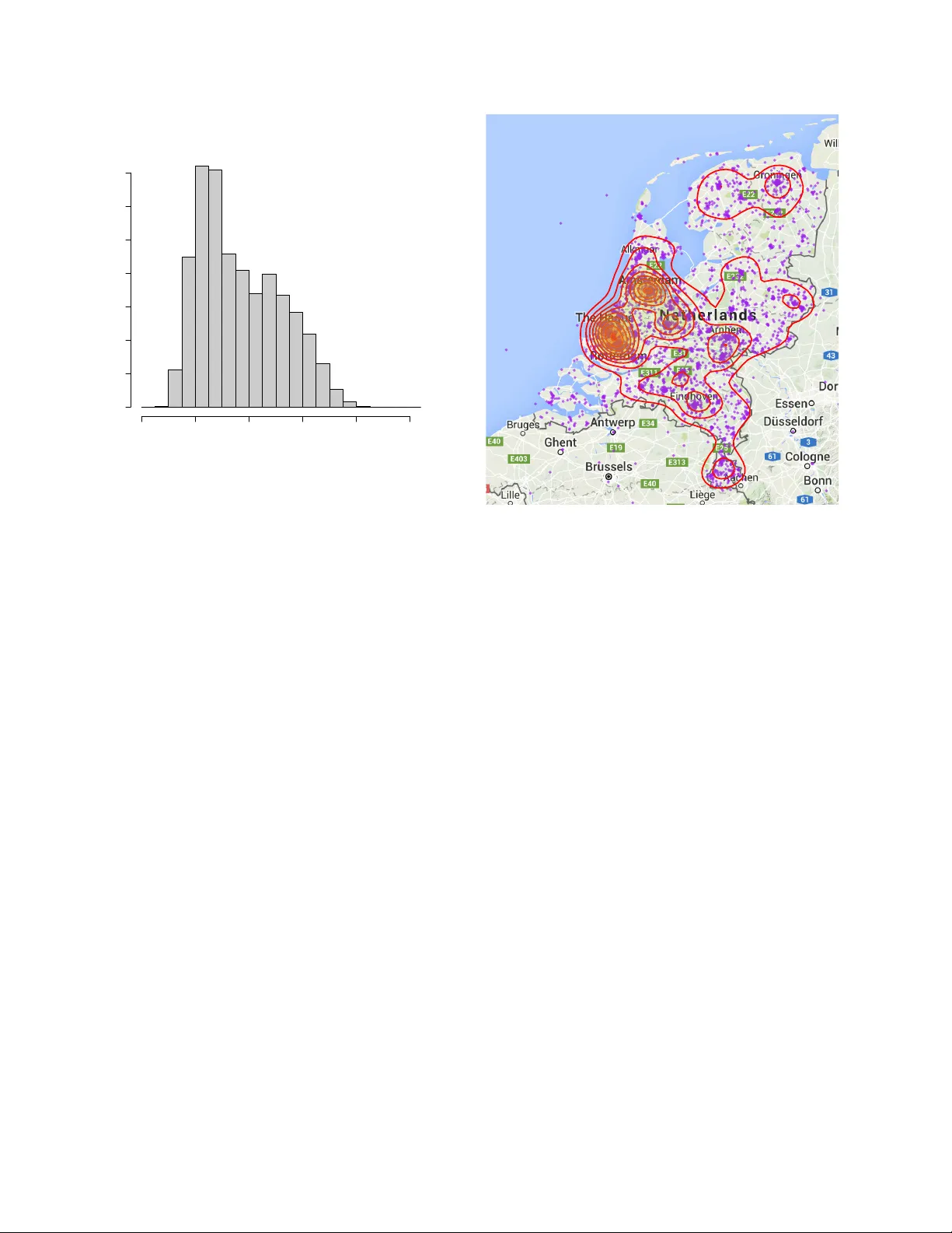
The “Spr ekend Nederland” pr oject and its application to accent location David A. van Leeuwen 1 , 2 , Rosemary Orr 2 1 CLST/CLS, Radboud Uni versity Nijme gen, The Netherlands 2 Nov oLanguage, Nijme gen The Netherlands, 3 Uni versity Colle ge Utrecht, The Netherlands d.vanleeuwen@let.ru.nl , r.orr@uu.nl Abstract This paper describes the data collection effort that is part of the project Spr ek end Nederland ( The Netherlands T alking ), and discusses its potential use in Automatic Ac- cent Location. W e define Automatic Accent Location as the task to describe the accent of a speaker in terms of the location of the speaker and its history . W e discuss possi- ble ways of describing accent location, the consequence these have for the task of automatic accent location, and potential ev aluation metrics. 1. Introduction Automatic accent recognition from speech is tradition- ally treated as a classification task. This matches quite well with our intuitiv e idea of accents, namely , the infor- mation in the speech signal that reveals the membership of a social group, e.g., fellow country members, people of the same social class, or ethnic background. One of the earlier attempts to co ver sev eral accent re- gions in the US for speech research was the collection of the TIMIT database [1]. In this data collection, a to- tal of 439 speak ers were recruited from eight dialect re- gions [2]. This data was used by Hansen et al. [3] for ac- cent classification between se ven of these dialect re gions, where it was concluded that the TIMIT dialects were highly confusable with just two of the dialects, which at- tracted 60 % of all classifications. A more recent study in v olving accent classification is carried out by Behra- van et al. [4], where discrimination between eight foreign accents of Finnish was studied within an i-vector frame- work. Bahari et al. [5] also studied foreign accent classifi- cation, where the multilingual part of the Mixer database recordings from NIST Speaker Recognition Evaluations 2008 and 2010 was used to carry out accent recognition on fiv e foreign accents of English. In a comprehensive study Hanani et al. [6] report on both automatic and hu- man recognition of geographically close accents: 14 ac- cents of the Accents of the British Isles corpus, as well as two accents from different Ethnic groups of the V oices acr oss Birmingham corpus. Accent recognition was introduced in the NIST con- text of speech technology ev aluations in 1996 [7], where the distinction was made between the languages Gen- eral and Southern American English, mainland and T ai- wanese Mandarin, and Caribbean and “highland Span- ish. ” In NIST Language Recognition Ev aluations (LREs), the classification task is cast as a detection task. This is done in order to include a sense of calibration and to fac- tor out the influence of the prior . In 2005 the interest in accent classes was re viv ed, dis- criminating between American and Indian English, and mainland and T aiwanese Mandarin. In 2007 two addi- tional accent pairs were introduced: Caribbean and non- Caribbean Spanish, and Hindi and Urdu. The latter con- trast is often percei ved as cultural or political, with many linguists considering the two languages to be the same. One of the LDC annotators noted that the similarity in recordings of Hindi and Urdu makes it very difficult to distinguish between the two. 1 Recently , in 2015, more focus to dif ferent accents has been gi v en by defining lan- guage clusters [8]. For the clusters Arabic, Chinese, and English, respectively , fiv e, four and three regional accent variants are defined as separate classes to be recognized, as well as a cluster Iberian containing three regional ac- cent variants of Spanish. Since NIST LRE 2007 the lan- guage recognition task is not only e v aluated in terms of detections costs, but also in terms of a logarithmic scoring rule assessing a probabilistic expression of the language classes [9]. Human perception of accents is probably more a clas- sification task than a detection task. From an ev olution- ary perspective, classification of accents might have ad- vantages of quickly discriminating betweens friends and foes, and of assessing potential threats and opportunities in dealing with people from outside the local community . When we hear someone speaking whom we do not know , the first intuiti v e question which arises is: Where is this person fr om? In this question “where” is not limited to geographical location, b ut includes social communities. In human perception, the classes and priors v ary from lis- tener to listener , and will be influenced by the mobility of the listener and exposure to speech from other social groups. 1 As mentioned by George Doddington at the 2007 LRE workshop. In this paper we would like to generalize the accent classification task to one that is closer to the intuitive hu- man perception question “where does this person come from?”. W e will do this along the lines of the informa- tion that is collected in the Dutch project Spr ekend Ned- erland , which might be translated freely as “The Nether- lands T alking. ” Spr ekend Nederland is a project whose goal is to make an in ventory of the accents spoken in the Netherlands, and research the attitudes of people to- wards others with a different accent. Data is collected by means of an application (app) on a smartphone, which implements speech acquisition and playback, and meta- data and attitude entry . The metadata that is important for this paper is information about where people liv ed dur- ing their life, as well as what accent others percei ve them as having. Additionally , speech recordings are accompa- nied by the device location at the time of the recording, which may rev eal information about the mobility of the participants. The data is being collected over a period of a year . T w o months after the start we hav e about 5000 participants. The data is very heterogenous, with v arying amounts of audio and metadata per participant. This is a result of the inclusive design and v oluntary nature of participation. Accent data collection from multiple regions can be problematic, as was shown by Bock and Shamir [10] who used the eight regional accents in the V oxforge crowd- sourcing effort. The authors were able to sho w perfect ac- cent classification by just using a second of silence from each V oxforge recording. Clearly this is not an effect of accent, but of regional difference in recording quality or technical parameters. This paper is organized as follows. First we will de- scribe the efforts and the data characteristics of the Spr ek- end Nederland project, and then formally introduce the task of accent location that can be researched with this kind of data. W e will conclude by discussing potential ev aluation metrics for this task. 2. The Sprek end Nederland project Spr ekend Nederland is a project initiated by the Dutch broadcast organisation NTR, and is partly inspired by the UCU Accents project [11] that studies accent con- ver gence in a community of under graduate students in an international College. Sprekend Nederland , howe ver , has its focus on accent variability and attitude towards spoken accents. The NTR is supported by a group of researchers from v arious disciplines, who see the opportunities that are presented for their own research by this data collec- tion effort. The intention is to make the data available to the research community at the end of the project. 2.1. Data acquisition There are three primary kinds of data collected in the project: audio material (spoken utterances), attitude data (judgements about other participants’ speech) and meta- data (information about the participants themselves). All three forms of data are collected using an app that runs on a smartphone or tablet. The app is dev eloped by a third party for the NTR, as a nativ e application to the iOS and Android platforms. Audio is recorded through the de vice’ s current micro- phone(s), which usually will be the built-in microphone but may also be a head set or remote microphone. One- or two-channel recordings are made at 44.1 kHz and com- pressed using a conservati ve AA C compression at ap- proximately 110 kb/s. This format is some what alien to the speech community , but it was chosen by the app de- veloper to enhance cross-de vice interoperability . Infor- mal listening suggest that the recording quality of current day smartphones and tablets is actually very high. The start of the recording is initiated by the participant, who also controls the end of the recording in most cases. Af- ter a recording, there is an opportunity to play back the recording just made, and if the participants are not satis- fied with the first attempt(s) they can re-record an utter- ance. Metadata and attitude data are acquired by prompt- ing a question, and recording the action in one of four response categories: 1. A discrete slider, with labels at the minimum (left) and maximum (right), with optionally a current value abo ve the slider position. 2. “Y es” or “No” buttons 3. A list of items that each can be selected individu- ally 4. A location on a map, with free pan and zoom For metadata , the question is about the participant, and there are currently 53 metadata questions. For this paper , potentially rele vant questions are: “ Hav e you al- ways li ved at the same location? ”, “ How long ago did you mov e to your current location? ”, “ Where hav e you liv ed the longest within the Netherlands? ”, “ Where do you come from? ”, “ Where did you go to primary school? ”, “ Where did you go to secondary school? ”, “ What is your nativ e language? ”, “ Do you speak a Dutch dialect? ”, “ Where would you locate your accent on a map? ”, as well as demographic questions about sex, age, etc. For attitude data the participant first listens to some- one else recorded earlier . Then, attitude questions like “ W ould you like to have this person as your neighbours? ” follow . For this paper, relev ant questions in this cate- gory of 38 questions are: “ Where does this speak er come from? ”, “ Is this a nati ve speak er of Dutch? ”, “ How far away from you do you think the speaker lives? ”, “ Can you locate the speaker on a map? ” and perhaps “ How old do you think this person is? ”. 2.2. Recruitment of participants Participants are recruited through traditional and social media. Potential participants are encouraged to install the app on their telephone. After installing, the app displays sev eral pages in which the ov erall intention and opera- tion is con veyed. Further use of the app requires reg- istration. The purpose of registration is to ensure that each participant’ s data is associated with that participant only . T o this end, a participant provides an e-mail ad- dress. Howe ver , in the implementation, this e-mail ad- dress is separated from other data in such a way that the researchers working with the data do not ha ve access to this information—ev erything is stored under a numeric participant ID. A third party has access to the email- adresses to handle password resets and requests to be re- mov ed from the database. With registration participants agree to terms and conditions, and approv e the use of data entered in the app for use in the project and for scientific research. For participants under 18, parents or guardians are required to agree to the terms and conditions. T raditional media e vents, such as the mentioning of the app on public radio and television broadcasts, ap- pears to be a dominant factor in the recruitment and ac- tivity of participants. This may be appreciated from Fig- ure 1, which shows the daily rate at which recordings were made after an initial launching which was accom- panied by some exposure on TV and radio. A second boost in recording rate occurred after a documentary on national television about the project at 28 Jan 2016. 2.3. Spoken content and sessions Sev eral kinds of stimulus material are used in order to elicit speech. W e drew our material from six lists of items. These lists were composed by se veral researchers from different research institutes across the Netherlands. List 1 consists of 10 sentences and 44 words, which, to- gether , cover all known regional phonemic variability in the country . List 2 consists of 122 loan words, for which it is most likely that the y display a speaker’ s natural ac- cent. List 3 consists of 100M sentences drawn from the CO W corpus (“COrpus from the W eb”) [12] for max- imum lexical variability , but was toned down to about 2000 sentences for operational reasons. List 4 consists of 66 hand dra wn pictures, used to elicit re gional varying lexical items. List 5 consists of 204 words which cover all possible consonant-vo wel pairs that are used in Dutch. Finally , list 6 consists of nine description tasks used to elicit spontaneous speech. Stimulus material consisting of sentences is presented as a reading task. Material consisting of words is pre- sented as a paced reading task, where at fixed time in- tervals, the next word is sho wn in groups of five words. Dec 01 Dec 15 Jan 01 Jan 15 Feb 01 0.1 0.2 0.5 1.0 2.0 5.0 10.0 Rate of receiving recordings date recordings / minute Figure 1: Rate at which speech recordings are made right after the launch. Data points represent averages o ver cal- endar days, the fitted line represents exponential decay from 2 Dec 2015 (the launch) until 18 Jan 2016. The pictures are shown a short while after which the item must be spoken within a fixed time frame. Each list has its o wn target regarding completeness: for List 1, the goal is that every participant completes all sentences and words. For the other lists, material is ran- domly sampled for each participant. Because of the large number of items to be recorded, all stimulus material is categorized by topic, where there are six possible top- ics. These topics quite naturally get the interpretation of a session , where recordings, attitude questions and meta- data questions are mixed in order . Because it takes a fair amount of time to complete a topic (about 20 min), we expect participants to pace the completion of all topics ov er a longer period of time. In this way , we hope to cov er extended periods of time and different sessions for the same speaker . Where in speaker recognition research, it is impor- tant to hav e recordings of the same speaker through dif- ferent channels and recording devices, such variability is expected to be small in this collection. 3. Some early statistics of participation In this section we will present some early results in the data collection, as inspiration for potential speech tech- nological tasks related to accent recognition that we can use on the data. The data from Figure 1 shows the participation af- ter the initial launch. The exponential fit is made from the launch media ev ent until 18 Jan 2016, where a video Histogram of age participant's age Frequency 0 20 40 60 80 100 0 50 100 150 200 250 300 350 Figure 2: Age distribution of registered participants about the project was posted on social media, and was viewed about 3k times. Assuming an exponential drop at d = 7 . 1 % per day , as shown by the fitted line, we can make a prediction for the total number of record- ings associated with this e vent as N R 0 / (1 − d ) , where R 0 is the initial rate on the first day after the event, and N = 24 × 60 is the number of minutes in a day . T o opti- mize the amount of data acquired, it is important to keep d lo w via an appealing app design and user experience, and effecti ve use of social media. The rate at which participants register and the rate of answers given follows a similar pattern, with decay con- stants of 8.3 % and 6.6 % per day . The age distribution in Figure 2 shows that young adults hav e the highest representation in the data. W e only have the birth year of 31 % of the participants. There are tw o likely reasons for this. Firstly , any of the ques- tions can be skipped if the participant wants, and sec- ondly , all 53 metadata questions are distributed over all six topics, and participants may hav e not reached the question yet, or even stopped using the app. Participants can of course lie about their age, but distribution does not sho w accumulation at e xtreme v alues which might be expected in the case of untruthful answers. Also, to the question “Did you answer all questions truthfully” (ig- noring the philosophical issues of this question for no w) only 0.5 % answered negativ ely . The gender balance is 57/43 % female/male, with only 0.3 % of the participants indicating “other . ” About 50 % of the participants gav e an answer to the question “ Where do yo u come from? ”. The answers are giv en as a location on a map, where the participant is free to use the pan and zoom capabilities of the smart- l e ve l 0.25 0.50 0.75 0.25 0.50 0.75 l e ve l Figure 3: Self-reported answer to the question “ Where do you come from? ”, as data points (purple) and density contours (red). Graph produced using ggmap [13]. phone’ s map interface. These locations are summarized in Figure 3, both as raw data and density contours. As- suming that the density of population is reflected in the density of the participants, this supports the idea that par - ticipants mostly answer honestly . It is striking that hardly any participants appear to be from Belgium, where ov er half the population speaks Dutch. This is probably a re- sult of the cultural divide between the countries, which hav e separate radio and TV channels and newspapers. The project name, of course, does not immediately sug- gest that speakers from Belgium are invited to participate. 4. Accent location Individual accents are largely formed by interaction with one’ s social group. When these groups are primarily dis- tinguished by social class, we might call the accent a soci- olect , and when the groups are formed by cultural back- ground, e.g., an immigrant population from a common origin, we might call this an ethnolect . Although the set- up of the project is general enough that e vidence of both sources of accents can be found, we will be concerned here only with accent as a result of location. W e will now explore a formal definition of the in- formation that was shown in Figure 3, the answer to the question “ Where do you come from? ”, which we will de- fine as the origin location L . For a person who has liv ed her entire life at the same location x (a vector , e.g., lon- gitude/latitude coordinates), we might define the origin location by L 1 : x . (1) Howe ver , this person will hav e interacted with people in the neighbourhood, and her accent will be formed by these interactions. So it might be better to define where she comes from as a probability distrib ution, that peaks around the location she liv es L 2 : p ( x ) . (2) For someone who has mo ved about in her life, we should include the location history in the distribution, as in L 3 : p  x ( t )  . (3) Here t measure time along her life span. At first sight, this may appear to be an ov er-cautious definition of ori- gin location. Howe ver , (3) is just a general definition, and an actual case might be simplified in description. For instance, the dependence on t may be specified as time intervals over periods where someone liv ed in the same place, and the distrib ution component over x may be cho- sen as a Gaussian, or ev en a δ -distribution. In e very day parlance, we can talk of accents along the lines of definition L 3 . For instance, somebody from Germany who has li ved man y years in New Y ork may be recognized as such from her accent. In forensic speaker analysis, an examiner may express traits of a perpetra- tor’ s accent as having traces from different re gional ac- cents, which also indicates a history lik e L 3 . Note that the probability distribution in (3) can be generalized to include social groups or other accent-influencing factors. In order to arriv e at a more point-like specification of the origin location, we might integrate o ver time L 4 : Z t w ( t ) p  x ( t ) = x  dt, (4) where w ( t ) is a weighting function that incorporates the susceptibility to picking up re gional accents at a certain age. Further marginalizing ov er position, we arrive at L 5 : Z t Z x w ( t ) v ( x ) p  x ( t ) = x  x d x dt, (5) where v ( x ) expresses a relative strength that a local ac- cent has on people exposed to that accent. Definition L 5 is point-like, similar to L 1 , but represents some av- eraged location. Such a description may literally “miss the point” if L 4 has multiple modes located far apart. 4.1. Accent location task In the accent location task, we want to know what the origin location L of a speaker is, given one or more spo- ken utterances s . In its most general form, using def- inition L 3 , the task can be expressed as computing the posterior distribution p  x ( t ) | s  . (6) Admittedly , this is quite a phenomenal task. Howe ver , if we generalize accent location to language, then just rec- ognizing the language l from s already narrows the pos- terior down to something lik e the prior π l  x ( t )  , (7) which can be found by studying demographics statistics in the country where the language is spoken. An e xample of what p  x ( anno 2016 )  could look like if the recog- nized language is Dutch is shown in Figure 3. A similar reasoning holds for the accent location task: in effect it is the task of narrowing down the prior, giv en the evidence s . In most cases we would probably like to integrate ov er time, so that the task becomes slightly less daunting and we are effecti vely using an origin location definition like L 4 or L 2 . W e can express the posterior no w as p ( x | s ) = p ( s | x ) π ( x ) π ( s ) , (8) which shows the importance of the prior π ( x ) —the pop- ulation density—again. 4.2. Point estimates and r egression In most recognition tasks we tend not to gi ve an answer in terms of a probability distrib ution, but rather as single value, a class or a scalar or v ector . One way of producing a vector is by inte grating over position x hyp ( s ) = Z x p ( x | s ) x d x , (9) x ref = Z x p ( x ) x d x . (10) Here, we have made point estimates of both the predic- tion (or hypothesis) and the reference distrib ution. In this way , the accent location has turned into a regression problem. Instead of the mean, we could hav e chosen the maximum of the posterior , i.e., the location of the highest mode. The advantage of turning accent location into a re- gression task is that it is easy to choose an ev aluation metric: something based on the distance between x hyp and x ref would make sense. A disadv antage, howe ver , is that for someone who has lived in two distant locations, e.g., the East and W est coast of the US, the mean location (at the center of the US) does not seem to be representa- tiv e of this person’ s origin location. 4.3. Regional aggregates and classification A middle ground between a full spatial distribution and a point estimate is an integration over a geographical re- gion. Examples of such regions are city districts, mu- nicipalities, provinces, and countries. These are cultural- political entities, but for our analysis, any tessellation of Sprekend Nederland participation 1.0 to 3.5 3.5 to 6.5 6.5 to 10.5 10.5 to 15.5 15.5 to 21.5 21.5 to 29.5 29.5 to 44.5 44.5 to 70.5 70.5 to 116.0 116.0 to 186.0 Missing Figure 4: Number of participants per municipality in the Netherlands. The darkest re gions correspond to the cities Amsterdam and Rotterdam, respectiv ely . Graph produced using tmap [14]. the location space will do. If R i is a set of geographical regions cov ering the location space, the hypothesis and reference can be turned into discrete distributions p hyp ( i | s ) = Z x ∈ R i p ( x | s ) d x (11) p ref ( i ) = Z x ∈ R i p ( x ) d x (12) An e xample of the δ -distributions formed by the purple dots in Figure 3 integrated ov er a tessellation formed by the Dutch municipalities is shown in Figure 4. The dis- crete probabilities ha ve been scaled by the total number of participants, so that in fact counts per municipality are shown. This graph shows participants to Sprekend Ned- erland , but of course if one wants to set a region prior π ( i ) it is better to use population statistics. W ith a probability distrib ution ov er regions, it is easy to do accent classification , by simply choosing the re gion with maximum posterior probability: c hyp = arg max i p hyp ( i | s ) , (13) c ref = arg max i p ref ( i ) . (14) This formulation is what is usually used in accent recog- nition research. 5. Evaluation metrics W ith our general task (6) we ha ve not only set a challenge to the engineer, who has to devise methods to produce the required distribution. W ith the corresponding defini- tion of origin location (3), we have also made it hard for an ev aluator to find out how well an accent location sys- tem performs, and for the user , who has to interpret this. In this section we will consider some ev aluation metrics that may be appropriate to the various tasks defined in Section 4. W e want to concentrate on properties of an e valuation metric that are important for de veloping an accent loca- tion system, i.e., a better value should somehow represent a more useful system in general. Properties to consider are 1. Probabilistic interpretation. A probabilistic state- ment about a location should not be an under- or ov erestimation when ev aluated ov er a collection of trials. 2. Sense of distance. A hypothesis location closer to a reference location should be ev aluated as better . Bahari and V an hamme [15] hav e a comprehensive ov erview of ev aluation metrics that consider the or der of classes, e.g., in age groups, as well as the probability of the classes. They also introduce a metric called Nor - malized Ordinal Distance, and show by examples how this has better properties than existing metrics. A com- pletely dif ferent approach is made by Br ¨ ummer and Du Preez [16] who focus on the probabilistic specification of classes and calibration. An important concept in this work is a pr oper scoring rule , a function whose e xpected value is optimum when the predicted probability distri- bution is equal to the actual probability distribution. The NIST primary ev aluation metrics C det and C primary in speaker recognition, as well as C avg in language recogni- tion, are examples of proper scoring rules. These metrics probe the calibration abilities of the predictor in one or a few points in the space of decision cost functions. By contrast, metrics based on logarithmic scoring rules such as C llr [16, 17] integrate o ver the entire space of decision cost functions 2 . A generalization of C llr to more than one class was made in [9] for language recognition, and the deriv ation of the logarithmic scoring rule for multiclass systems can be found in [18]. For predictions of contin- uous probability density functions, a logarithmic scoring rule ne gative log pr edictive density was defined as pri- mary ev aluation metric in the Evaluating Predictive Un- certainty Challenge [19] of the P ASCAL project. In the followup of the challenge, K ohonen and Suomela [20] showed some serious flaws in this metric, and proposed a metric that is sensitiv e to distance, the continuous ranked pr obability scor e . These metrics were studied in assess- ing predicted probability densities in age recognition [21] and were further analyzed in terms of minimum age de- tection. 2 This happens with a particular weighting, which might not corre- spond to the prior interest of the user . 5.1. Local metrics W e start with considering a metric for the case of regional aggregates and classification of Section 4.3. When both reference (12) and hypothesis (11) are a probability dis- tribution over classes, a candidate performance metric is the cross entropy between reference and hypothesis dis- tributions, a veraged ov er the trial set T H region ( ref, hyp ) = − 1 |T | X t ∈T X i p t ref ( i ) log p t hyp ( i ) . (15) This metric is called local because no benefit is gained by having posterior weight in regions neighbouring the regions where the true probability density is. The cross entropy is an error metric (low values are better), is non- negati ve, and only zero if p ref is 1 for e xactly one region, and p hyp as well, for the correct re gion. Howe ver , if p hyp vanishes for classes with finite p ref , the error can be un- bounded. The prior distribution is of influence to the cross en- tropy . A reference value could therefore be formed by inserting the prior π ( i ) in place of p t hyp ( i ) in (15). If the set of trials are drawn from the same prior distrib ution, this reference value reduces to the entropy of the prior . This entropy H ( π ) for the data sho wn in Figure 4 is 5.40, for real population statistics it is 5.48. W e can also aim at removing the influence of the prior . This would lead to something similar to multi- class C llr [9], except that our reference is formed by a distribution over accent regions, rather than being lim- ited to a single region. It is debatable whether the prior should be factored out in accent location, as we are used to in speaker and language recognition. W e might take the stand that knowing where people live is part of the task of figuring out where someone comes from, just lik e knowing the prior o ver word sequences is considered part of the task in speech recognition. 5.2. Distance-sensitive metrics When the accent location task is formulated as a re- gression problem (10), we can easily build in distance- sensitivity in the ev aluation metric. W e can simply define a distance-based error function E regression ( ref, hyp ) = 1 |T | X t ∈T D ( x t ref , x t hyp ) , (16) where D ( x , y ) is some distance function dependent on x and y . The Euclidean distance is a viable candidate, but we can think of more advanced functions as well. For instance, we may want D to be saturated when the Eu- clidian distance becomes too large, or we might want to let D depend on the population density between x and y . For an accent location task of (8) with continuous probability density functions, we would like to assess both probability calibration and distance. W e know that a simple log scoring rule like the negati ve log predictiv e density can be misused [20] and is further not distance- sensitiv e. The continuous ranked probability score [20], and also normalized ordinal distance [15], work by com- paring cumulative distribution functions between refer- ence and hypothesis. For a scalar predictor with natural order , like age, such cumulativ e distribution can be made, but for a two-dimensional predictor , location, it is not im- mediately clear how we can generalize this. One metric that is worth inv estigating, is the integral ov er both probability density functions, weighted by a distance function. For a single trial this would be along the lines of E dist = Z x Z y p ( x | s ) p ( y ) D ( x , y ) d x d y . (17) Such a metric is not ideal. Even if p ( x | s ) = p ( x ) , i.e., the recognizer predicts the accent distribution exactly , the error is not zero, and will depend on the reference p ( x ) . It will take more research to study the properties of (17) and similar distance-aw are metrics for comparing probability distributions. 6. Conclusions In this paper we hav e introduced a new task in speech technology , Accent Location . This is inspired by the de- scriptiv e statistical analysis of the on-going data collec- tion project Spr ekend Nederland , in which already o ver 5000 people are participating. The project may be one of the first of its kind collecting speech, attitude and meta- data on a lar ge scale using modern mobile telephones and utilizing both traditional and social media for recruiting participants. W e believe that this data collection mak es it possible to research accent location as a speech tech- nological task. Accent location in its most fundamental form will be very challenging, depending on what e xactly is required in the task and what the geographical accent variation and distrib ution of speakers is. W e have further explored a number of e valuation metrics that may be suit- able for specific accent location tasks. 7. References [1] Lori F . Lamel, Robert H. Kassel, and Stepanie Sen- eff, “Speech database dev elopment: Design and analysis of the acoustic-phonetic corpus, ” in Speec h Input/Output Assessment and Speech Databases , 1989. [2] V ictor Zue, Stepanie Senef f, and James Glass, “Speech database de velopment at MIT: TIMIT and beyond, ” Speech Communication , v ol. 9, pp. 351– 356, 1990. [3] John H. L. Hanson, Umit H Y apanel, Rongqing Huang, and A yako Ikeno, “Dialect analysis and modeling for automatic classification., ” in INTER- SPEECH , 2004. [4] Hamid Behra van, V ille Hautam ¨ aki, and T omi Kin- nunen, “Factors affecting i-v ector based for- eign accent recognition: A case study in spoken finnish, ” Speech Communication , v ol. 66, pp. 118– 129, 2015. [5] Mohamad Hasan Bahari, Rahim Saeidi, Hugo V an hamme, and David A. van Leeuwen, “ Accent recog- nition using i-vector , gaussian mean supervector and gaussian posterior probability supervector for spontaneous telephone speech, ” in Pr oc. ICASSP , 2013, pp. 7344–7348. [6] Abualsoud Hanani, Martin J Russell, and Michael J Carey , “Human and computer recognition of re- gional accents and ethnic groups from british en- glish speech, ” Computer Speech & Language , v ol. 27, no. 1, pp. 59–74, 2013. [7] “The 1996 NIST language recognition ev aluation plan, ” http://www.itl.nist.gov/iad/ mig/tests/lre/1996/LRE96EvalPlan. pdf , 1996. [8] “The 2015 NIST language recognition ev aluation plan, ” http://www.nist.gov/itl/iad/ mig/upload/LRE15_EvalPlan_v23.pdf , 2015. [9] Niko Br ¨ ummer and David A. van Leeuwen, “On calibration of language recognition scores, ” in Pr oc. Odysse y 2006 Speaker and Language recognition workshop , San Juan, June 2006. [10] Benjamin Bock and Lior Shamir , “ Assessing the ef- ficacy of benchmarks for automatic speech accent recognition, ” in Pr oceedings of the 8th Interna- tional Conference on Mobile Multimedia Commu- nications . ICST (Institute for Computer Sciences, Social-Informatics and T elecommunications Engi- neering), 2015, pp. 133–136. [11] Rosemary Orr, Hugo Quen ´ e, Roeland van Beek, Thari Diefenbach, Da vid A. van Leeuwen, and Mar- ijn Huijbregts, “ An international English speech corpus for longitudinal study of accent dev elop- ment, ” in Proc. Inter speech . ISCA, August 2011. [12] Roland Sch ¨ afer , “Processing and querying large web corpora with the co w14 architecture, ” in Pr o- ceedings of the 3r d W orkshop on Challenges in the Mana gement of Lar ge Corpor a (CMLC-3) , Pi- otr Ba ´ nski, Hanno Biber, Ev elyn Breiteneder , Marc Kupietz, Harald L ¨ ungen, and Andreas Witt, Eds., 2015, pp. 28–34. [13] David Kahle and Hadley W ickham, “ggmap: Spa- tial visualization with ggplot2, ” The R Journal , vol. 5, no. 1, pp. 144–161, 2013. [14] Martijn T ennekes, tmap: Thematic Maps , 2015, R package version 1.2. [15] Mohamad Hasan Bahari and Hugo V an hamme, “Normalized ordinal distance; a performance metric for ordinal, probabilistic-ordinal or partial-ordinal classification problems, ” in Case Studies in Intel- ligent Computing: Achievements and T rends , Nau- man Israr Biju Issac, Ed., pp. 285–302. CRC Press, T aylor and Francis, 2014. [16] Niko Br ¨ ummer and Johan du Preez, “ Application- independent ev aluation of speaker detection, ” Com- puter Speech and Language , vol. 20, pp. 230–275, 2006. [17] David A. van Leeuwen and Niko Br ¨ ummer , “ An in- troduction to application-independent ev aluation of speaker recognition systems, ” in Speak er Classifi- cation , Christian M ¨ uller , Ed., v ol. 4343 of Lectur e Notes in Computer Science / Artificial Intelligence . Springer , 2007. [18] Niko Br ¨ ummer , Measuring, r efining and calibr at- ing speaker and language information extracted fr om speech , Ph.D. thesis, Stellenbosch University , 2010. [19] Joaquin Qui ˜ nonero-Candela, Carl Edward Ras- mussen, Fabian Sinz, Olivier Bousquet, and Bern- hard Sch ¨ olkopf, “Evaluating predictiv e uncertainty challenge, ” vol. 3944 of Lectur e Notes in Com- puter Science , pp. 1–27. Springer Berlin / Heidel- berg, 2006. [20] Jukka Kohonen and Jukka Suomela, “Lessons learned in the challenge: Making predictions and scoring them, ” vol. 3944 of Lectur e Notes in Com- puter Science , pp. 95–116. Springer Berlin / Heidel- berg, 2006. [21] David A. van Leeuwen and Mohamad Hasan Ba- hari, “Calibration of probabilistic age recognition, ” in Pr oc. Interspeech , Portland, 2012, ISCA.