Kernel Methods for the Approximation of Nonlinear Systems

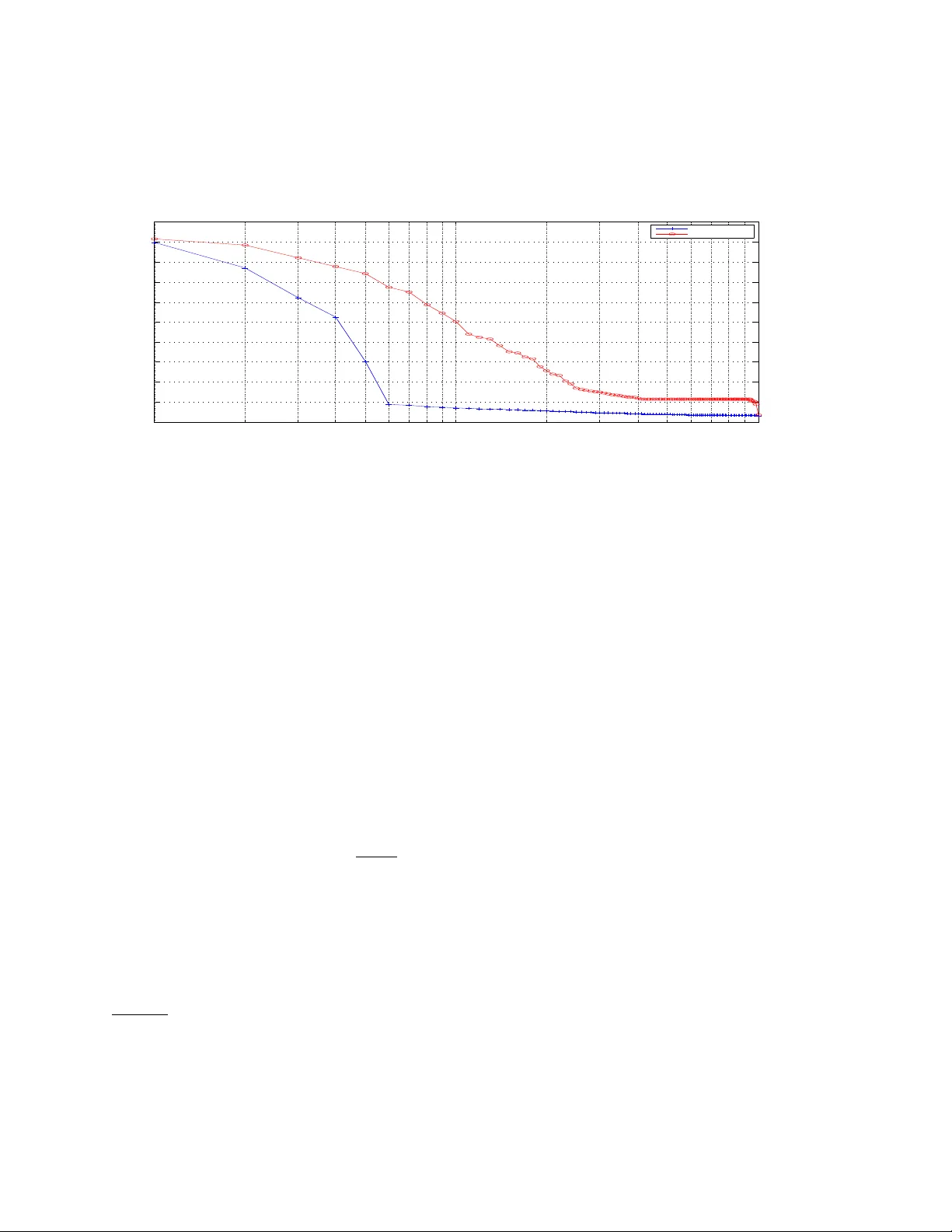
KERNEL METHODS F OR THE APPR O XIMA TION OF NONLINEAR SYSTEMS JAKE BOUVRIE † ¶ AND BOUMEDIENE HAMZI ‡ ¶ Abstract. W e introduce a data-driven model approximation method for nonlinear control systems, dra wing on recent progress in mac hine learning and statistical dimensionality reduction. The method is based on em b edding the nonlinear system in a high (or inﬁnite) dimensional repro ducing kernel Hilb ert space (RKHS) where linear balanced truncation ma y b e carried out implicitly . This leads to a nonlinear reduction map which can b e combined with a represen tation of the system belonging to a RKHS to giv e a closed, reduced order dynamical system which captures the essential input-output c haracteristics of the original model. W orking in RKHS provides a conv enient, general functional-analytical framework for theoretical understanding. Empirical simulations illustrating the approach are also provided. 1. In tro duction. Data-based mo delling of nonlinear dynamical systems has b een addressed b y many authors. F or example, several methods hav e been dev el- op ed in Time Series Analysis ([19] for example) and System Iden tiﬁcation ([52], [51] for example). Coifman et al. discuss data-based mo delling of a sto c hastic Langevin system [9]. Archam b eau et al. [2] prop osed metho ds to appro ximate SDEs from data. Smale and Zhou use k ernel metho ds to approximate a hyperb olic dynamical system [45]. In this pap er we prop ose a sc heme for the approximation of nonlinear systems using balanced mo del-order reduction. A key , and to our knowledge, no vel p oint of departure from the literature on nonlinear mo del reduction is that our approac h marries appro ximation and dimensionality reduction metho ds kno wn to the machine learning and statistics comm unities with existing ideas in linear and nonlinear con- trol. In particular, w e apply a method similar to kernel PCA (Principal Comp onent Analysis) as well as function appro ximation in Reproducing Kernel Hilbert Spaces (RKHSes) to the problem of balanced mo del reduction. W orking in RKHSes provides a con venien t, general functional-analytical framew ork for theoretical understanding as w ell as a ready source of existing results and error estimates. The approach presen ted here is also strongly empirical, in that observ abilit y and controllabilit y , and in some cases the dynamics of the nonlinear system are estimated from simulated or measured tra j ectories. The approach we prop ose begins b y viewing the con trollability and observ abilit y energies for nonlinear systems as Gramians in a high (or p ossibly inﬁnite) dimen- sional RKHS. These Gramians are appro ximated empirically and then simultaneously diagonalized in order to iden tify directions which, in the RKHS, are b oth the most observ able and the most controllable. The assumption that it is p ossible to apply the metho d of linear balancing to a nonlinear system when lifted to a RKHS is far more reasonable than applying the linear theory in the original space hoping for the b est. W orking in the high dimensional RKHS allows one to p erform linear op erations on a representation of the system’s state and output which can capture strong nonlinearities. Moreov er, † Laboratory for Computational and Statistical Learning, Massach usetts Institute of T echnology , Cambridge, MA 02138, USA. (jvb@csail.mit.edu) ‡ Department of Mathematics, Imperial College London, London SW7 2AZ, UK. (b.hamzi@imperial.ac.uk) ¶ Parts of this w ork were done while b oth authors were at Departmen t of Mathematics, Duke Universit y , Durham, NC 27708, USA. 1 w orking in an RKHS readily include linear spaces 1 and, therefore, our approach not only cov ers existing Linear Theory but also extends the range of av ailable spaces where it is reasonable to assume that one will obtain b etter results when dealing with a nonlinear problem. Therefore, a system for which existing mo del reduction methods fail, may b e appro ximated by a low er dimensional system when mapp ed in to a RKHS. This situation closely parallels the problem of linear separabilit y in data classiﬁcation: A dataset whic h is not linearly separable migh t b e easily separated when mapped into a nonlinear feature space. The decision b oundary is linear in this feature space, but is nonlinear in the original data space. Essen tially , we are proposing to apply linear metho ds to nonlinear systems once mapped in to a high (p ossibly inﬁnite-dimensional) Hilb ert space 2 . Nonlinear reduction of the state space already allows to the design of simpler con trollers, but is only half of the picture. One w ould also like to be able to write a closed, reduced dynamical system whose input-output behavior closely captures that of the original system. This problem is the focus of the second half of our pap er, where w e again exploit helpful properties of RKHS in order to pro vide such a closed system. The paper is organized as follows. In the next section w e pro vide the relev an t bac kground for mo del reduction and balancing for linear and nonlinear control sys- tems. W e then adapt and extend balancing techniques describ ed in the background section to the current RKHS setting in Section 3. Section 4 then prop oses a method for determining a closed, reduced nonlinear control system in light of the reduction map describ ed in Section 3. Finally , Section 5 provides exp erimen ts illustrating an application of the prop osed methods to some nonlinear systems where the metho d of linear balancing do es not apply in R n since the systems we simulated are not linearly con trollable and the origin is not asymptotically stable but the same metho d of linear balancing applies to the nonlinear system after being lifter to a RKHS. App endix A con tains a review of Learning Theory , App endix B contains a description of k ernel PCA. Preliminary results of this work can b e found in [5, 6]. 2. Bac kground. Several approaches hav e b een prop osed for the reduction of lin- ear con trol systems in view of con trol, but few exist for ﬁnite or inﬁnite-dimensional nonlinear con trol systems. F or linear systems, the pioneering “Input- Output balanc- ing” approac h prop osed b y B.C. Mo ore [29] observes that the important states are the ones that are both easy to reac h and that generate a lot of energy at the output. If a large amoun t of energy is required to reac h a certain state but the same state yields a small output energy , the state is unimp ortant for the input-output behavior of the system. The goal is then to ﬁnd the states that are b oth the most controllable and the most observ able. One w ay to determine suc h states is to ﬁnd a change of coordinates where the controllabilit y and observ abilit y Gramians (which can be viewed as a mea- sure of the controllabilit y and the observ ability of the system) are equal and diagonal. States that are diﬃcult to reac h and that don’t signiﬁcan tly aﬀect the output are then ignored or truncated. A system expressed in the co ordinates where each state is 1 When using the embedding Φ : x 7→ x and kernel k ( x, y ) = h x, y i , cf. Appendix A for meaning of these ob jects. 2 Let us note here that it is important to c ho ose the right RKHS in order to p erform this sort of computations. In our work, we used existing Universal Kernels such as the Gaussian or polynomial kernels (cf. Prop osition A.4) but, in general, properly choosing the right RKHS is an op en problem even in classical Learning Theory . 2 equally con trollable and observ able is called its b alanc e d r e alization . A prop osal for generalizing this approac h to nonlinear con trol systems w as ad- v anced b y J. Scherpen [36], where suitably deﬁned con trollabilit y and observ abil- it y energy functions reduce to Gramians in the linear case. In general, to ﬁnd the balanced realization of a system one needs to solv e a set of Hamilton-Jacobi and Ly apunov equations (as we will discuss b elow). Mo ore [29] prop osed an alternative, data-based approac h for balancing in the linear case. This metho d uses samples of the impulse resp onse of a linear system to construct empirical controllabilit y and observ- abilit y Gramians which are then balanced and truncated using Principal Comp onents Analysis (PCA, or Prop er Orthogonal Decomp osition (POD) [17]). This data-driv en strategy was then extended to nonlinear con trol systems with a stable linear appro x- imation b y Lall et al. [25], by eﬀectively applying Moore’s metho d to a nonlinear system by wa y of the Galerkin pro jection. Despite the fact that the balancing theory underpinning their approach assumes a linear system, Lall and colleagues were able to eﬀectiv ely reduce some nonlinear systems. Phillips et al. [32] has also studied reduction of nonlinear circuit mo dels in the case of linear but un balanced coordinate transformations and found that approximation using a polynomial RKHS could oﬀer computational adv antages. Gra y and V erri- est mention in [15] that studying algebraically deﬁned Gramian op erators in RKHS ma y pro vide adv an tageous appro ximation properties, though the idea is not further explored. Finally , Coifman et al. [9] discuss reduction of an uncontrolled sto c has- tic Langevin system. There, eigenfunctions of a combinatorial Laplacian, built from samples of tra jectories, provide a set of reduction coordinates but does not provide a reduced system. This method is related to k ernel principal comp onents (KPCA) using a Gaussian kernel, ho wev er reduction in this study is carried out on a simpliﬁed linear system outside the context of con trol. In the following sections we review balancing of linear and nonlinear systems as in tro duced in [29] and [36]. See also [37] for a go o d surv ey on balancing for linear and nonlinear systems. 2.1. Balancing of Linear Systems. Consider a linear con trol system ˙ x = Ax + B u, y = C x, , (2.1) where ( A, B ) is con trollable, ( A, C ) is observ able and A is Hurwitz. W e deﬁne the con trollability and the observ ability Gramians as, respectively , W c = R ∞ 0 e At B B > e A > t dt, and W o = R ∞ 0 e A > t C > C e At dt. These tw o matrices can b e viewed as a measure of the con trollability and the observ- abilit y of the system [29]. F or instance, consider the past energy [36, 35], L c ( x 0 ), deﬁned as the minimal energy required to reach x 0 from 0 in inﬁnite time L c ( x 0 ) = inf u ∈ L 2 ( −∞ , 0) , x ( −∞ )=0 ,x (0)= x 0 1 2 Z 0 −∞ || u ( t ) || 2 dt, (2.2) and the future energy [36, 35], L o ( x 0 ), deﬁned as the output energy generated by releasing the system from its initial state x ( t 0 ) = x 0 , and zero input u ( t ) = 0 for t ≥ 0, i.e. L o ( x 0 ) = 1 2 Z ∞ 0 || y ( t ) || 2 dt, (2.3) 3 for x ( t 0 ) = x 0 and u ( t ) = 0 , t ≥ 0. In the linear case, it can b e shown that L c ( x 0 ) = 1 2 x > 0 W − 1 c x 0 , and L o ( x 0 ) = 1 2 x > 0 W o x 0 . (2.4) The columns of W c span the con trollable subspace while the n ullspace of W o coincides with the unobserv able subspace. As such, W c and W o (or their estimates) are the key ingredien ts in many mo del reduction techniques. It is also well kno wn that W c and W o satisfy the Lyapuno v equations [29] AW c + W c A > = − B B > , A > W o + W o A = − C > C. (2.5) Sev eral metho ds ha ve b een developed to solve these equations (see [16, 26, 27] for example). As men tioned at the beginning of this section, it is also p ossible to estimate the Gramians from empirical data, cf. (3.4) and (3.6) b elow. The idea behind balancing is to ﬁnd a representation where the system’s observ- able and con trollable subspaces are aligned so that reduction, if p ossible, consists of eliminating the states that are least controllable and which are also the least ob- serv able. More formally , we w ould like to ﬁnd a new co ordinate system such that Σ := W c = W o = diag { σ 1 , · · · , σ n } where σ 1 ≥ σ 2 ≥ · · · ≥ σ n > 0. Theorem 2.1. [11] If ( A, B ) is c ontr ol lable and ( A, C ) is observable, then the eigenvalues of W o W c ar e similarity invariants, i.e. they ar e indep endent of the choic e of the state-sp ac e r epr esentation of (2.1). Mor e over, ther e exists a state-sp ac e r epr e- sentation wher e Σ := W c = W o = diag { σ 1 , · · · , σ n } (2.6) with σ 1 ≥ σ 2 ≥ · · · ≥ σ n > 0 ar e the squar e r o ots of the eigenvalues of W o W c . Such r epr esentations ar e c al le d b alanc e d, and the system is in b alanc e d form. The σ i ’s, i = 1 , ..., n ar e c al le d the Hankel singular values. The state sp ac e expr esse d in the tr ans- forme d c o or dinates ( QAQ − 1 , QB , C Q − 1 ) is b alanc e d and QW c Q > = Q −> W o Q − 1 = Σ wher e Q ∈ R n × n . The Hankel singular v alues, σ i | n i =1 , are the square ro ots of the eigen v alues of W o W c and are the singular v alues of the Hankel op erator H = Ψ o ◦ Ψ c (2.7) that characterizes the input-output b ehaviour of the system (2.1) with Ψ c , the con- trollabilit y op erator, which maps u ∈ L 2 ( −∞ , 0] to x (0) and Ψ o , the observ ability op erator, which maps x (0) to y ( t ), t ≥ 0 with no input applied for t ≥ 0 [11]. More precisely , Ψ c : L 2 ( −∞ , 0] → C n u 7→ R 0 −∞ e − Aτ B u ( τ ) dτ (2.8) and Ψ o : C n → L 2 [0 , ∞ ) x (0) = x 0 7→  C e At x 0 , for t ≥ 0 , 0 , otherwise . (2.9) Clearly , x 0 = Ψ c u ( t ) for u ( t ) ∈ L 2 ( −∞ , 0] is the system state at t = 0 due to the past input and y ( t ) = Ψ 0 x 0 , t ≥ 0 is the future output due to the initial state 4 x 0 with the input set to zero. In fact, H c haracterizes the system’s future output y ( t ) = H u ( t ) , t ≥ 0 based on the past input u ( t ) , t ≤ 0. More precisely , if x ( −∞ ) = 0, H u ( t ) = Ψ o Ψ c u ( t ) = Z 0 −∞ C e A ( t − τ ) B u ( τ ) dτ , for t ≥ 0 (2.10) When H is kno wn to b e a compact operator, then its adjoint op erator H ∗ is also compact and the comp osition H ∗ H is a self-adjoint compact op erator with the spectral decomp osition H ∗ H = ∞ X i =1 σ 2 i h· , Ψ i i L 2 Ψ i , σ i ≥ 0 , (2.11) h Ψ i , Ψ j i L 2 = δ ij , h Ψ i , ( H ∗ H )(Ψ i ) i L 2 = σ 2 i (2.12) where σ 2 i is an eigen v alue of H ∗ H with the corresponding eigenv ector Ψ i , ordered as σ 1 ≥ · · · ≥ σ n > 0 and σ i ≥ n +1 = 0 are the Hankel singular v alues of the input-output system Σ. F or square linear systems, the nonzero eigenv alues of the Hankel op erator asso ciated to the system are the nonzero eigen v alues of the cross Gramian deﬁned as the solution, W x , of AW x + W x A + B C = 0 [37]. W e also hav e, for ev ery x 0 ∈ C n , Ψ c Ψ ∗ c x 0 = W c x 0 , Ψ ∗ o Ψ o x 0 = W o x 0 . (2.13) Th us W c and W o are the matrix represen tations of the op erators Ψ c Ψ ∗ c and Ψ ∗ o Ψ o [11]. F or model reduction, typically one lo oks for a gap in the singular v alues { σ i } for guidance as to where truncation should o ccur. If there is a k suc h that σ k  σ k +1 , then the states most resp onsible for go v erning the input-output relationship of the system are ( x 1 , · · · , x k ) while ( x k +1 , . . . , x n ) are assumed to mak e negligible con tributions. Theorem 2.2. [11] Consider a line ar system (2.1) with its asso ciate d Hankel op er ator H (2.7). L et H k b e the Hankel op er ator of the r e duc e d or der line ar system of or der k . Then, || H − H k || = σ k +1 (2.14) If x (0) = 0 , the err or b etwe en y , the output of the ful l or der system, and y r , the output of the r e duc e d or der system with k state variables, satisﬁes || y − y r || 2 ≤ 2  n X j = k +1 σ j  || u || 2 (2.15) If F is unstable then the controllabilit y and observ ability quantities deﬁned in (2.2) are undeﬁned since the integrals will b e unbounded. There may , ho w ever, still exist solutions to the Ly apunov equations (2.5) when F is unstable [48, 20]. Other ap- proac hes to balancing unstable linear systems exist (see [49, 50, 18, 54] for the metho d of LQG balancing for example). Although several metho ds also exist for computing Q [26, 27], it is common to simply compute the Cholesky decomp osition of W o so that W o = Z Z > , and form the SVD U Σ 2 U > of Z > W c Z . Then Q is giv en b y Q = Σ 1 2 U > Z − 1 . W e also note that the problem of ﬁnding the coordinate c hange Q can be seen as an optimization problem [1] of the form min Q trace[ QW c Q ∗ + Q −∗ W o Q − 1 ]. 5 2.2. Balancing of Nonlinear Systems. In the nonlinear case, the energy func- tions L c and L o in (2.2) and (2.3) are obtained by solving both a Lyapuno v and a Hamilton-Jacobi equation. Here we follow the dev elopment of Sc herp en [36, 37]. Con- sider the nonlinear system Σ :  ˙ x = f ( x ) + P m i =1 g i ( x ) u i , y = h ( x ) , (2.16) with x ∈ R n , u ∈ R m , y ∈ R p , f (0) = 0, g i (0) = 0 for 1 ≤ i ≤ m , and h (0) = 0. Moreo ver, assume the following Hyp othesis. Assumption A: The linearization of (2.16) around the origin is con trollable, observ able and A = ∂ f ∂ x | x =0 is asymptotically stable. The controllabilit y op erator Ψ c : U → X with X = R n and U = L m 2 [0 , ∞ ), and the observ abilit y op erator Ψ o : X → Y with Y = L p 2 [0 , ∞ ) for this system are deﬁned b y Ψ c : u 7→ x 0 :  ˙ x = − f ( x ) − g ( x ) u, x ( ∞ ) = 0 , x 0 = x (0) (2.17) Ψ o : x 0 7→ y :  ˙ x = f ( x ) , x 0 = x (0) , y = h ( x ) (2.18) As in the linear case, Ψ c and Ψ o represen t the input-to-state b ehavior and the state- to-output behavior, respectively . The Hank el op erator for the nonlinear system Σ in (2.16) is given by the composition of Ψ c and Ψ o H := Ψ o ◦ Ψ c (2.19) Consider the norm-minimizing in verse Ψ † c : X → U Ψ † c : x 0 7→ u := argmin Ψ c ( u )= x 0 || u || . (2.20) F rom this p oint of view L c in (2.2) and L o in (2.3) are L c ( x 0 ) := 1 2 || Ψ † c ( x 0 ) || 2 , L o ( x 0 ) := 1 2 || Ψ o ( x 0 ) || 2 (2.21) Theorem 2.3. [36, 35] Consider the nonline ar system Σ deﬁne d in (2.16). If the origin is an asymptotic al ly stable e quilibrium of f ( x ) on a neighb orho o d W of the origin, then for al l x ∈ W , L o ( x ) is the unique smo oth solution of ∂ L o ∂ x ( x ) f ( x ) + 1 2 h > ( x ) h ( x ) = 0 , L o (0) = 0 (2.22) under the assumption that (2.22) has a smo oth solution on W . F urthermor e for al l x ∈ W , L c ( x ) is the unique smo oth solution of ∂ L c ∂ x ( x ) f ( x ) + 1 2 ∂ L c ∂ x ( x ) g ( x ) g > ( x ) ∂ > L c ∂ x ( x ) = 0 , L c (0) = 0 (2.23) under the assumption that (2.23) has a smo oth solution ¯ L c on W and that the origin is an asymptotic al ly stable e quilibrium of − ( f ( x ) + g ( x ) g > ( x ) ∂ ¯ L c ∂ x ( x )) on W . 6 With the controllabilit y and the observ ability functions on hand, the input- normal/output-diagonal realization of system (2.16) can b e computed b y wa y of a co ordinate transformation. More precisely , Theorem 2.4. [36, 35] Consider system (2.16) under Assumption A and the assumptions in The or em 2.3. Then, ther e exists a neighb orho o d W of the origin and c o or dinate tr ansformation x = ϕ ( z ) on W c onverting the ener gy functions into the form L c ( ϕ ( z )) = 1 2 z > z and L o ( ϕ ( z )) = 1 2 P n i =1 z 2 i σ i ( z i ) 2 , wher e σ 1 ( x ) ≥ σ 2 ( x ) ≥ · · · ≥ σ n ( x ) . The functions σ i ( · ) ar e c al le d Hankel singular v alue functions . Analogous to the linear case, the system’s states can b e sorted in order of imp or- tance b y sorting the singular v alue functions, and reduction pro ceeds by remo ving the least important states. In the abov e framework for balancing of nonlinear systems, one needs to solv e (or numerically ev aluate) the PDEs (2.22), (2.23) and compute the co ordinate change x = ϕ ( z ), ho wev er there are no systematic metho ds or tools for solving these prob- lems. V arious approximate solutions based on T a ylor series expansions hav e b een prop osed [23, 22, 13]. Newman and Krishnaprasad [30] introduce a statistical approx- imation based on exciting the system with white Gaussian noise and then computing the balancing transformation using an algorithm from diﬀerential top ology . As men- tioned earlier, an essentially linear empirical approach w as prop osed in [25]. In this pap er, we combine asp ects of both data-driven approaches and analytic approaches b y carrying out linear balancing of nonlinear control systems in a suitable RKHS. 3. Empirical Balancing of Nonlinear Systems in RKHS. W e consider a general nonlinear system of the form  ˙ x = f ( x, u ) y = h ( x ) (3.1) with x ∈ R n , u ∈ R m , y ∈ R p , f (0 , 0) = 0, and h (0) = 0. Let R ( x 0 ) = { x 0 ∈ R n : ∃ u ∈ L ∞ ( R , R m ) and ∃ T ∈ [0 , ∞ ) such that x (0) = x 0 and x ( T ) = x 0 } be the reac hable set from the initial condition x (0) = x 0 . Hyp othesis H: 3 The system (3.1) is zero-state observ able, its linearization around the origin is con trollable, and the origin of ˙ x = f ( x, 0) is asymptotically stable. W e treat the problem of estimating the observ ability and con trollability Gramians as one of estimating an in tegral op erator from data in a repro ducing k ernel Hilb ert space (RKHS) [3], cf. App endix for deﬁnition and k ey results on RKHSes. Our appr o ach hinges on the key mo deling assumption that the nonline ar dynamic al system c an b e emb e dde d in an appr opriate high (or p ossibly inﬁnite) dimensional RKHS wher e the metho d of line ar b alancing c an b e applie d . More precisely , we will essen tially assume that there is an RKHS H and maps Φ , Ψ : R n → H ; x 7→ H such that con trollability and observ ability energies of the nonlinear system (3.1) are “linearized”, i.e. that in H they hav e an expression similar to the one in the linear case (2.4) and, therefore, can b e written as L c ( x ) u 1 2 Φ T ( x ) W − 1 c Φ( x ) , L o ( x ) u 1 2 Ψ T ( x ) W o Ψ( x ) , (3.2) with W c , W o ∈ R N × N , N  n , are very large dimensional matrices 4 . 3 Let us note here that this assumption is similar to Assumption A above and that we made it mainly out of conv enience but is not necessary as illustrated in the 2D and 7D examples b elow. 4 If the system is aﬃne in the input, we will use the PDEs (2.22) and (2.23) to ﬁnd Φ, Ψ, W c and W o . W e leav e such analysis for future work. 7 By “linearization” here, we mean mapping the nonline ar system in a higher di- mensional Hilb ert sp ac e wher e line ar the ory c an b e applie d . T o illustrate this p oin t [46], consider a p olynomial in R , p ( x ) = α + β x + γ x 2 where α , β , and γ are re- als. If we consider the map Φ : R → R 3 deﬁned as Φ( x ) = [1 x x 2 ] T then p ( x ) = α · [1 x x 2 ] T = α · Φ( x ) is an aﬃne polynomial in the v ariable Φ( x ). Another example to illustrate our though t pro cess is the one of Supp ort V ector Mac hines (SVMs) that we referred to in the introduction. More precisely , consider the problem of classifying points in a data set D = (( x 1 , y 1 ) , · · · , ( x n , y n )) with x i ∈ X with X a set and y i = ± 1, i.e. trying to ﬁnd w ∈ R d with || w || 2 = 1 and b ∈ R such that h w, x i i + b > 0 for all i with y i = +1, and h w, x i i + b < 0 for all i with y i = − 1, i.e. that the linear h yp erplane characterized b y ( w , b ) p erfectly separates the set D in to t wo groups of data p oints, the ones with y i = +1 and the ones with y i = − 1. Sometimes, it is p ossible to ﬁnd such an h yp erplane but, in general, ﬁnding a linear h yp erplane that perfectly separates a giv en data set D is not alw ays p ossible and ﬁnding ( w, b ) will not be possible. T o solv e the classiﬁcation problem, the SVM algorithm maps the input data ( x 1 , · · · , x n ) into a (p ossibly inﬁnite-dimensional) Hilb ert space H , the so-called fe atur e sp ac e , by a t ypically nonlinear map Φ : X → H called the fe atur e map . Then one lo oks for a linear hyperplane that separates the data ((Φ( x 1 ) , y 1 ) , · · · , (Φ( x n ) , y n )), i.e. one looks for ( w , b ) in H . When this is possible, the data in D will b e classiﬁed in t wo categories, the ones with y i = +1 and the ones with y i = − 1, but the separating curve for D will not b e a linear hyperplane in the original space (ev en if it is a linear h yp erplane in H ). An imp ortan t property of SVMs is that for every dataset D without contradicting p oints, i.e. ( x i , y i ) and ( x j , y j ) with x i = x j and y i 6 = y j , there exists a feature map that allows the perfect separation b y a h yp erplane in the feature space [47]. Our aim is to generalize this wa y of thinking to nonlinear dynamical systems, i.e. giv en a problem for a nonlinear dynamical system, we map the state v ariables b y a t ypically nonlinear map Φ : X → H where H is (p ossibly inﬁnite-dimensional) Hilbert space in which the computations b ecome simpler 5 . In our case, “simpler” means applying Linear Theory . In this pap er, we will focus on the problem of approximation of nonlinear control systems by applying the method of linear balancing in RKHSes. W e lea ve other applications for future w ork. Co v ariance op erators in RKHSes and their empirical estimates are the ob jects of primary imp ortance and contain the information needed to p erform mo del reduction. In particular, the (linear) observ ability and controllabilit y Gramians are estimated and diagonalized in the RKHS, but capture nonlinearities in the original state space. The reduction approach we prop ose adapts ideas from k ernel PCA (KPCA) [41] and is driv en b y a set of sim ulated or sampled system tra jectories, extending and generalizing the w ork of Mo ore [29] and Lall et al. [25]. Our metho d works quite well since the con trollability and the observ ability en- ergies in the linear case can b e expressed as inner pro ducts (2.4) and working in RKHSes al lows to ﬁnd nonline ar versions of line ar algorithms that c an b e expr esse d in terms of inner pr o ducts (this is the so-called kernel trick in Learning Theory , see App endix A for more explanations). Hence the empirical Gramians deﬁned b elow for nonlinear systems can b e viewed as reasonable approximations of the controllabilit y and observ ability energies for nonlinear systems. In the dev elopment below we lift state vectors of the system (3.1) into a Hilb ert 5 One could also think of the metho ds in Quantum Mechanics where one constructs a Hilbert space from measurements in order to p erform computations. 8 space H , i.e. we consider a mapping Φ : R n → H and analyze the nonlinear system whose state is Φ( x ). 3.1. Empirical Gramians in RKHS. F ollo wing [29], w e estimate the con- trollabilit y Gramian by exciting each coordinate of the input with impulses 6 while setting x 0 = 0. One can also further excite using rotations of impulses as suggested in [25], ho w ever for simplicit y we consider only the original signals prop osed in [29]. Let u i ( t ) = δ ( t ) e i b e the i -th excitation signal, and let x i ( t ) be the corresp onding resp onse of the system. F orm the matrix X ( t ) =  x 1 ( t ) · · · x m ( t )  ∈ R n × m , (3.3) so that X ( t ) is seen as a data matrix with column observ ations giv en b y the respective resp onses x i ( t ). Then W c ∈ R n × n is giv en b y W c = 1 m Z ∞ 0 X ( t ) X ( t ) > dt. (3.4) W e can appro ximate this integral by sampling the matrix function X ( t ) within a ﬁnite time interv al [0 , T ] assuming the regular partition { t i } N i =1 , t i = ( T / N ) i . This leads to the empirical controllabilit y Gramian c W c = T mN N X i =1 X ( t i ) X ( t i ) > . (3.5) As describ ed in [29], the observ ability Gramian is estimated by ﬁxing u ( t ) = 0, setting x 0 = e i for i = 1 , . . . , n , and measuring the corresp onding system output re- sp onses y i ( t ). As b efore, assemble the resp onses into a matrix Y ( t ) = [ y 1 ( t ) · · · y n ( t )] ∈ R p × n . The observ ability Gramian W o ∈ R n × n and its empirical counterpart c W o are giv en b y W o = 1 p Z ∞ 0 Y ( t ) > Y ( t ) dt (3.6) and c W o = T pN N X i =1 e Y ( t i ) e Y ( t i ) > (3.7) where e Y ( t ) = Y ( t ) > . The matrix e Y ( t i ) ∈ R n × p can b e thought of as a data matrix with column observ ations d j ( t i ) =  y 1 j ( t i ) , . . . , y n j ( t i )  > ∈ R n , j = 1 , . . . , p, i = 1 , . . . , N (3.8) so that d j ( t i ) corresp onds to the resp onse at time t i of the single output co ordinate j to each of the (separate) initial conditions x 0 = e k , k = 1 , . . . , n . This conv ention will lead to greater clarity in the steps that follo w. 6 This is not a limitation of our approac h, other input signals can b e used suc h as a white gaussian noise, cf. [6] for preliminary results. 9 3.2. Mo del Order Reduction Map. The metho d we prop ose consists, in essence, of collecting samples and then p erforming a pro cess similar to “sim ultane- ous principal components analysis” on the controllabilit y and observ ability Gramian estimates in the (same) RKHS. As men tioned ab o ve, giv en a choice of the k ernel K deﬁning a RKHS H , principal comp onen ts in the feature space can b e computed implicitly in the original input space using K . It is w orth emphasizing how ever that w e will b e co-diagonalizing two Gramians in the feature space b y wa y of a non-ortho gonal transformation; the pro cess b ears a resem blance to (K)PCA, and y et is distinct. Indeed the fav orable prop erties asso ciated with an orthonormal basis are no longer av ailable, the quantities we will in practice diagonalize are diﬀeren t, and the issue of data-centering must b e considered with some additional care. First note that the empirical con trollability Gramian c W c can be viewed as the sample co v ariance of a collection of N · m v ectors, scaled by T c W c = T mN N X i =1 X ( t i ) X ( t i ) > = T mN N X i =1 m X j =1 x j ( t i ) x j ( t i ) > (3.9) where X ( t ) is deﬁned in (3.3) and the observ abilit y Gramian can b e similarly view ed as the sample co v ariance of a collection of N · p v ectors c W o = T pN N X i =1 p X j =1 d j ( t i ) d j ( t i ) > (3.10) where the d j are deﬁned in Equation (3.8). W e can thus consider three quan tities of interest: • The c ontr ol lability kernel matrix K c ∈ R N m × N m of k ernel products ( K c ) µν = K ( x µ , x ν ) = h Φ( x µ ) , Φ( x ν ) i H (3.11) for µ, ν = 1 , . . . , N m where w e ha ve re-indexed the set of v ectors { x j ( t i ) } i,j = { x µ } µ to use a single linear index. • The observability kernel matrix K o ∈ R N p × N p , ( K o ) µν = K ( d µ , d ν ) = h Φ( d µ ) , Φ( d ν ) i H (3.12) for µ, ν = 1 , . . . , N p , where we ha ve again re-indexed the set { d j ( t i ) } i,j = { d µ } µ for simplicit y . • The Hankel kernel matrix K o,c ∈ R N p × N m , ( K o,c ) µν = K ( d µ , x ν ) = h Φ( d µ ) , Φ( x ν ) i H (3.13) for µ = 1 , . . . , N p , ν = 1 , . . . , N m . W e ha ve chosen the suggestive terminology “Hankel k ernel matrix” abov e b ecause the square-ro ots of the nonzero eigenv alues of the matrix K o,c K > o,c are the empirical Hank el singular v alues of the system mapped into feature space 7 , where we assume 7 The relation b etw een the singular v alues and the eigenfunctions of the Hankel operator for the nonlinear system giv en by H in (2.19) and the extension of (2.11)-(2.12) to the nonlinear setting using the empirical Hankel singular v alues and eigen vectors of K o,c K > o,c is an op en problem that w e leav e for future work. 10 that the metho d of linear balancing can b e applied. This assertion will b e prov ed immediately b elow. Note that ordinarily , N m, N p  n and K c , K o will b e rank deﬁcien t. Before proceeding we consider the issue of data centering in feature space. PCA and kernel PCA assume that the data ha ve b een cen tered in order to make the problem translation in v ariant. In the setting considered here, w e hav e t w o distinct sets of data: the observ ability samples and the controllabilit y samples. A reasonable centering con ven tion centers the data in each of these datasets separately . Let Ψ denote the matrix whose columns are the observ ability samples mapped into feature space b y the feature map Φ, and let Φ be the matrix similarly built from the feature space represen tation of the con trollability samples. Then K o = Ψ > Ψ , K c = Φ > Φ , and K o,c = Ψ > Φ . (3.14) The ab o v e equation reduces to (3.5) and (3.7) in the linear case. In fact, when Φ( x ) = x , ( K c ) µν = h x µ , x ν i R n , ( K o ) µν = h d µ , d ν i R n , ( K o,c ) = h d µ , x ν i R n . Assume for the moment that there are M observ ability data samples and N con trollability samples, and let 1 N , 1 M denote the length N , M vectors of all ones, resp ectiv ely . W e can deﬁne centered versions of the feature space data matrices Φ , Ψ as e Φ = Φ − µ c 1 > N , e Ψ = Ψ − µ o 1 > M (3.15) where µ c := N − 1 Φ1 N and µ o := M − 1 Ψ1 M . W e will need tw o cen tered quan tities in the dev elopment below. Let us note here that, in practice, we do not need to compute µ c and µ o as detailed ab ov e. Moreo ver, there is no need to compute the embedding Φ since all computations are done in terms of the k ernels. The ﬁrst centered quan tity w e consider is the centered version of K o,c , namely e K o,c = e Ψ > e Φ . Although one cannot compute µ c , µ o explicitly from the data, we can compute e K o,c b y observing that e K o,c =  Ψ − µ o 1 > M  >  Φ − µ c 1 > N  = K o,c − 1 N K o,c 1 N 1 > N − 1 M 1 M 1 > M K o,c + 1 N M 1 M 1 > M K o,c 1 N 1 > N . (3.16) The second quan tity w e’ll need is a centered version of the empiric al observability fe atur e map k o ( x ) := Ψ > Φ( x ) =  K ( x, d 1 ) , . . . , K ( x, d M )  > (3.17) where x ∈ R d is the state v ariable and the observ abilit y samples { d j } are again indexed b y a single v ariable as in Equation (3.12). Cen tering follows reasoning similar to that of the Hankel kernel matrix immediately ab ov e: e k o ( x ) =  Ψ − µ o 1 > M  >  Φ( x ) − µ c  = k o ( x ) − 1 N K o,c 1 N − 1 M 1 M 1 > M k o ( x ) + 1 N M 1 M 1 > M K o,c 1 N . (3.18) Note: Thr oughout the r emainder of this p ap er we wil l dr op the sp e cial notation e K o,c , e k o ( x ) and assume that K o,c , k o ( x ) ar e c enter e d appr opriately. With the quantities deﬁned ab ov e, w e can co-diagonalize the empirical Gramians (balancing) and reduce the dimensionality of the state v ariable (truncation) in feature 11 space b y carrying out calculations in the original data space. As w e are assuming that the metho d of linear balancing applies in the feature space, the order of the mo del can b e reduced b y discarding small Hankel v alues { Σ ii } n i = q +1 , and pro jecting onto the subspace asso ciated with the ﬁrst q < n largest eigenv alues. The follo wing k ey result describ es this pro cess: Theorem 3.1 ( Balanced Reduction in F eature Space ). Consider the nonline ar c ontr ol system (3.1) and its r esp onses (3.3) and (3.8) to impulses fr om the input and initial c ondition, r esp e ctively. L et K b e a Mer c er kernel, K o,c b e the Hankel kernel matrix deﬁne d in (3.13), and K o,c K > o,c = V Σ 2 V > b e its SVD de c omp osition with Σ = diag { σ 1 , · · · σ N p } and σ i ≥ σ i +1 for i = 1 , · · · N p . Also c onsider the c ontr ol lability kernel matrix K c (3.11), the observability kernel matrix K o (3.12). If ther e is a sp e ctr al gap in Σ , i.e. ther e is q such that σ q >> σ q +1 then b alanc e d r e duction in the RKHS c an b e ac c omplishe d by applying the state-sp ac e r e duction map Π : R n → R q given by Π( x ) = T > q k o ( x ) , x ∈ R n (3.19) wher e T q = V q Σ − 1 / 2 q , V q ar e the eigenve ctors that c orr esp ond to the lar gest q Hankel singular values. k o ( x ) is the empiric al observability fe atur e map (3.18). Pr o of . W e assume the data hav e b een centered in feature space. Let Φ b e a matrix with columns  Φ( x j ( t i ))  , i = 1 , . . . , N , j = 1 , . . . , m , so that X = ΦΦ > , (3.20) is the feature space controllabilit y Gramian counterpart to Equation (3.9). Similarly , let Ψ be a matrix with columns  Φ( d j ( t i ))  , i = 1 , . . . , N , j = 1 , . . . , p , so that Y = ΨΨ > , (3.21) is the feature space observ ability Gramian counterpart to Equation (3.10). Since by deﬁnition K ( x, y ) = h Φ( x ) , Φ( y ) i F , w e also ha ve that K c = Φ > Φ and K o = Ψ > Ψ . In general the Gramians X , Y are inﬁnite dimensional whereas the kernel matrices K c , K o are necessarily of ﬁnite dimension. W e now carry out linear balancing on ( X , Y ) in the feature space (RKHS). First, tak e the SVD of X 1 / 2 Ψ so that U Σ V > = X 1 / 2 Ψ (3.22) U Σ 2 U > = ( X 1 / 2 Ψ )( X 1 / 2 Ψ ) > = X 1 / 2 Y X 1 / 2 (3.23) V Σ 2 V > = ( X 1 / 2 Ψ ) > ( X 1 / 2 Ψ ) = Ψ > ΦΦ > Ψ = K o,c K > o,c . (3.24) The last equality in Equation (3.23) follo ws since X is symmetric and therefore X 1 / 2 is too. The linear balancing transformation is then given by T = Σ 1 / 2 U > X − 1 / 2 , (3.25) and one can readily verify that T X T > = T −> Y T − 1 = Σ. Here, inv erses should b e in terpreted as p eudo-inv erses when appropriate 8 . F rom Equations (3.22)-(3.24), we 8 Such as in the case of X − 1 / 2 when the n umber of data points is less than the dimension of the RKHS. 12 see that U > = Σ − 1 V > Ψ > X 1 / 2 and thus T = Σ − 1 / 2 V > Ψ > . W e can pro ject an arbi- trary mapp ed data p oint Φ( x ) onto the (balanced) “principal” subspace of dimension q spanned b y the ﬁrst q rows of T b y computing T q Φ( x ) = Σ − 1 / 2 q V > q Ψ > Φ( x ) = Σ − 1 / 2 q V > q k o ( x ) (3.26) where k o ( x ) := Ψ > Φ( x ) is the empirical observ ability feature map, recalling that V q is the matrix formed by taking the top q eigen vectors of K o,c K > o,c b y Equation (3.24). W e note that square ro ots of the non-zero eigenv alues of K o,c K > o,c are exactly the Hank el singular v alues of the system mapped in to the feature space, under the as- sumption of linearit y in the feature space. This can be seen by noting that λ + ( Y X ) = λ + ( X 1 / 2 Y X 1 / 2 ) = λ + ( K o,c K > o,c ), where λ + ( · ) refers to the non-zero eigenv alues of its argument. In practice, we compute the largest eigen v alues of K o,c K > o,c instead of p erforming its SVD. In Section 4 b elo w w e show how to use the nonlinear reduction map (3.19) to realize a closed, reduced order system whic h can appro ximate the original system to a high degree of accuracy . 4. Closed Dynamics of the Reduced System. Given the nonlinear state space reduction map Π : R n → R q , a remaining c hallenge is to construct a correspond- ing (reduced) dynamical system on the reduced state space which well appro ximates the input-output behavior of the original system on the original state space. Setting x r = Π( x ) and applying the chain rule, ˙ x r =  J Π ( x ) f ( x, u )    x =Π † ( x r ) (4.1) where Π † refers to an appropriate notion (to b e deﬁned) of the inv erse of Π. How ever w e are faced with the diﬃculty that the map Π is not in general surjective (e v en if q = n ), and moreo ver one cannot guaran tee that an arbitrary p oin t in the RKHS has a non-empt y preimage under Φ [28]. W e prop ose an approximation scheme to get around this diﬃculty: The dynamics f will b e approximated by an elemen t of an RKHS deﬁne d on the r e duc e d state sp ac e . When f is assumed to b e kno wn explicitly it can b e appro ximated to a high degree of accuracy . An appro ximate, least-squares notion of Π † will b e giv en to ﬁrst or second order via a T a ylor series expansion, but only where it is strictly needed – and at the last possible momen t – so that a ﬁrst or second order appro ximation will not b e as crude as one might supp ose. W e will also consider, as an alternativ e, a direct approximation of J Π (Π † ( x r )) whic h tak es in to account further properties of the repro ducing k ernel as well as the fact that the Jacobian is to b e ev aluated at x = Π † ( x r ) in particular. In b oth cases, the imp ortan t abilit y of the map Π to capture strong nonlinearities will not b e signiﬁcantly diminished. 4.1. Represen tation of the dynamics in RKHS. The v ector-v alued map f : R n × R m → R n can b e appro ximated b y comp osing a set of n regression functions (one for eac h co ordinate) ˆ f i : R q × m → R in an RKHS using the representer theorem in App endix A, with the reduction map Π. It is reasonable to exp ect that this appro ximation will b e better than directly computing f (Π † ( x r ) , u ) using, for instance, a T aylor expansion approximation for Π † whic h ma y ignore important nonlinearities at a stage where crude approximations must be a v oided. Let us note here that, for this appro ximation part, w e are using the representer theorem as describ ed in App endix 13 A and that the RKHS we use is not necessarily the same as the one where w e ha v e b een performing balancing as in the previous section. Let ˜ x = Π( x ) denote a reduced state v ariable, and concatenate the input examples ˜ x j := Π( x j ) ∈ R q , u j ∈ R m so that z j = ( ˜ x j , u j ) ∈ R q × m , and { ( f i ( x j , u j ) , z j ) } ` j =1 is a set of input-output training pairs describing the i -th coordinate of the map ( ˜ x, u ) 7→ f ( x, u ). The training examples should characterize “typical” behaviors of the system, and can ev en re-use those tra jectories sim ulated in resp onse to impulses for estimating the Gramians ab ov e. W e will seek the function ˆ f i ∈ H whic h minimizes ` X j =1  ˆ f i ( z j ) − f i ( x j , u j )  2 + λ i k ˆ f i k 2 H where λ i here is a regularization parameter. W e hav e chosen the square loss, ho wev er other suitable loss functions ma y be used (cf. [53, 12, 10, 34]). As men tioned in section A, equation (A.12), ˆ f i tak es the form ˆ f i ( z ) = ˆ f i (Π( x ) , u ) = ` X j =1 c i j K f ( z , z j ) , i = 1 , . . . , n, (4.2) where K f deﬁnes the RKHS H f (and is unrelated to K used to estimate the Grami- ans). Note that although our notation tak es the RKHS for eac h co ordinate function to b e the same, in general this need not b e true: diﬀeren t kernels may b e chosen for eac h function. Here the { c i j }| ( i,j )=( n,` ) ( i,j )=(1 , 1) comprise a set of co eﬃcients found using the regularized least squares (RLS) algorithm and satisfying the algebraic equation (A.13) with s = { ( f i ( x j , u j ) , z j ) } ` j =1 as training examples. The kernel family and any h yp er-parameters can b e chosen by cross-v alidation. F or notational conv enience we will further deﬁne the vector-v alued empirical feature map  k f ( ˜ x, u )  i := K f  ( ˜ x, u ) , z i  for i = 1 , . . . ,  . In this notation ˆ f i  Π( x ) , u  = c > i k f ( ˜ x, u ) where ( c i ) j = c i j . A broad class of systems seen in the literature [36] are also c haracterized b y separable dynamics of the form ˙ x = f ( x ) + P m i =1 g i ( x ) u i . In this case, one can estimate the functions f and g i from examples { (Π( x j ) , f ( x j )) } j and { (Π( x j ) , g ( x j )) } j . 4.2. Appro ximation of the Jacobian Contribution. W e turn to appro xi- mating the comp onent J Π  Π † ( x r )  app earing in Equation (4.1). 4.2.1. In v erse-T a ylor Expansion. A simple solution is to compute a lo w-order T aylor expansion of Π and then in vert it using the Moore-Penrose pseudoinv erse to obtain the approximation. F or example, consider the ﬁrst order expansion Π( x ) ≈ Π( a ) + J Π ( a )( x − a ). Then we can appro ximate Π † ( x r ) (in the ﬁrst-order, least-norm sense) as b Π † ( x r ) :=  J Π ( a )  † ( x r − Π( a )) + a. (4.3) W e ma y start with a = x 0 , but perio dically up date the expansion in diﬀeren t regions of the dynamics if desired. A goo d expansion p oint could b e the estimated preimage of x r ( t ) returned by the algorithm prop osed in [24]. If e k o ( x ) is the cen tered version of the length M vector k o ( x ) deﬁned by (3.17), and since Π( x ) = T T q e k o ( x ), then J Π ( x ) = ∂ Π( x ) ∂ x = T > q  I − 1 M 1 M 1 > M  ∂ k o ( x ) ∂ x (4.4) 14 where 1 M is the length M v ector of all ones. J Π ( x ) is a matrix in R q × n since T q = V q Σ − 1 2 q ∈ R M × q with V q ∈ R M × q , K oc ∈ R N p × N m , Σ q ∈ R q × q , ( I − 1 M 1 M 1 M T ) ∈ R M × M , k o ( x ) ∈ R M × 1 , ∂ k o ( x ) ∂ x ∈ R M × n . An example calculation of  ∂ x k o ( x )  i = ∂ x K ( x, d i ) in the case of a p olynomial kernel is giv en in the section immediately b elo w. 4.2.2. Exploiting Kernel Prop erties. F or certain choices of the kernel K deﬁning the Gramian feature space H , one can exploit the fact that K x and its deriv a- tiv e b ear a special relationship, and p otentially improv e the estimate for J Π (Π † ( x r )). P erhaps the most commonly used oﬀ-the-shelf kernel families are the p olynomial and Gaussian families. F or an y tw o kernels with hyperparameters p and q (respectively) in one of these classes, w e ha ve that K p = ( K q ) p/q . W e’ll consider the p olynomial k ernel of degree d , K d ( x, y ) := (1 + h x, y i ) d in particular; the Gaussian case can b e deriv ed using similar reasoning. F or a polynomial kernel we hav e that ∂ K d ( x, y ) ∂ x = dK d − 1 ( x, y ) y > = d  K d ( x, y )  d − 1 d y > . Recalling that K d ( x, y ) = h Φ( x ) , Φ( y ) i H and x r = Π( x ) given by (3.19), if Π were in vertible then w e w ould ha ve ∂ K d ( x, y ) ∂ x     x =Π − 1 ( x r ) = d  (Φ ◦ Π − 1 )( x r ) , Φ( y )  d − 1 d y > . The map Π is not injective how ever, and in addition the ﬁb ers of Φ ma y be p otentially empt y , so we must settle for an appro ximation. It is reasonable then to deﬁne (Φ ◦ Π † )( x r ) as the solution to the con vex optimization problem min z ∈H k z k H sub j. to k M q z − x r k R k = 0 (4.5) where M q : H → R k is deﬁned as in Equation (3.26). If a point z ∈ H has a pre- image in R n this deﬁnition is consistent with composing Φ with the formal deﬁnition Φ − 1 ( z ) = { x ∈ R n | Φ( x ) = z } and noting that in this case Π ◦ Φ − 1 = M q (Φ ◦ Φ − 1 ) = M q z . F urthermore, a tra jectory x r ( t ) of the closed dynamical system on the reduced statespace need not (and may not) hav e a counterpart in the original statespace by virtue of the w ay in which Π † is used in our formulation of the reduction map and corresp onding reduced dynamical system. One will recognize that the solution z ∗ to (4.5) is just the Mo ore-P enrose pseu- doin verse z ∗ = M † q x r . Inserting this solution into the feature map representation of a k ernel K gives the follo wing deﬁnition for K (Π † ( x r ) , y ): K (Π † ( x r ) , y ) =  (Φ ◦ Π † )( x r ) , Φ( y )  H =  M † q x r , Φ( y )  H =  x r , ( M > q ) † Φ( y )  R k =  x r , ( M q M > q ) − 1 M q Φ( y )  =  x r , ( M q M > q ) − 1 Π( y )  =  x r , ( T > q K o T q ) − 1 Π( y )  where the ﬁnal equality follo ws applying Equations (3.22)-(3.24) and T q is deﬁned as in Theorem 3.1. Substituting into the deriv ativ e for a p olynomial kernel K = K d 15 giv es ∂ K d ( x, y ) ∂ x     x =Π † ( x r ) = d  x r , ( T > q K o T q ) − 1 Π( y )  d − 1 d y > whic h immediately gives an expression for J Π (Π † ( x r )) using (4.4): J Π ( x ) | x =Π † ( x r ) = T > q  I − 1 M 1 M 1 > M  d  x r , ( T > q K o T q ) − 1 Π( d i )  d − 1 d d > i (4.6) Note that this appro ximation is global in the sense that the q × q matrix in verse ( T > q K o T q ) − 1 need only b e computed once 9 ; no up dating is required during simulation of the closed system. 4.3. Reduced System Dynamics. Giv en an estimate ˆ f  Π( x ) , u  of f ( x, u ) in the RKHS H f as in (4.2) and a notion of J Π  Π † ( x r )  from (4.4) and the section abov e, w e can write do wn a closed dynamical system on the reduced statespace. W e ha ve ˙ x r ≈  J Π ( x ) ˆ f (Π( x ) , u )     x =Π † ( x r ) ≈  J Π ( x )    x =Π † ( x r ) C > k f ( x r , u ) = T > q  I − 1 M 1 M 1 > M  ∂ k o ( x ) ∂ x     x =Π † ( x r ) C > k f ( x r , u ) := T > q  I − 1 M 1 M 1 > M  J k  Π † ( x r )  C > k f ( x r , u ) (4.7) where C is a matrix with the vectors c i as its ro ws, and J k  Π † ( x r )  := ∂ k o ( x ) ∂ x   x =Π † ( x r ) is the Jacobian of the empirical feature map deﬁned in Equation (3.17). Here the expression J k  Π † ( x r )  should be interpreted as notation for either of the Jacobian appro ximations suggested in Section 4.2. Equation (4.7) is seen to giv e a closed nonlinear con trol system expressed solely in terms of the reduced v ariable x r ∈ R q : ( ˙ x r = J Π ( x ) | x =Π † ( x r ) C > k f ( x r , u ) ˆ y = ˆ h ( x r ) (4.8) where the map ˆ h ◦ Π mo deling the output function h : R n → R p is estimated as describ ed immediately below. Although the “true” reduced system does not actually exist due to non-surjectivity of the feature map Φ, in many situations one can expect that the ab ov e system will capture the essential input-output b ehavior of the original system. W e leav e a precise analysis of the error in the appro ximations app earing in (4.7) to future work 10 . 9 W e use the word “inv erse” lo osely . In practice one would use a numerically stable metho d, suc h as an LU-factorization, which can b e used to rapidly compute A − 1 b for ﬁxed A but many diﬀerent b . 10 There are diﬀeren t sources of error in this pro cess of appro ximation. A ﬁrst one due to truncation in the RKHS which could b e characterized b y extending (2.15) using the eigenv alues of the Hankel kernel matrix (3.13). There is also the error in ﬁnding the pseudo inv erse of Φ in (4.5), i.e. that it is tempting to write || y − ˆ y || ≤ 2  P N p j = q +1 σ j  || u || mo dulo the fact that Φ may not be surjective and that ˆ y in (4.8) is not what we will end up observing as output for the reduced order system in R q and the fact that there is also the error in approximating f ( x, u ) | x =Π † ( x r ) by C > k f ( x r , u ) that might b e computed using results from [42] for a given u as illustrated in section 4.5 below. 16 4.4. Outputs of the Reduced System. Analogous to the case of the dynamics f , w e are faced with t wo p ossibilities for approximating y = h  Π † ( x r )  . (4.9) W e can apply a crude T a ylor series appro ximation to estimate Π † and therefore h  Π † ( x r )  , or as in Section 4.1, w e can estimate a map ( ˆ h ◦ Π) : R n → R p , x r 7→ y (4.10) from the reduced state space to the output space directly , using RKHS metho ds. Giv en samples s = { Π( x j ) , y j } ` j =1 , eac h co ordinate function  ˆ h i  p i =1 is given in the familiar form (A.12) ˆ h i (Π( x )) = ` X j =1 b i j K h  Π( x ) , Π( x j )  , (4.11) where K h is the k ernel chosen to deﬁne the RKHS, and may be diﬀerent for eac h co ordinate and the b j satisfy the algebraic set of equations (A.13). It should b e noted that just given the state space reduction map Π, one can immediately compare the output of the system deﬁned b y ˆ h ( x r ) to the original system without deﬁning a closed dynamics as ab o ve. In fact with Π and ˆ h one can design a simpler controller whic h takes as input the reduced state v ariable x r , but controls the original system. 4.5. On Error Estimates. The problems of approximating the functions f and h from time series can b e view ed as learning problem as describ ed in App endix A and a theoretical justiﬁcation of our algorithm is guaran teed by the error estimates in Theorem A.12. In fact, for the dynamical system x ( k + 1) = f ( x ( k )) (resp. the control system x ( k + 1) = f ( x ( k ) , u ( k ))), w e ha ve that f ∗ in (A.5) is the map f ∗ ( x ) = f i ( x ) (resp. f ∗ ( z ) = f i ( x, u ) with z = ( x, u ) 0 ) and the samples s in (A.7) are ( x ( k ) , x i ( k + 1) + η i ) (resp. (  x ( k ) u ( k )  , x i ( k + 1) + η i )). Here f i is the unkno wn map x ( k ) → x i ( k + 1) (resp.  x ( k ) u ( k )  → x i ( k + 1) ) and it pla ys the role of the unknown function (A.5). The initial condition x (0) (resp. the input) is known and η i are distributed according to a probabilit y measure ρ x that satisﬁes the follo wing condition (this is the Sp e cial Assumption in [43]). Assumption The measure ρ x is the marginal on X = R n of a Borel measure ρ on X × R with zero mean supported on [ − M x , M x ] , M x > 0. Let’s note that in [43], the authors do not consider time series and that we apply their results to time series. In the case of learning the map (4.9) ˆ h ◦ Π : R n → R p , we are lo oking at learning the map x r 7→ y from the samples s = { Π( x j ) , y j } ` j =1 while in the case of learning the vector-v alued map f : R n × R m → R n , this corresponds to learning the i -th coordinate of the map ( ˜ x, u ) 7→ f ( x, u ) for i = 1 , · · · , n . In the case of the dynamics x ( k + 1) = f ∗ ( x ( k )) (resp. the con trol system x ( k + 1) = f ∗ ( x ( k ) , u ( k ))), the error estimate (A.20) has the form || ˆ x i ( k + 1) − x i ( k + 1) || 2 ≤ 2 C ¯ x E samp + 2 || x ( k + 1) || 2 K ( γ + 8 C ¯ x ∆) , (4.12) 17 where || x i ( k + 1) || H K = P ∞ j =1 c 2 i,j λ j . In the case of the unknown map (4.9) y = h  Π † ( x r )  = ˜ h ( x r ), the error estimate (A.20) has the form || ˆ y − y || 2 ≤ 2 C ¯ x E samp + 2 || ˜ h || 2 K ( γ + 8 C ¯ x ∆) , (4.13) where || ˜ h || H K = P ∞ j =1 ˜ c 2 i,j ˜ λ j . The ﬁrst term in the right hand side of inequalities (4.12)-(4.13) represen ts the error due to the noise (sampling error) and the second term represents the error due to regularization (regularization error) and the ﬁnite-n um b er of samples (integration error). 4.6. Algorithm Summary . T o summarize, the approach we hav e prop osed pro ceeds as follows 1. Given a nonlinear control system (2.16), let u i ( t ) = δ ( t ) e i b e the i -th ex- citation signal for i = 1 , . . . , m , and let x i ( t ) : t ∈ [0 , ∞ ) 7→ x i ( t ) ∈ R n b e the corresponding resp onse of the system. Run the system and sample the tra jectories at times { t j } N j =1 to generate a collection of N · m vectors { x i ( t j ) ∈ R n } . 2. Fixing u ( t ) = 0 and setting x 0 = e i for i = 1 , . . . , n (separately), measure the corresp onding system output resp onses y i ( t ) : t ∈ [0 , ∞ ) 7→ y i ( t ) ∈ R p . As b efore, sample the responses at times { t j } N j =1 and sav e the collection of N · p v ectors { d k ( t i ) } deﬁned as d k ( t j ) =  y 1 k ( t j ) , . . . , y n k ( t j )  > ∈ R n , k = 1 , . . . , p, j = 1 , . . . , N (4.14) 3. Cho ose a k ernel K deﬁning a RKHS H , and form the Hankel k ernel matrix K o,c ∈ R N p × N m , ( K o,c ) µν = K ( d µ , x ν ) µ = 1 , . . . , N p, ν = 1 , . . . , N m (4.15) where we hav e re-indexed the sets { d k ( t i ) } = { d µ } , { x i ( t j ) } = { x ν } to use single indices. 4. Compute the eigendecomp osition K o,c K > o,c = V Σ 2 V > assuming K o,c has b een cen tered according to Equation (3.16). 5. The order of the model is reduced b y discarding small eigen v alues { Σ ii } n i = q +1 , and pro jecting onto the subspace asso ciated with the ﬁrst q < n largest eigen v alues. This leads to the state-space reduction map Π : R n → R q x 7→ x r = Π( x ) = T > q k o ( x ) (4.16) where T q = V q Σ − 1 / 2 q and k o ( x ) is the centered empirical observ abilit y feature map giv en b y Equation (3.18). e k o ( x ) =  Ψ − µ o 1 > M  >  Φ( x ) − µ c  = k o ( x ) − 1 N K o,c 1 N − 1 M 1 M 1 > M k o ( x ) + 1 N M 1 M 1 > M K o,c 1 N . (4.17) and k o ( x ) = Ψ T Φ( x ) = ( K ( x, d 1 ) , · · · , K ( x, d M )) T (4.18) 18 6. F rom input/output pairs or sim ulated/measured tra jectories, learn appro x- imations of the dynamics and output function deﬁned on the reduced state space using, for instance, the representation theorem in section § A (equations (A.12)-(A.13). The RKHS used to approximate these functions need not b e the same as the RKHS in whic h balanced truncation w as carried out. F or the approximation of the dynamics, the representer theorem will b e ap- plied to learn the i − th coordinate of the map (Π( x ) , u ) 7→ f ( x, u ) using the samples s = ( f i ( x j , u j ) , (Π( x j ) , u j )) | ` j =1 . F or the appro ximation of the output map, the represen ter theorem will be ap- plied to learn the map x r = Π( x ) 7→ y using the samples s = (Π( x j ) , y j ) | ` j =1 . 7. Approximate the Jacobian contribution as describ ed in section § 4.2. If the c hosen k ernels are p olynomials, directly use (4.6). 8. Combine the approximations to determine an expression for a closed, reduced, nonlinear dynamical system (4.8) as describ ed in sections § . 4.3 and § . 4.4. 5. Exp erimen ts. W e demonstrate an application of our method on tw o exam- ples appearing in [31] (Examples 3.1. and 3.2, pgs. 52-54). 5.1. Tw o-Dimensional Exactly Reducible System. Consider the nonlinear system ˙ x 1 = − 3 x 3 1 + x 2 1 x 2 + 2 x 1 x 2 2 − x 3 2 ˙ x 2 = 2 x 3 1 − 10 x 2 1 x 2 + 10 x 1 x 2 2 − 3 x 3 2 − u y = 2 x 1 − x 2 . (5.1) It can b e sho wn that this system has the same input-output relationship as the system ˙ y = − y 3 + u b y rearranging terms so that ˙ x 1 = − (2 x 1 − x 2 ) 2 x 1 + ( x 1 − x 2 ) 3 ˙ x 2 = − (2 x 1 − x 2 ) 2 x 2 + 2( x 1 − x 2 ) 3 − u y = 2 x 1 − x 2 . Deﬁning the new v ariables z 1 = 2 x 1 − x 2 and z 2 = x 1 − x 2 , the system can then b e re-written ˙ z 1 = − z 3 1 + u ˙ z 2 = − z 2 1 z 2 − z 3 2 + u y = z 1 . (5.2) It can b e seen that the v ariable z 2 ma y b e truncated b ecause it do esn’t app ear in the expression of the output and th us do esn’t aﬀect z 1 . Let’s note here that the c hange of v ariables x 7→ z is a linear one and, imp ortantly , that the metho d of nonlinear balancing as dev elop ed b y Sch erp en do esn’t apply for this example since the system is not linearly con trollable and the jacobian of the linearization has zero eigen v alues. 5.2. Sev en-Dimensional System. W e will also consider a 7-dimensional non- linear system with one dimensional input and output: ˙ x 1 = − x 3 1 + u ˙ x 2 = − x 3 2 − x 2 1 x 2 + 3 x 1 x 2 2 − u ˙ x 3 = − x 3 3 + x 5 + u ˙ x 4 = − x 3 4 + x 1 − x 2 + x 3 + 2 u ˙ x 5 = x 1 x 2 x 3 − x 3 5 + u ˙ x 6 = x 5 − x 3 6 − x 3 5 + 2 u ˙ x 7 = − 2 x 3 6 + 2 x 5 − x 7 − x 3 5 + 4 u (5.3) 19 with y = x 1 − x 2 2 + x 3 + x 4 x 3 + x 5 − 2 x 6 + 2 x 7 . Here also the method of nonlinear balancing as dev elop ed by Scherpen doesn’t apply for this example since the system is not linearly controllable and the jacobian of the linearization has zero eigen v alues. 5.3. Exp erimen tal Setup. F or b oth systems impulse and initial-condition re- sp onses of the system were simulated as describ ed ab ov e, and 800 samples equally spaced in the time in terv al [0 , 5 s ] were sampled to build the Hankel k ernel matrix K o,c giv en by the third degree p olynomial kernel K ( x, y ) = (1 + h x, y i ) 3 . F or the 2-D system we retained one component, and for the 7-D system w e retained tw o for the sak e of v ariet y . Thus the reduction map Π w as deﬁned by taking the top one or t wo eigen vectors (scaled columns of T ) corresp onding to the largest Hankel singular v alues, giving a reduced state space of dimension one or tw o for the 2-D and 7-D systems, respectively . Next, a map from the reduced v ariable x r to ˙ x was estimated following Section 4.1. The same pro cedure was follow ed in b oth exp eriments. The con trol input was c hosen to b e a 10hz square wa ve with p eaks at ± 1 at 50% duty cycle, and 1000 samples from the simulated system in the interv al [0 , 5 s ] were mapp ed down using Π and then used to solve the RLS regression problems, one for eac h state v ariable, again using a third degree p olynomial kernel. All initial conditions were set to zero. The desired outputs (dep enden t v ariable examples) used to learn ˆ f were taken to b e the true function f ev aluated at the samples from the simulated state tra jectory . W e also added a bias dimension of 1’s to the data to account for an oﬀset, and used a fast lea ve-one- out cross-v alidation (LOOCV) computation [33] to select the optimal regularization parameter. W e follow ed a similar process to learn the output function y = ˆ h ( x r ) for both systems. Here w e used a 10Hz square w av e control input (p eaks at ± 2, 50% duty cycle), zero initial conditions and 700 sam ples in the interv al [0 , 5 s ]. F or this function the Gaussian k ernel K ( x, y ) = exp( − γ k x − y k 2 2 ) was used to demonstrate that our metho d do es not rely on any particular match b etw een the form of the dynamics and the type of kernel. The scale hyperparameter γ was chosen to b e the recipro cal of the a verage squared-distance betw een the training examples. W e again used LOOCV to select the RLS regularization parameter. Finally , the comparisons b etw een the exact and approximate reduced order sys- tems were done using x 0 = 0 and a control input diﬀerent from those used to learn the dynamics and output functions: u ( t ) = 1 4  sin(2 π 3 t ) + sq(2 π 5 t − π/ 2)  where sq( · ) denotes the square w av e function. The T a ylor series approximation for Π was done once, ab out x 0 , and was not up dated further. 5.4. Results. F or the 2D example, there is a clear gap in the singular v al- ues of K T oc K oc , σ 1 ( K T oc K oc ) = 89 . 3419, σ 2 ( K T oc K oc ) = 0 . 2574 while the other ones are negligible. F or the 7D example, there is also a clear gap in the singular v alues of K T oc K oc , σ 1 ( K T oc K oc ) = 197 . 7821, σ 2 ( K T oc K oc ) = 46 . 9314, σ 3 ( K T oc K oc ) = 2 . 7132, σ 4 ( K T oc K oc ) = 0 . 3293, σ 5 ( K T oc K oc ) = 0 . 0718, σ 6 ( K T oc K oc ) = 0 . 0028, σ 7 ( K T oc K oc ) = 0 . 0010, σ 6 ( K T oc K oc ) = 0 . 0001 while the other ones are negligible. W e plot the ﬁrst 100 singular v alues of the Hankel k ernel matrix for b oth examples in logarithmic scale in ﬁgure 5.3. The simulated outputs ˆ y ( t ) of the closed reduced systems as w ell as the output y ( t ) of the original system together with a comparison with Lall et al. are plotted in Figures 5.1 and 5.2, resp ectively . One can see that, ev en for a signiﬁcantly diﬀeren t 20 0 0.2 0.4 0.6 0.8 1 1.2 1.4 1.6 1.8 2 −0.03 −0.02 −0.01 0 0.01 0.02 0.03 0.04 True (Full order system) Lall True (exact reduced system) RKHS Fig. 5.1 . Simulated output tra jectories for the original and reduced 2-dimensional system. input, the reduced systems closely capture the original systems. The main source of error is seen to b e ov er- and under-sho ot near the square wa ve transients. This error can b e further reduced b y simulating the system for diﬀerent sorts of inputs (and/or frequencies) and including the collected samples in the training sets used to learn Π , ˆ f and ˆ h . Indeed, we ha ve had some success driving example systems with random uniform input in some cases. Finally , w e note that our metho d is as goo d as Lall et al.’s metho d esp ecially that we assumed that the dynamics (3.1) is unknown and the sim ulation results are obtained using (4.8) while in Lall et al. the dynamics is assumed to be kno wn. 6. Conclusion. W e ha ve in tro duced a new, empirical mo del reduction metho d for nonlinear control systems. The metho d assumes that the metho d of linear balanc- ing applies to nonlinear systems in a high dimensional feature space. This leads to a nonlinear reduction map, whic h we suggest can b e combined with represen tations of the dynamics and output functions b y elements of an RKHS to giv e a closed reduced order dynamical system which captures the input-output characteristics of the original system. W e then demonstrated an application of our technique to a pair of nonlinear systems and simulated the original and reduced mo dels for comparison, sho wing that the approach prop osed here can yield go o d low-order nonlinear reductions of strongly nonlinear control systems. W e believe that techniques well kno wn to the machine learning and statistics comm unities can oﬀer muc h to control and dynamical systems researc h, and many further directions remain, including computing error estimates, reduction of unstable systems, structure preserving systems, sto chastic diﬀerential equations (SDEs), and ﬁnding easily veriﬁable conditions of mo del reducibilit y of nonlinear systems. F or instance, we conjecture that a nonlinear system is mo del re- ducible if there exists an RKHS where there is a sp ectral gap in the gramians. Finally , our results allows us to argue that w orking in RKHSes allows to develop metho ds for 21 0 0.2 0.4 0.6 0.8 1 1.2 1.4 1.6 1.8 2 −0.2 −0.15 −0.1 −0.05 0 0.05 0.1 0.15 0.2 0.25 0.3 Lall True (Full order system) RKHS Fig. 5.2 . Simulated output tra jectories for the original and reduced 7-dimensional system. a Data-Based Theory for (Nonlinear) Dynamical Systems. 7. Ac kno wledgemen ts. BH thanks the Europ ean Commission and the Scien- tiﬁc and the T echnological Researc h Council of T urk ey (T ubitak) for ﬁnancial supp ort receiv ed through a Marie Curie F ellowship. App endix A. Elemen ts of Learning Theory . In this section, w e give a brief ov erview of repro ducing kernel Hilb ert spaces as used in statistical learning theory . The discussion here b orrows hea vily from [10, 53, 46]. Early w ork developing the theory of RKHS was undertaken by I.J. Schoenberg [38, 39, 40] and then N. Aronsza jn [3]. Historically , RKHSes came from the question: when is it possible to em b ed a metric space into a Hilb ert space ? 11 Definition A.1. L et H b e a Hilb ert sp ac e of functions on a set X . Denote by h f , g i the inner pr o duct on H and let || f || = h f , f i 1 / 2 b e the norm in H , for f and g ∈ H . We say that H is a r epr o ducing kernel Hilb ert sp ac e (RKHS) if ther e exists K : X × X → R such that i. K has the r epr o ducing pr op erty, i.e. ∀ f ∈ H , f ( x ) = h f ( · ) , K ( · , x ) i . ii. K sp ans H , i.e. H = sp an { K ( x, · ) | x ∈ X } . K wil l b e c al le d a r epr o ducing kernel of H . H K ( X ) wil l denote the RKHS H with r epr o ducing kernel K . Definition A.2. Given a kernel K and inputs x 1 , · · · , x n ∈ X , the n × n matrix k := ( K ( x i , x j )) ij , (A.1) 11 A quasi-metric space ( X, d ) is embeddable in a Hilbert space H if there exists a mapping Φ : X → H such that d ( x, y ) = || Φ( x ) − Φ( y ) || for all x and y in X. Schoenberg [38, 39, 40] prov ed that a ﬁnite metric space ( X, d ) whose points are x 0 · · · , x n can b e embedded into a Hilb ert space if and only if the matrix A , whose entries are A ij = d ( x i , x 0 ) 2 + d ( x j , x 0 ) 2 − d ( x i , x j ) 2 , is nonnegative deﬁnite, i.e. A is a Gram matrix [8]. 22 10 0 10 1 10 2 10 −16 10 −14 10 −12 10 −10 10 −8 10 −6 10 −4 10 −2 10 0 10 2 10 4 log(singular values of the Hankel kernel matrix 2d example 7d example Fig. 5.3 . First hundred singular v alues of the Hankel kernel matrix, in logarithmic scale, for the 2D and 7D examples. is c al le d the Gram Matrix of k with r esp e ct to x 1 , · · · , x n . The kernel K : X × X → R for which for al l n ∈ I N and distinct x i ∈ X gives rise to a strictly p ositive deﬁnite Gr am matrix is c al le d a strictly p ositive deﬁnite kernel. Definition A.3. (Mer c er kernel map) A function K : X × X → R is c al le d a Mer c er kernel if it is c ontinuous, symmetric and p ositive deﬁnite. The imp ortan t prop erties of repro ducing kernels are summarized in the following prop osition Proposition A.4. If K is a r epr o ducing kernel of a Hilb ert sp ac e H , then i. K ( x, y ) is unique. ii. ∀ x, y ∈ X , K ( x, y ) = K ( y , x ) (symmetry). iii. P m i,j =1 α i α j K ( x i , x j ) ≥ 0 for α i ∈ R and x i ∈ X (p ositive deﬁnitness). iv. h K ( x, · ) , K ( y , · ) i H = K ( x, y ) . v. L et c 6 = 0 . The fol lowing kernels, deﬁne d on a c omp act domain X ⊂ R n , ar e Mer c er kernels: K ( x, y ) = x · y 0 (Line ar), K ( x, y ) = (1 + x · y 0 ) d , d ∈ I N (Polynomial), K ( x, y ) = e − || x − y || 2 σ 2 , σ > 0 (Gaussian) . Theorem A.5. L et K : X × X → R b e a symmetric and p ositive deﬁnite function. Then, ther e exists a Hilb ert sp ac e of functions H deﬁne d on X admitting K as a r epr o ducing Kernel. Mor e over, ther e exists a function Φ : X → H such that 12 K ( x, y ) = h Φ( x ) , Φ( y ) i H for x, y ∈ X . Φ is c al le d a fe atur e map 13 . 12 This decomp osition shows that k ernels can b e viewed as generalized dot pro ducts. 13 The dimension of the RKHS can b e inﬁnite and corresp onds to the dimension of the eigenspace of the in tegral op erator L K : L 2 ν ( X ) → C ( X ) deﬁned as ( L K f )( x ) = R K ( x, t ) f ( t ) dν ( t ) if K is a Mercer kernel, for f ∈ L 2 ν ( X ) and ν is a Borel measure on X . 23 Conversely, let H b e a Hilb ert sp ac e of functions f : X → R , with X c omp act, sat- isfying ∀ x ∈ X , ∃ κ x > 0 , such that | f ( x ) | ≤ κ x || f || H . Then, H has a r epr o ducing kernel K . Theorem A.6. Every se quenc e of functions ( f n ) n ≥ 1 which c onver ges str ongly to a function f in H K ( X ) , c onver ges also in the p ointwise sense, that is, lim n →∞ f n ( x ) = f ( x ) , for any p oint x ∈ X . F urther, this c onver genc e is uniform on every subset of X on which x 7→ K ( x, x ) is b ounde d. R emarks. i. In theorem A.5, and using prop erty [iv.] in Proposition A.4, we can take Φ( x ) := K x := K ( x, · ) in which case F = H – the “feature space” is the RKHS. This is called the c anonic al fe atur e map . ii. The fact that Mercer k ernels are positive deﬁnite and symmetric reminds us of similar prop erties of Gramians and co v ariance matrices. This is an essen tial fact that we are going to use in the follo wing. iii. In practice, we c ho ose a Mercer k ernel, suc h as the ones in [v.] in Prop osition A.4, and theorem A.5 guarantees the existence of a Hilb ert space admitting suc h a function as a repro ducing k ernel. iv. W orking in RKHSes allows to ﬁnd nonlinear v ersion of algorithms expressed in terms of inner pro ducts [46]. In fact, if an algorithm contains the quantit y h x, x 0 i then a nonlinear v ersion of it, i.e. when x is replaced by φ ( x ) with φ : R n → H , w ould con tain the quantit y h φ ( x ) , φ ( x 0 ) i where φ represen ts the nonlinearit y . If we are w orking in an RKHS then h φ ( x ) , φ ( x 0 ) i := K ( x, x 0 ) and therefore we can replace all the quan tities inv olving h x, x 0 i in the original algorithm b y K ( x, x 0 ) in its nonlinear version.  Example. The follo wing example is taken from [4]. Let V b e the collection of functions f with f 00 ∈ L 2 [0 , 1] and consider the subspace W 0 2 = { f ( x ) ∈ V : f , f 0 absolutely con tinuous and f (0) = f 0 (0) = 0 } . Deﬁne an inner product on W 0 2 as h f , g i = Z 1 0 f 00 ( t ) g 00 ( t ) dt. (A.2) Using integration by parts and the F undamental Theorem of Calculus, it can be sho wn that for f ∈ W 0 2 and an y s ∈ [0 , 1], f ( s ) can b e written as f ( s ) = Z 1 0 ( s − u ) + f 00 ( u ) du, (A.3) Since the repro ducing k ernel of the space W 0 2 m ust satisfy f ( s ) = h f ( · ) , R ( · , s ) i . F rom (A.2) and (A.3), we deduce that K ( · , s ) is a function suc h that d 2 K ( u,s ) d 2 u = ( s − u ) + . Moreo ver, since K ( · , s ) ∈ W 0 2 and using the prop ert y K ( s, t ) = h K ( · , t ) , K ( · , s ) i , we deduce that K ( s, t ) = h K ( · , t ) , K ( · , s ) i = Z 1 0 ( t − u ) + ( s − u ) + du = max( s, t ) min 2 ( s, t ) 2 − min 3 ( s, t ) 6 (A.4) 4 24 RKHS pla y an imp ortant role in learning theory whose ob jectiv e is to ﬁnd an unkno wn function f ∗ : X → Y (A.5) from random samples s = ( x i , y i ) | m i =1 , (A.6) In the follo wing w e review results from [43] (for a more general setting, cf. [10]) ab out the sp ecial case when the data samples s are suc h that Assumption 1: The samples in (A.6) ha ve the special form S : s = ( x, y x ) | x ∈ ¯ x , (A.7) where ¯ x = { x i }| d +1 i =1 and y x is drawn at random from f ∗ ( x ) + η x , where η x is drawn from a probability measure ρ x . Here for each x ∈ X , ρ x is a probability measure with zero mean, and its v ariance σ 2 x satisﬁes σ 2 := P x ∈ ¯ x σ 2 x < ∞ . Let X b e a closed subset of R n and ¯ t ⊂ X is a discrete subset. Now, consider a k ernel K : X × X → R and deﬁne a matrix (p ossibly inﬁnite) K ¯ t, ¯ t :  2 ( ¯ t ) →  2 ( ¯ t ) as ( K ¯ t, ¯ t a ) s = X t ∈ ¯ t K ( s, t ) a t , s ∈ ¯ t, a ∈  2 ( ¯ t ) , (A.8) where  2 ( ¯ t ) is the set of sequences a = ( a t ) t ∈ ¯ t : ¯ t → R with h a, b i = P t ∈ ¯ t a t b t deﬁning an inner pro duct. F or example, we can tak e X = R and ¯ t = { 0 , 1 , · · · , d } . In the cas e of dynamical systems such as the ones w e are studying in this pap er, w e are interested in learning the map F : x ( k ) 7→ x ( k + 1) that characterises a dynamical system x ( k + 1) = F ( x ( k )) or the map F : ( x ( k ) , u ( k )) 7→ x ( k + 1) that characterises a con trolled dynamical system x ( k + 1) = F ( x ( k ) , u ( k )). In order to get error estimates, w e could easily apply the following results to the case of the dynamical systems we are in terested in. The case of appro ximating a function f ∗ ∈ H K from samples of the form (A.6) has b een studied in [43, 44]. The problem we are in terested in is the one of reconstructing f ∗ from s whic h can be expressed as the minimisation problem ¯ f s ,γ := argmin f ∈H K, ¯ t  X x ∈ ¯ x ( f ( x ) − y x ) 2 + γ || f || 2 K  , (A.9) where γ ≥ 0. Moreov er, in order to consider the case where ¯ x is not deﬁned by a uniform grid on X , the authors of [43] in tro duced a weigh ting w := { w x } x ∈ ¯ x on ¯ x with w x > 0 14 . Let D w b e the diagonal matrix with ,aim diagonal entries { w x } x ∈ ¯ x . Then, || D w || ≤ || w || ∞ . In this case, the regularisation sc heme (A.9) b ecomes ¯ f s ,γ := argmin f ∈H K, ¯ t  X x ∈ ¯ x w x ( f ( x ) − y x ) 2 + γ || f || 2 K  , (A.10) 14 A suggestion prop osed in [43] is to consider the ρ X − volume of the V oronoi asso ciated with ¯ x . Another example is w = 1 or if | ¯ x | = m < ∞ , w = 1 m . 25 In learning theory , the minimization is taken o ver functions from a hypothesis space often tak en to b e a ball of a RKHS H K asso ciated to Mercer k ernel K , and the function f s that minimizes the empirical error E s is giv en b y the r epr esenter the or em (cf. [53, 12, 10] for deriv ation and more general forms of this theorem) Theorem A.7. Assume f ∗ ∈ H K, ¯ t and the standing hyp otheses with X , K , ¯ t , ρ as ab ove, y as in (A.7). Supp ose K ¯ t, ¯ x D w K ¯ x, ¯ t + γ K ¯ t, ¯ t is invertible. Deﬁne L to b e the line ar op er ator L = ( K ¯ t, ¯ x D w K ¯ x, ¯ t + γ K ¯ t, ¯ t ) − 1 K ¯ t, ¯ x D w . Then the pr oblem (A.10) has a unique solution f s ,γ = X t ∈ ¯ t ( L y ) t K t (A.11) The abov e theorem can b e reform ulated as follows Theorem A.8. L et s ∈ Z m and λ ∈ R , λ > 0 . The empiric al tar get, i.e. the function f λ, s = f s minimizing the r e gularize d empiric al err or (A.9) over f ∈ H K , may b e expr esse d as f s ( x ) = m X j =1 c j K ( x, x j ) , (A.12) wher e c = ( c 1 , · · · , c m ) is the unique solution of the wel l-p ose d line ar system in R m λ m c i + m X j =1 K ( x i , x j ) c j = y i , i = 1 , · · · m, (A.13) Assumption 2 : F or each x ∈ X , ρ x is a probabilit y measure with zero mean supp orted on [ − M x , M x ] with B w := ( P x ∈ ¯ x w x M 2 x ) 1 2 < ∞ . Definition A.9. We say that ¯ x is ∆ − dense in X if for e ach y ∈ X ther e is some x ∈ ¯ x satisfying || x − y || ` ∞ ( R n ) ≤ ∆ . Theorem A.10. (Sample Err or) [The or em 4, Pr op ositions 2 and 3 in[43]] Supp ose K ¯ t, ¯ x D w K ¯ x, ¯ t + γ K ¯ t, ¯ t is invertible. Under the assumption (A.7), let f s ,γ = P t ∈ ¯ t c t K t b e the solution of (A.10) given in The or em A.7 by c = L y . L et L w and κ b e L w = ( K ¯ t, ¯ x D w K ¯ x, ¯ t + γ K ¯ t, ¯ t ) − 1 K ¯ t, ¯ x D 1 / 2 w (A.14) κ := || K ¯ t, ¯ t || || ( K ¯ t, ¯ x D w K ¯ x, ¯ t + γ K ¯ t, ¯ t ) − 1 || 2 (A.15) Then for every 0 < δ < 1 , with c onﬁdenc e 1 − δ we have the sample err or estimate || f s ,γ − f ¯ x,γ || 2 K ≤ E samp := κσ 2 w α − 1  2 || K ¯ t, ¯ t L w || ||L w || B 2 w κσ 2 w log 1 δ  , (A.16) wher e α is the incr e asing function deﬁne d for u > 1 as α ( u ) = ( u − 1) log u . In p articular, E samp → 0 when γ → ∞ or σ 2 w → 0 . Theorem A.11. (R e gularization Err or and Inte gr ation Err or, Pr op osition 4 and The or em 5 in[43]) Under Assumptions 1 and 2. L et ¯ X = ( X x ) x ∈ ¯ x b e the V or onoi of X asso ci- ate d with ¯ x and w x = ρ X ( X x ) . Deﬁne the Lipschitz norm on a subset X 0 ⊂ X as 26 || f || Lip ( X 0 ) := || f || L ∞ ( X 0 ) + sup s,u ∈ X | f ( s ) − f ( u ) | || s − u || ` ∞ ( R n ) and assume that the inclusion map of H K, ¯ t into the Lipschitz sp ac e satisﬁes 15 C ¯ x := sup f ∈H K, ¯ t P x ∈ ¯ x w x || f || 2 Lip ( X x ) || f || 2 K < ∞ . (A.17) i. If f ∗ ∈ H K, ¯ t and λ ¯ x,w > 0 , then || f ¯ x,γ − f ∗ || 2 K ≤ γ || K ¯ t, ¯ t || || f ∗ || 2 K λ 2 ¯ x,w (A.18) ii. If ¯ x is ∆ − dense, C ¯ x < ∞ , and f ∗ ∈ H K, ¯ t , then || f ¯ x,γ − f ∗ || 2 ≤ || f ∗ || 2 K ( γ + 8 C ¯ x ∆) (A.19) Theorem A.12. (Sample, R e gularization and Inte gr ation Err ors) (Cor ol lary 5 in [43]) Under Assumptions 1 and 2. L et ¯ X = ( X x ) x ∈ ¯ x b e the V or onoi of X asso ciate d with ¯ x and w x = ρ X ( X x ) . If ¯ x is ∆ − dense, C ¯ x < ∞ , and f ∗ ∈ H K, ¯ t , then, for every 0 < δ < 1 , with pr ob ability at le ast 1 − δ ther e holds || f s ,γ − f ∗ || 2 ≤ 2 C ¯ x E samp + 2 || f ∗ || 2 K ( γ + 8 C ¯ x ∆) , (A.20) wher e E samp is given in (A.16). If f ∗ is not an elemen t of H K, ¯ t then one also needs an estimate for the appro xi- mation error [42],[10]. Theorem A.13. Deﬁne f s ,γ by (A.11). If L − r K f ρ ∈ L 2 ρ X , then || f s ,γ − f ρ || L 2 ρ X ≤ λ r || L − r K f ρ || L 2 ρ X , if 0 < r ≤ 1 . (A.21) When 1 2 < r ≤ 1 , we have || f s ,γ − f ρ || K ≤ λ r − 1 2 || L − r K f ρ || L 2 ρ X (A.22) Here f s ,γ is taken as an approximation of the regression function f ρ . Hence, min- imizing o ver the (possibly inﬁnite dimensional) Hilbert space, reduces to minimizing o ver R m . The series (A.11) conv erges absolutely and uniformly to f . W e call le arning the process of approximating the unkno wn function f from random samples on Z . In the following, w e assume that the kernels K are contin uous and b ounded by κ = sup x ∈X p K ( x, x ) < ∞ . App endix B. Kernel PCA. Kernel PCA [41] will b e a helpful starting p oin t for understanding the approac h to balanced reduction introduced in this pap er. W e brieﬂy review the relev an t bac kground here. Kernel PCA (KPCA) is a generalization of linear PCA that allows to take into accoun t nonlinear v ersions of observ ations. This is done b y carrying out PCA in a high dimensional RKHS through an injectiv e, not necessarily surjectiv e, map Φ : R n → H , x 7→ Φ( x ) . (B.1) 15 This assumption is true if X is compact and the inclusion map of H K, ¯ t into the space of Lipschitz functions on X is b ounded which is the case when K is a C 2 Mercer kernel [55]. In fact, if || f || Lip ( X ) ≤ C 0 || f || K for each f ∈ H K, ¯ t , then C ¯ x ≤ C 2 0 ρ X ( X ). 27 Φ is possibly nonlinear and H is a high-dimensional, p ossibly inﬁnite-dimensional, RKHS. Given the set of data x := { x i } N i =1 ⊂ R n , the co v ariance matrix C ∈ R n × R n deﬁned as C = 1 N N X i =1 x i x T i (B.2) b ecomes a cov ariance matrix in H C H = 1 N N X i =1 Φ( x i )Φ( x i ) T (B.3) If H is inﬁnite-dimensional, we think of Φ( x i )Φ( x i ) T as a linear op erator on H , mapping x 7→ Φ( x j ) h Φ( x j ) , x i . W e will assume the data are centered in the feature space so that P i Φ( x i ) = 0. If not, data may b e cen tered according to the prescription in [41]. T aking the feature map 16 Φ : R n → R N with Φ i ( x ) = K ( x, x i ) and given the set of data x := { x i } N i =1 ⊂ R n , w e can consider PCA in R N b y simply w orking with the co v ariance of the mapped vectors (B.3). The principal subspaces are computed by diagonalizing C H through solving the eigen v alue problem λv = C H v , (B.4) for eigenv alues λ ≥ 0 and nonzero eigenv ectors v ∈ R N . This problem can b e expressed in term of an inner-pro duct b y plugging (B.3) in to (B.4) and getting λv = C H v = 1 N N X i =1 h Φ( x i ) , v i H Φ( x i ) , (B.5) Ho wev er as is shown in [41], we can perform the computations directly in terms of the k ernel without explicitly kno wing Φ. One can equiv alen tly form the matrix K of kernel pro ducts whose en tries are ( K ) ij = K ( x i , x j ) for i, j = 1 , . . . , N , and solve the eigenproblem K α = N λ α , (B.6) in R N . Moreov er the eigen vectors v in (B.4) and the eigenv ectors α in (B.6) are related through v i = Ψ α i , (B.7) where Ψ :=  Φ( x 1 ) · · · Φ( x M )  , and the non-zero eigen v alues of K and C H coincide. The eigen vectors α i of K are subsequently normalized so that the eigenv ectors v i of C H ha ve unit norm in the RKHS, leading to the condition k α i k 2 = λ − 1 i . Assuming this normalization conv ention, sort the eigenv ectors according to the magnitudes of the corresponding eigen v alues in descending order, and form the matrix A q =  α 1 · · · α q  , 1 ≤ q ≤ min( n, M ) . (B.8) 16 This feature map is valid given prop erty iv. in Prop osition A.3. 28 Similarly , form the matrix V q =  v 1 · · · v q  , 1 ≤ q ≤ min( n, M ) of sorted eigen- v ectors of C H . The ﬁrst q principal components of a vector x = Φ( ˜ x ) in the feature space are then given by V > q x . It can b e sho wn ho wev er (see [41]) that principal com- p onen ts in the feature space can b e computed in the original space with kernels using the map Π : R M → R q Π( x ) := A > q k ( x ) , (B.9) where k ( x ) =  K ( x, x 1 ) , . . . , K ( x, x M )  > . Kernel methods can be used to develop nonlinear generalizations of an y algorithm that can b e expressed in terms of inner pro ducts [41] and KPCA is an illustration of this approac h. KPCA is view ed as a nonlinear version of PCA since PCA in R n can b e reform ulated as an eigenv alue problem in terms of inner products as in (B.5) but with C H replaced b y C and Φ( x ) = x , i.e. λv = C v = 1 M M X i =1 h x i , v i x i , (B.10) giv en the expression of C in (B.2). If one w an ts to p erform PCA on a nonlinear v ersion of the data ( x i ) | M i =1 through a nonlinear map Φ, it is enough to replace x by Φ( x ) in the eigen v alue problem (B.10) to get (B.5). Our goal in this pap er is to extend this method to linear balancing in view of applying it to nonlinear control systems. REFERENCES [1] Antoulas, A. C. (2005). Appr oximation of L arge-Sc ale Dynamic al Systems , SIAM Publications. [2] C Arc hambeau, D Cornford, M Opp er, J Shaw e-T a ylor, Gaussian process approximations of stochastic diﬀerential equations, Journal of machine learning researc h, pp. 1-16, 64, 2007. [3] Aronsza jn, N. (1950). Theory of Reproducing Kernels. T r ans. Amer. Math. Soc. , 68:337-404. [4] Berlinet, A. and C. Thomas-Agnan (2004). R epr o ducing Kernel Hilb ert Sp ac es in Pr ob ability and Statistics , Kluw er Academic Publishers, Norwell, MA. [5] Bouvrie, J. and B. Hamzi (2010). Balanced Reduction of Nonlinear Con trol Systems in Repro- ducing Kernel Hilb ert Space, in Pr o c. 48th A nnual Al lerton Confer enc e on Communic a- tion, Contr ol, and Computing , pp. 294-301. . [6] Bouvrie, J. and B. Hamzi (2012), Empirical Estimators for the Controllabilit y Energy and In- v ariant Measure of Stochastically F orced Nonlinear Systems,in Pr oc. of the 2012 Americ an Contr ol Confer enc e (long version at ). [7] Bouvrie, J. and B. Hamzi (2014), Em b edology for Control and Random Dynamical Systems in Reproducing Kernel Hilb ert Spaces, in preparation. [8] Cheney , W. and W. Light (2009). A Course in Approximation Theory , Graduate Studies in Mathematics, vol. 101, AMS. [9] Coifman, R. R., I. G. Kevrekidis, S. Lafon, M. Maggioni and B. Nadler (2008). Diﬀusion Maps, Reduction Co ordinates, and Low Dimensional Represen tation of Sto chastic Systems, Multisc ale Mo del. Simul. , 7(2):842-864. [10] Cuck er, F. and S. Smale (2001). On the mathematical foundations of learning. Bulletin of AMS , 39:1-49. [11] Dullerud, G. E., and F. P aganini (2000). A Course in R obust Contr ol Theory: a Convex Appr o ach , Springer. [12] Evgeniou, T., M. Pon til, and T. P oggio (2000). Regularization net works and supp ort vector machines, Advances in Computational Mathematics, vol. 13, no. 1, pp. 1-50. [13] F ujimoto, K. and D. Tsubakino (2008). Computation of nonlinear balanced realization and model reduction based on T a ylor series expansion, Systems and Contr ol L etters , 57 , 4, pp. 283-289. [14] F ujimoto, K. and J. Sc herpen (2010). Balanced realization and model order reduction for nonlin- ear systems based on singular v alue analysis, SIAM Journal on Control and Optimization, V ol. 48, 7, pp. 180-194. 29 [15] Gray , W. S. and E. I. V erriest (2006). Algebraically Deﬁned Gramians for Nonlinear Systems, Pr o c. of the 45th IEEE CDC . [16] Hammarling, S. J. (1982). Numerical Solution of the Stable, Non-negativ e Deﬁnite Ly apunov Equation, IMA Journal of Numerical Analysis, vol. 2, pp. 303-323. [17] Jolliﬀe, I.T. (2002). Principal Component Analysis, Springer. [18] Jonckheere, E.A., and L. M. Silv erman (1983). A New Set of Invariants for Line ar Systems - Application to Re duc e d Or der Comp ensator Design . IEEE T ransactions on Automatic Control, AC-28 , 10, 953-964. [19] Kantz, H. and T. Sc hreib er. Nonlinear Time Series Analysis, Cambridge Universit y Press, 2004. [20] Kenney , C. and G. Hewer (1987). Ne cessary and Suﬃcient Conditions for Balancing Unstable Systems , IEEE T ransactions on Automatic Control, 32 , 2, pp. 157-160. [21] Krener, A. (2006). Model reduction for linear and nonlinear control systems. Bode Lecture, 45th IEEE Conference on Decision and Control. [22] Krener, A. J. (2007). The Imp ortant State Coordinates of a Nonlinear System. In “Advanc es in c ontr ol the ory and applic ations” , C. Boniven to, A. Isidori, L. Marconi, C. Rossi, editors, pp. 161-170. Springer. [23] Krener, A. J. (2008). Reduced order mo deling of nonlinear control systems. In “A nalysis and Design of Nonline ar Contr ol Systems” , A. Astolﬁ and L. Marconi, editors, pp. 41-62. Springer. [24] Kwok, J. T. and I.W. Tsang (2003). “The Pre-Image Problem in Kernel Methods”. In Pr o c e e d- ings of the Twentieth International Confer enc e on Machine Le arning (ICML) . [25] Lall, S., J. Marsden, and S. Gla v aski (2002). A subspace approach to balanced truncation for model reduction of nonlinear control systems, International Journal on Robust and Nonline ar Contr ol , 12 , 5, pp. 519-535. [26] Laub, A.J. (1980). On Computing “balancing” transformations, Pr oc. of the 1980 Joint Auto- matic Contr ol Confer enc e (ACC) . [27] Li, J.-R. (2000). Model R e duction of L ar ge Linear Systems via L ow R ank System Grammians . Ph.D. thesis, Massach usetts Institute of T echnology . [28] Mik a, S., B. Sch¨ olk opf, A. Smola, K. R. M¨ uller, M. Sc holz, and G. R¨ atsch (1998). Kernel PCA and de-noising in feature spaces, In Pr o c. Advanc es in Neur al Information Pro c essing Systems (NIPS) 11 , pp. 536–542, MIT Press. [29] Mo ore, B. (1981). Principal Comp onent Analysis in Linear Systems: Controllabilit y , Observ- ability , and Mo del Reduction, IEEE T r an. Automat. Contr ol , 26 , 1, pp. 17-32. [30] Newman, A.J., and P . S. Krishnaprasad (2000). Computing balanced realizations for nonlinear systems, Pr oc. of the Math. The ory of Networks and Systems (MTNS) . [31] Nilsson, O. (2009). On Mo deling and Nonline ar Mo del R e duction in Automotive Systems , Ph.D. thesis, Lund Universit y . [32] Phillips, J., J. Afonso, A. Oliveira and L. M. Silveira (2003). Analog Macromo deling using Kernel Metho ds. In Pr o ce e dings of the IEEE/ACM International Confer enc e on Computer- aide d Design . [33] Rifkin, R., and R.A. Lipp ert. Notes on R e gularized L east-Squar es , CBCL Paper 268/AI T ech- nical Report 2007-019, Massac husetts Institute of T ec hnology , Cambridge, MA, May , 2007. [34] Schabac k, R. and H. W endland. Kernel techniques: F rom machine learning to meshless meth- ods, Acta Numerica, vol.15, pp. 543-639, 2006. [35] Scherpen, J. (1993). Balancing for nonlinear systems. Syst. & Contr. Let., 21, pp 143-153. [36] Scherpen, J. (1994). Balancing for Nonline ar Systems , Ph.D. thesis, Universit y of Twen te, http://www.dcsc.tudelft.nl/ ~ jscherpen/thesis.html . [37] Scherpen, J. (2011). Balanced Realizations, Model Order Reduction, and the Hankel Operator, the Control Systems Handbook, 2nd ed., Adv anced Methods, Eds. William Levine, CR C Press, T a ylor & F rancis Group, Chap. 4, pp. 1-24. [38] Schoenberg, I. J. (1935). Remarks to Maurice F r´ ec het’s article ”Sur la d ´ eﬁnition axiomatique d’une classe d’espace distanci´ es v ectoriellement applicable sur l’espace de Hilb ert”, Annals of Mathematics 36 (1935), 724–732. [39] Schoenberg, I. J. (1937) On certain metric spaces arising from euclidean spaces by a change of metric and their imbedding in Hilb ert space, Annals of Mathematics, (2), vol. 38 (1937), pp. 787-793. [40] Schoenberg, I. J. (1938). Metric spaces and positive deﬁnite functions, T rans. Amer. Math. Soc. 44 (1938), pp. 522-536. [41] Sch¨ olkopf, B., Smola, A., and M ¨ uller, K (1998). Nonlinear comp onent analysis as a kernel eigenv alue problem. Neur al Computation , 10(5):1299–1319. [42] Smale, S. and D.,-X. Zhou (2003). Estimating the Approximation Error in Learning Theory , Analysis and Applications, V olume 01, Issue 01. 30 [43] Smale, S. and D.,-X. Zhou, Shannon sampling and function reconstruction from p oint v alues, Bull. Amer. Math. So c. 41, 2004, pp. 279-305. [44] Smale, S. and D.,-X. Zhou, Shannon sampling I I: Connections to learning theory , Applied and Computational Harmonic Analysis, V olume 19, Issue 3, Nov ember 2005, pp. 285-302. [45] S. Smale and D.-X. Zhou, Online Learning with Mark ov Sampling , Anal. Appl., 7, pp. 87-113, 2009. [46] Sch¨ olkopf, B., and A. J. Smola (2002). Learning with Kernels, The MIT Press. [47] Steinw art, I. and A. Christmann (2008). Supp ort V ector Machines, Springer. [48] Therap os, C. P . (1989). Balancing T ransformations for Unstable Nonminimal Line ar Systems , IEEE T ransactions on Automatic Control, 34 , 4, pp. 455-457. [49] V erriest, E. (1981). Suboptimal LQG-Design via Balanced Realizations. Proc. of the 20th IEEE CDC, pp. 686-687. [50] V erriest, E. (1984). Approximation and Order Reduction in Nonlinear mo dels using an RKHS Approach, Pro c. of the 18th Ann ual Conference on Information Sciences and Systems, pp. 197-201. [51] Box, G. E. P . and G. M. Jenkins, Time Series Analysis: F orecasting and Control, Wiley , 2008. [52] L. Ljung, System Identiﬁcation: Theory for the User, Prentice Hall, 1999. [53] W ah ba, G. (1990). Spline Mo dels for Observ ational Data, SIAM CBMS-NSF R e gional Confer- enc e Series in Applied Mathematics 59. [54] W eiland, S. (1991). Theory of appro ximation and disturbance atten uation of linear systems, Doctoral dissertation, Universit y of Groningen. [55] Zhou, D.-X. (2003). Capacity of repro ducing k ernel spaces in learning theory , IEEE T ransac- tions on Information Theory , V olume:49 , Issue: 7, pp. 1743 - 1752. 31

Kernel Methods for the Approximation of Nonlinear Systems

Original Paper

Comments & Academic Discussion

Leave a Comment

Original Paper

Related Papers

Comments & Academic Discussion

Leave a Comment