Spectral Ranking using Seriation

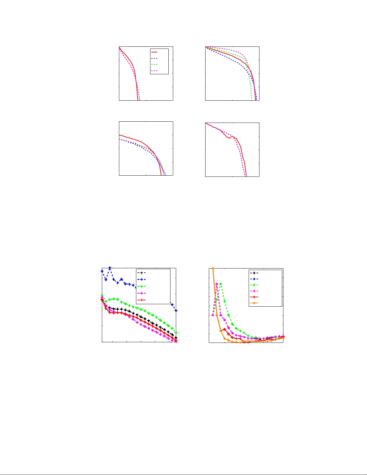
SPECTRAL RANKING USING SERIA TION F AJWEL FOGEL, ALEXANDRE D’ASPREMONT, AND MILAN V OJNO VIC A B S T R AC T . W e describe a seriation algorithm for ranking a set of items given pairwise comparisons between these items. Intuitively , the algorithm assigns similar rankings to items that compare similarly with all others. It does so by constructing a similarity matrix from pairwise comparisons, using seriation methods to reorder this matrix and construct a ranking. W e first sho w that this spectral seriation algorithm recovers the true ranking when all pairwise comparisons are observed and consistent with a total order . W e then sho w that ranking reconstruction is still exact when some pairwise comparisons are corrupted or missing, and that seriation based spectral ranking is more rob ust to noise than classical scoring methods. Finally , we bound the ranking error when only a random subset of the comparions are observed. An additional benefit of the seriation formulation is that it allo ws us to solve semi-supervised ranking problems. Experiments on both synthetic and real datasets demonstrate that seriation based spectral ranking achie ves competiti ve and in some cases superior performance compared to classical ranking methods. 1. I N T RO D U C T I O N W e study the problem of ranking a set of n items given pairwise comparisons between these items 1 . The problem of aggregating binary relations has been formulated more than two centuries ago, in the context of emerging social sciences and voting theories [ de Borda , 1781 ; de Condorcet , 1785 ]. The setting we study here goes back at least to [ Zermelo , 1929 ; Kendall and Smith , 1940 ] and seeks to reconstruct a ranking of items from pairwise comparisons reflecting a total ordering. In this case, the directed graph of all pairwise comparisons, where ev ery pair of vertices is connected by exactly one of two possible directed edges, is usually called a tournament graph in the theoretical computer science literature or a “round robin” in sports, where ev ery player plays e very other player once and each preference marks victory or defeat. The mo- ti vation for this formulation often stems from the fact that in many applications, e.g. music, images, and movies, preferences are easier to e xpress in relati ve terms (e.g. a is better than b ) rather than absolute ones (e.g. a should be ranked fourth, and b se venth). In practice, the information about pairwise comparisons is usually incomplete , especially in the case of a large set of items, and the data may also be noisy , that is some pairwise comparisons could be incorrectly measured and inconsistent with a total order . Ranking is a classical problem b ut its formulations vary widely . In particular , assumptions about how the pairwise preference information is obtained vary a lot from one reference to another . A subset of preferences is measured adaptiv ely in [ Ailon , 2011 ; Jamieson and Nowak , 2011 ], while [ Freund et al. , 2003 ; Negahban et al. , 2012 ] extract them at random. In other settings, the full preference matrix is observ ed, b ut is perturbed by noise: in e.g. [ Bradley and T erry , 1952 ; Luce , 1959 ; Herbrich et al. , 2006 ], a parametric model is assumed ov er the set of permutations, which reformulates ranking as a maximum likelihood problem. Loss functions, performance metrics and algorithmic approaches vary as well. K enyon-Mathieu and Schudy [ 2007 ], for example, deri ve a PT AS for the minimum feedback arc set problem on tournaments, i.e. the problem of finding a ranking that minimizes the number of upsets (a pair of players where the player ranked lo wer on the ranking beats the player ranked higher). In practice, the complexity of this method is relati vely high, and other authors [see e.g. K eener , 1993 ; Neg ahban et al. , 2012 ] ha ve been using spectral Date : September 17, 2018. 2010 Mathematics Subject Classification. 62F07, 06A07, 90C27. K ey wor ds and phrases. Ranking, seriation, spectral methods. 1 A subset of these results appeared at NIPS 2014. 1 methods to produce more efficient algorithms (each pairwise comparison is understood as a link pointing to the preferred item). In other cases, such as the classical Analytic Hierarchy Process (AHP) [ Saaty , 1980 ; Barbeau , 1986 ] preference information is encoded in a “reciprocal” matrix whose Perron-Frobenius eigen- vector pro vides the global ranking. Simple scoring methods such as the point difference rule [ Huber , 1963 ; W authier et al. , 2013 ] produce efficient estimates at very lo w computational cost. W ebsite ranking methods such as PageRank [ Page et al. , 1998 ] and HITS [ Kleinberg , 1999 ] seek to rank web pages based on the hyper- link structure of the web, where links do not necessarily express consistent preference relationships (e.g. a can link to b and b can link c , and c can link to a ). [ Negahban et al. , 2012 ] adapt the PageRank ar gument to the ranking from pairwise comparisons and V igna [ 2009 ] provides a re vie w of ranking algorithms gi ven pairwise comparisons, in particular those in volving the estimation of the stationary distrib ution of a Markov chain. Ranking has also been approached as a prediction problem, i.e. learning to rank [ Schapire et al. , 1998 ; Rajkumar and Agarwal , 2014 ], with [ Joachims , 2002 ] for e xample using support vector machines to learn a score function. Finally , in the Bradley-T erry-Luce framework, where multiple observations on pair- wise preferences are observed and assumed to be generated by a generalized linear model, the maximum likelihood problem is usually solved using fixed point algorithms or EM-like majorization-minimization techniques [ Hunter , 2004 ]. Jiang et al. [ 2011 ] describes the HodgeRank algorithm, which formulates rank- ing given pairwise comparisons as a least-square problem. This formulation is based on Hodge theory and provides tools to measure the consistency of a set of pairwise comparisons with the existence of a global ranking. Duchi et al. [ 2010 , 2013 ] analyze the consistency of various ranking algorithms gi ven pairwise comparisons and a query . Preferences are aggregated through standard procedures, e.g., computing the mean of comparisons from dif ferent users, then ranking are deri ved using classical algorithms, e.g., Borda Count, Bradley-T erry-Model maximum likelihood estimation, least squares, odd-ratios [ Saaty , 2003 ]. Here, we sho w that the ranking problem is directly related to another classical ordering problem, namely seriation . Gi ven a similarity matrix between a set of n items and assuming that the items can be ordered along a chain (path) such that the similarity between items decreases with their distance within this chain (i.e. a total order exists), the seriation problem seeks to reconstruct the underlying linear ordering based on unsorted, possibly noisy , pairwise similarity information. Atkins et al. [ 1998 ] produced a spectral algorithm that exactly solves the seriation problem in the noiseless case, by showing that for similarity matrices com- puted from serial v ariables, the ordering of the eigen vector corresponding to the second smallest eigen v alue of the Laplacian matrix (a.k.a. the Fiedler vector) matches that of the variables. In practice, this means that performing spectral ordering on the similarity matrix exactly reconstructs the correct ordering pro vided items are org anized in a chain. W e adapt these results to ranking to produce a very efficient spectral ranking algorithm with pro vable r ecovery and r obustness guarantees . Furthermore, the seriation formulation allows us to handle semi- supervised ranking problems. Fogel et al. [ 2013 ] sho w that seriation is equiv alent to the 2-SUM problem and study con vex relaxations to seriation in a semi-supervised setting, where additional structural constraints are imposed on the solution. Sev eral authors [ Blum et al. , 2000 ; Feige and Lee , 2007 ] have also focused on the directly related Minimum Linear Arrangement (MLA) problem, for which excellent approximation guarantees exist in the noisy case, albeit with v ery high polynomial complexity . The main contributions of this paper can be summarized as follows. W e link seriation and ranking by sho wing ho w to construct a consistent similarity matrix based on consistent pairwise comparisons. W e then reco ver the true ranking by applying the spectral seriation algorithm in [ Atkins et al. , 1998 ] to this similarity matrix (we call this method SerialRank in what follows). In the noisy case, we then show that spectral seriation can perfectly recov er the true ranking e ven when some of the pairwise comparisons are either corrupted or missing, provided that the pattern of errors is somewhat unstructured. W e show in particular that, in a regime where a high proportion of comparisons are observed, some incorrectly , the spectral solution is more robust to noise than classical scoring based methods. On the other hand, when only few comparisons are observed, we sho w that for Erd ¨ os-R ´ enyi graphs, i.e., when pairwise comparisons are observed independently with a giv en probability , Ω( n log 4 n ) comparisons suf fice for ` 2 consistency 2 of the Fiedler vector and hence ` 2 consistency of the retreived ranking w .h.p. On the other hand we need Ω( n 3 / 2 log 4 n ) comparisons to retrieve a ranking whose local perturbations are bounded in ` ∞ norm. Since for Erd ¨ os-R ´ enyi graphs the induced graph of comparisons is connected with high probability only when the total number of pairs sampled scales as Ω( n log n ) (aka the coupon collector ef fect), we need at least that many comparisons in order to retriev e a ranking, therefore the ` 2 consistency result can be seen as optimal up to a polylog arithmic factor . Finally , we use the seriation results in [ Fogel et al. , 2013 ] to produce semi-supervised ranking solutions. The paper is or ganized as follo ws. In Section 2 we recall definitions related to seriation, and link ranking and seriation by showing ho w to construct well ordered similarity matrices from well ranked items. In Section 3 we apply the spectral algorithm of [ Atkins et al. , 1998 ] to reorder these similarity matrices and reconstruct the true ranking in the noiseless case. In Section 4 we then show that this spectral solution remains exact in a noisy regime where a random subset of comparisons is corrupted. In Section 5 we analyze ranking perturbation results when only fe w comparisons are gi ven following an Erd ¨ os-R ´ enyi graph. Finally , in Section 6 we illustrate our results on both synthetic and real datasets, and compare ranking performance with classical MLE, spectral and scoring based approaches. 2. S E R I A T I O N , S I M I L A R I T I E S & R A N K I N G In this section we first introduce the seriation problem, i.e. reordering items based on pairwise similarities. W e then show ho w to write the problem of ranking gi ven pairwise comparisons as a seriation problem. 2.1. The Seriation Problem. The seriation problem seeks to reorder n items given a similarity matrix between these items, such that the more similar two items are, the closer the y should be. This is equi valent to supposing that items can be placed on a chain where the similarity between two items decreases with the distance between these items in the chain. W e formalize this belo w , follo wing [ Atkins et al. , 1998 ]. Definition 2.1. W e say that a matrix A ∈ S n is an R-matrix (or Robinson matrix) if and only if it is symmetric and A i,j ≤ A i,j +1 and A i +1 ,j ≤ A i,j in the lower triangle, wher e 1 ≤ j < i ≤ n . Another way to formulate R-matrix conditions is to impose A ij ≥ A kl if | i − j | ≤ | k − l | off-diagonal, i.e. the coefficients of A decrease as we move a way from the diagonal. W e also introduce a definition for strict R-matrices A , whose ro ws and columns cannot be permuted without breaking the R-matrix monotonic- ity conditions. W e call re verse identity permutation the permutation that puts rows and columns 1 , 2 , . . . , n of a matrix A in reverse order n, n − 1 , . . . , 1 . Definition 2.2. An R-matrix A ∈ S n is called strict-R if and only if the identity and re verse identity permu- tations of A are the only permutations r eor dering A as an R-matrix. Any R-matrix with only strict R-constraints is a strict R-matrix. F ollowing [ Atkins et al. , 1998 ], we will say that A is pr e-R if there is a permutation matrix Π such that Π A Π T is an R-matrix. Gi ven a pre-R matrix A , the seriation problem consists in finding a permutation Π such that Π A Π T is an R-matrix. Note that there might be sev eral solutions to this problem. In particular , if a permutation Π is a solution, then the re verse permutation is also a solution. When only two permutations of A produce R-matrices, A will be called pr e-strict-R . 2.2. Constructing Similarity Matrices from Pairwise Comparisons. Giv en an ordered input pairwise comparison matrix, we now show how to construct a similarity matrix which is strict-R when all comparisons are gi ven and consistent with the identity ranking (i.e., items are ranked in increasing order of indices). This means that the similarity between two items decreases with the distance between their ranks. W e will then be able to use the spectral seriation algorithm by [ Atkins et al. , 1998 ] described in Section 3 to reconstruct the true ranking from a disordered similarity matrix. W e first show how to compute a pairwise similarity from pairwise comparisons between items by counting the number of matching comparisons. Another formulation allows us to handle the generalized linear model. 3 These two e xamples are only two particular instances of a broader class of ranking algorithms deri ved here. Any method which produces R-matrices from pairwise preferences yields a v alid ranking algorithm. 2.2.1. Similarities fr om P airwise Comparisons. Suppose we are giv en a matrix of pairwise comparisons C ∈ {− 1 , 0 , 1 } n × n such that C i,j = − C j,i for e very i 6 = j and C i,j =    1 if i is ranked higher than j 0 if i and j are not compared or in a draw − 1 if j is ranked higher than i (1) setting C i,i = 1 for all i ∈ { 1 , . . . , n } . W e define the pairwise similarity matrix S match as S match i,j = n X k =1  1 + C i,k C j,k 2  . (2) Since C i,k C j,k = 1 , if C i,k and C j,k hav e matching signs, and C i,k C j,k = − 1 if they have opposite signs, S match i,j counts the number of matching comparisons between i and j with other reference items k . If i or j is not compared with k , then C i,k C j,k = 0 and the term (1 + C i,k C j,k ) / 2 has an neutral ef fect on the similarity of 1 / 2 . Note that we also have S match = 1 2  n 11 T + C C T  . (3) The intuition behind the similarity S match is easy to understand in a tournament setting: players that beat the same players and are beaten by the same players should hav e a similar ranking. The next result shows that when all comparisons are given and consistent with the identity ranking, then the similarity matrix S match is a strict R-matrix. W ithout loss of generality , we assume that items are ranked in increasing order of their indices. In the general case, we can simply replace the strict-R property by the pr e-strict-R property . Proposition 2.3. Given all pairwise comparisons between items ranked accor ding to the identity permuta- tion (with no ties), the similarity matrix S match constructed in ( 2 ) is a strict R-matrix and S match i,j = n − | i − j | (4) for all i, j = 1 , . . . , n . Proof . Since items are ranked as 1 , 2 , . . . , n with no ties and all comparisons gi ven, C i,j = − 1 if i < j and C i,j = 1 otherwise. Therefore we obtain from definition ( 2 ) S match i,j = min( i,j ) − 1 X k =1  1 + 1 2  + max( i,j ) − 1 X k =min( i,j )  1 − 1 2  + n X k =max( i,j )  1 + 1 2  = n − (max( i, j ) − min( i, j )) = n − | i − j | This means in particular that S match is strictly positiv e and its coefficients are strictly decreasing when moving a way from the diagonal, hence S match is a strict R-matrix. 2.2.2. Similarities in the Generalized Linear Model. Suppose that paired comparisons are generated ac- cording to a generalized linear model (GLM), i.e., we assume that the outcomes of paired comparisons are independent and for an y pair of distinct items, item i is observed rank ed higher than item j with probability P i,j = H ( ν i − ν j ) (5) where ν ∈ R n is a vector of skill parameters and H : R → [0 , 1] is a function that is increasing on R and such that H ( − x ) = 1 − H ( x ) for all x ∈ R , and lim x →−∞ H ( x ) = 0 and lim x →∞ H ( x ) = 1 . A 4 well kno wn special instance of the generalized linear model is the Bradley-T erry-Luce model for which H ( x ) = 1 / (1 + e − x ) , for x ∈ R . Let m i,j be the number of times items i and j were compared, C s i,j ∈ {− 1 , 1 } be the outcome of com- parison s and Q be the matrix of corresponding sample probabilities, i.e. if m i,j > 0 we ha ve Q i,j = 1 m i,j m i,j X s =1 C s i,j + 1 2 and Q i,j = 1 / 2 in case m i,j = 0 . W e define the similarity matrix S glm from the observ ations Q as S glm i,j = n X k =1 1 { m i,k m j,k > 0 } (1 − | Q i,k − Q j,k | ) + 1 { m i,k m j,k =0 } 2 . (6) Since the comparison observations are independent we hav e that Q i,j con verges to P i,j as m i,j goes to infinity and the central limit theorem implies that S glm i,j con verges to a Gaussian v ariable with mean n X k =1 (1 − | P i,k − P j,k | ) . The result below shows that this limit similarity matrix is a strict R-matrix when items are properly ordered. Proposition 2.4. If items are or der ed according to the or der in decreasing values of the skill parameters, the similarity matrix S glm is a strict R matrix with high pr obability as the number of observations goes to infinity . Proof . Without loss of generality , we suppose the true order is 1 , 2 , . . . , n , with ν (1) > . . . > ν ( n ) . For any i, j, k such that i > j , using the GLM assumption (i) we get P i,k = H ( ν ( i ) − ν ( k )) < H ( ν ( j ) − ν ( k )) = P j,k . Since empirical probabilities Q i,j con verge to P i,j , when the number of observ ations is large enough, we also ha ve Q i,k < Q j,k for an y i, j, k such that i > j (we focus w .l.o.g. on the lo wer triangle), and we can therefore remov e the absolute value in the e xpression of S glm i,j for i > j . Hence for any i > j we hav e S glm i +1 ,j − S glm i,j = − n X k =1 | Q i +1 ,k − Q j,k | + n X k =1 | Q i,k − Q j,k | = n X k =1 ( Q i +1 ,k − Q j,k ) − ( Q i,k − Q j,k ) = n X k =1 Q i +1 ,k − Q i,k < 0 . Similarly for any i > j , S glm i,j − 1 − S glm i,j < 0 , so S glm is a strict R-matrix. Notice that we recover the original definition of S match in the case of binary comparisons, though it does not fit in the Generalized Linear Model. Note also that these definitions can be directly extended to the setting where multiple comparisons are av ailable for each pair and aggreg ated in comparisons that take fractional v alues (e.g., a tournament setting where participants play sev eral times against each other). 3. S P E C T R A L A L G O R I T H M S W e first recall how spectral ordering can be used to recover the true ordering in seriation problems. W e then apply this method to the ranking problem. 5 3.1. Spectral Seriation Algorithm. W e use the spectral computation method originally introduced in [ Atkins et al. , 1998 ] to solv e the seriation problem based on the similarity matrices defined in the previ- ous section. W e first recall the definition of the Fiedler v ector (which is sho wn to be unique in our setting in Lemma 3.3 ). Definition 3.1. The F iedler value of a symmetric, nonne gative and irr educible matrix A is the smallest non-zer o eigen value of its Laplacian matrix L A = diag ( A 1 ) − A . The corr esponding eigen vector is called F iedler vector and is the optimal solution to min { y T L A y : y ∈ R n , y T 1 = 0 , k y k 2 = 1 } . The main result from [ Atkins et al. , 1998 ], detailed belo w , sho ws ho w to reorder pre-R matrices in a noise free case. Proposition 3.2. [ Atkins et al. , 1998 , Th. 3.3] Let A ∈ S n be an irreducible pre-R-matrix with a simple F iedler value and a F iedler vector v with no r epeated values. Let Π 1 ∈ P (r espectively , Π 2 ) be the per- mutation such that the permuted F iedler vector Π 1 v is strictly incr easing (decr easing). Then Π 1 A Π T 1 and Π 2 A Π T 2 ar e R-matrices, and no other permutations of A pr oduce R-matrices. The next technical lemmas extend the results in Atkins et al. [ 1998 ] to strict R-matrices and will be used to prove Theorem 3.6 in next section. The first one sho ws that without loss of generality , the Fiedler v alue is simple. Lemma 3.3. If A is an irr educible R-matrix, up to a uniform shift of its coefficients, A has a simple F iedler value and a monotonic F iedler vector . Proof . W e use [ Atkins et al. , 1998 , Th. 4.6] which states that if A is an irreducible R-matrix with A n, 1 = 0 , then the Fiedler value of A is a simple eigen value. Since A is an R-matrix, A n, 1 is among its minimal elements. Subtracting it from A does not af fect the nonnegati vity of A and we can apply [ Atkins et al. , 1998 , Th. 4.6]. Monotonicity of the Fiedler vector then follo ws from [ Atkins et al. , 1998 , Th. 3.2]. The next lemma sho ws that the Fiedler vector is strictly monotonic if A is a strict R-matrix. Lemma 3.4. Let A ∈ S n be an irreducible R-matrix. Suppose there ar e no distinct indices r < s such that for any k 6∈ [ r , s ] , A r,k = A r +1 ,k = . . . = A s,k , then, up to a uniform shift, the F iedler value of A is simple and its F iedler vector is strictly monotonic. Proof . By Lemma 3.3 , the Fiedler value of A is simple (up to a uniform shift of A ). Let x be the corresponding Fiedler vector of A , x is monotonic by Lemma 3.3 . Suppose [ r , s ] is a nontrivial maximal interv al such that x r = x r +1 = . . . = x s , then by [ Atkins et al. , 1998 , lemma 4.3], for any k 6∈ [ r , s ] , A r,k = A r +1 ,k = . . . = A s,k , which contradicts the initial assumption. Therefore x is strictly monotonic. In fact, we only need a small portion of the R-constraints to be strict for the previous lemma to hold. W e no w show that the main assumption on A in Lemma 3.4 is equiv alent to A being strict-R. Lemma 3.5. An irreducible R-matrix A ∈ S n is strictly R if and only if there ar e no distinct indices r < s such that for any k 6∈ [ r, s ] , A r,k = A r +1 ,k = . . . = A s,k . Proof . Let A ∈ S n an R-matrix. Let us first suppose there are no distinct indices r < s such that for any k 6∈ [ r , s ] , A r,k = A r +1 ,k = . . . = A s,k . By Lemma 3.4 the Fiedler value of A is simple and its Fiedler v ector is strictly monotonic. Hence by Proposition 3.2 , only the identity and reverse identity permutations of A produce R-matrices. No w suppose there e xist tw o distinct indices r < s such that for any k 6∈ [ r, s ] , A r,k = A r +1 ,k = . . . = A s,k . In addition to the identity and re verse identity permutations, we can locally rev erse the order of rows and columns from r to s , since the sub matrix A r : s,r : s is an R-matrix and for any k 6∈ [ r , s ] , A r,k = A r +1 ,k = . . . = A s,k . Therefore at least four different permutations of A produce R-matrices, which means that A is not strictly R. 6 Algorithm 1 (SerialRank) Input: A set of pairwise comparisons C i,j ∈ {− 1 , 0 , 1 } or [ − 1 , 1] . 1: Compute a similarity matrix S as in § 2.2 2: Compute the Laplacian matrix L S = diag ( S 1 ) − S (SerialRank) 3: Compute the Fiedler vector of S . Output: A ranking induced by sorting the Fiedler vector of S (choose either increasing or decreasing order to minimize the number of upsets). 3.2. SerialRank: a Spectral Ranking Algorithm. In Section 2 , we showed that similarities S match and S glm are pr e-strict-R when all comparisons are av ailable and consistent with an underlying ranking of items. W e now use the spectral seriation method in [ Atkins et al. , 1998 ] to reorder these matrices and produce a ranking. Spectral ordering requires computing an extremal eigenv ector , at a cost of O ( n 2 log n ) flops [ Kuczynski and W ozniako wski , 1992 ]. W e call this algorithm SerialRank and prov e the follo wing result. Theorem 3.6. Given all pairwise comparisons for a set of totally or der ed items and assuming ther e are no ties between items, algorithm SerialRank , i.e., sorting the F iedler vector of the matrix S match defined in ( 3 ) , r ecover s the true ranking of items. Proof . From Proposition 2.3 , under assumptions of the proposition S match is a pre-strict R-matrix. No w combining the definition of strict-R matrices in Lemma 3.5 with Lemma 3.4 , we deduce that Fiedler value of S match is simple and its Fiedler vector has no repeated values. Hence by Proposition 3.2 , only the two permutations that sort the Fiedler vector in increasing and decreasing order produce strict R-matrices and are candidate rankings (by Proposition 2.3 S match is a strict R-matrix when ordered according to the true ranking). Finally we can choose between the two candidate rankings (increasing and decreasing) by picking the one with the least upsets. Similar results apply for S glm gi ven enough comparisons in the Generalized Linear Model. This last result guarantees recov ery of the true ranking of items in the noiseless case. In the next section, we will study the impact of corrupted or missing comparisons on the inferred ranking of items. Shift by +1 Shift by -1 i i+1 j j-1 i i+1 j j-1 Strict R-constraints F I G U R E 1 . The matrix of pairwise comparisons C (far left) when the rows are ordered according to the true ranking. The corresponding similarity matrix S match is a strict R- matrix (center left) . The same S match similarity matrix with comparison (3,8) corrupted (center right) . W ith one corrupted comparison, S match keeps enough strict R-constraints to recov er the right permutation. In the noiseless case, the difference between all coefficients is at least one and after introducing an error , the coef ficients inside the green rectangles still enforce strict R-constraints (far right) . 7 4. E X A C T R E C OV E RY W I T H C O R R U P T E D A N D M I S S I N G C O M PA R I S O N S In this section we study the robustness of SerialRank using S match with respect to noisy and missing pairwise comparisons. W e will see that noisy comparisons cause ranking ambiguities for the point score method and that such ambiguities are to be lifted by the spectral ranking algorithm. W e sho w in particular that the SerialRank algorithm recovers the exact ranking when the pattern of errors is random and errors are not too numerous. W e first study the impact of one corrupted comparison on SerialRank , then extend the result to multiple corrupted comparisons. A similar analysis is provided for missing comparisons as Corollary 8.3 . in the Appendix. Finally , Proposition 4.4 provides an estimate of the number of randomly corrupted entries that can be tolerated for perfect recovery of the true ranking. W e begin by recalling the definition of the point scor e of an item. Definition 4.1. The point score w i of an item i , also known as point-differ ence, or row-sum is defined as w i = P n k =1 C k,i , whic h corresponds to the number of wins minus the number of losses in a tournament setting. In the follo wing we will denote by w the point score v ector . Proposition 4.2. Given all pairwise comparisons C s,t ∈ {− 1 , 1 } between items rank ed according to their indices, suppose the sign of one comparison C i,j (and its counterpart C j,i ) is switched, with i < j . If j − i > 2 then S match defined in ( 3 ) r emains strict-R , wher eas the point scor e vector w has ties between items i and i + 1 and items j and j − 1 . Proof . W e gi ve some intuition for the result in Figure 1 . W e write the true score and comparison matrix w and C , while the observ ations are written ˆ w and ˆ C respectively . This means in particular that ˆ C i,j = − C i,j = 1 and ˆ C j,i = − C j,i = − 1 . T o simplify notations we denote by S the similarity matrix S match (respecti vely ˆ S when the similarity is computed from observ ations). W e first study the impact of a corrupted comparison C i,j for i < j on the point score vector ˆ w . W e ha ve ˆ w i = n X k =1 ˆ C k,i = n X k =1 C k,i + ˆ C j,i − C j,i = w i − 2 = w i +1 , similarly ˆ w j = w j − 1 , whereas ˆ w k = w k for k 6 = i, j . Hence, the incorrect comparison induces two ties in the point score v ector w . No w we show that the similarity matrix defined in ( 3 ) breaks these ties, by sho wing that it is a strict R-matrix. Writing ˆ S in terms of S , we get for any t 6 = i, j [ ˆ C ˆ C T ] i,t = X k 6 = j  ˆ C i,k ˆ C t,k  + ˆ C i,j ˆ C t,j = X k 6 = j ( C i,k C t,k ) + ˆ C i,j C t,j =  [ C C T ] i,t − 2 if t < j  C C T  i,t + 2 if t > j. Thus we obtain ˆ S i,t =  S i,t − 1 if t < j S i,t + 1 if t > j, (remember there is a factor 1 / 2 in the definition of S ). Similarly we get for any t 6 = i, j ˆ S j,t =  S j,t + 1 if t < i S j,t − 1 if t > i. Finally , for the single corrupted index pair ( i, j ) , we get ˆ S i,j = 1 2   n + X k 6 = i,j  ˆ C i,k ˆ C j,k  + ˆ C i,i ˆ C j,i + ˆ C i,j ˆ C j,j   = S i,j − 1 + 1 = S i,j . The diagonal of S is not impacted since [ ˆ C ˆ C T ] i,i = P n k =1  ˆ C i,k ˆ C i,k  = n . For all other coefficients ( s, t ) such that s, t 6 = i, j , we also have ˆ S s,t = S s,t , which means that all rows or columns outside of i, j are left 8 unchanged. W e first observe that these last equations, together with our assumption that j − i > 2 and the fact that the elements of the e xact S in ( 4 ) differ by at least one, imply that ˆ S s,t ≤ ˆ S s +1 ,t and ˆ S s,t +1 ≤ ˆ S s,t , for s < t so ˆ S remains an R-matrix. Note that this result remains true even when j − i = 2 , b ut we need some strict inequalities to sho w uniqueness of the retrie ved order . Indeed, because j − i > 2 all these R constraints are strict e xcept between elements of rows i and i + 1 , and ro ws j − 1 and j (and similarly for columns). These ties can be broken using the fact that ˆ S i,j − 1 = S i,j − 1 − 1 < S i +1 ,j − 1 − 1 = ˆ S i +1 ,j − 1 − 1 < ˆ S i +1 ,j − 1 which means that ˆ S is still a strict R-matrix (see Figure 1 ) since j − 1 > i + 1 by assumption. W e now e xtend this result to multiple errors. Proposition 4.3. Given all pairwise comparisons C s,t ∈ {− 1 , 1 } between items rank ed according to their indices, suppose the signs of m comparisons indexed ( i 1 , j 1 ) , . . . , ( i m , j m ) are switched. If the following condition ( 7 ) holds true, | s − t | > 2 , for all s, t ∈ { i 1 , . . . , i m , j 1 , . . . , j m } with s 6 = t, (7) then S match defined in ( 3 ) r emains strict-R , wher eas the point score vector w has 2 m ties. Proof . W e write the true score and comparison matrix w and C , while the observations are written ˆ w and ˆ C respecti vely , and without loss of generality we suppose i l < j l . This implies that ˆ C i l ,j l = − C i l ,j l = 1 and ˆ C j l ,i l = − C j l ,i l = − 1 for all l in { 1 , . . . , m } . T o simplify notations, we denote by S the similarity matrix S match (respecti vely ˆ S when the similarity is computed from observations). As in the proof of Proposition 4.2 , corrupted comparisons index ed ( i l , j l ) induce shifts of ± 1 on columns and rows i l and j l of the similarity matrix S match , while S match i l ,j l v alues remain the same. Since there are se veral corrupted comparisons, we also need to check the values of ˆ S at the intersections of rows and columns with indices of corrupted comparisons. Formally , for any ( i, j ) ∈ { ( i 1 , j 1 ) , . . . ( i m , j m ) } and t 6∈ { i 1 , . . . , i m , j 1 , . . . , j m } ˆ S i,t =  S i,t + 1 if t < j S i,t − 1 if t > j, Similarly for t 6∈ { i 1 , . . . , i m , j 1 , . . . , j m } ˆ S j,t =  S j,t − 1 if t < i S j,t + 1 if t > i. Let ( s, s 0 ) and ( t, t 0 ) ∈ { ( i 1 , j 1 ) , . . . ( i m , j m ) } , we hav e ˆ S s,t = 1 2  n + P k 6 = s 0 ,t 0  ˆ C s,k ˆ C t,k  + ˆ C s,s 0 ˆ C t,s 0 + ˆ C s,t 0 ˆ C t,t 0  = 1 2  n + P k 6 = s 0 ,t 0 ( C s,k C t,k ) − C s,s 0 C t,s 0 − C s,t 0 C t,t 0  W ithout loss of generality we suppose s < t , and since s < s 0 and t < t 0 , we obtain ˆ S s,t =  S s,t if t > s 0 S s,t + 2 if t < s 0 . Similar results apply for other intersections of rows and columns with indices of corrupted comparisons (i.e., shifts of 0 , +2 , or − 2 ). For all other coefficients ( s, t ) such that s, t 6∈ { i 1 , . . . , i m , j 1 , . . . , j m } , we hav e ˆ S s,t = S s,t . W e first observe that these last equations, together with our assumption that j l − i l > 2 , mean that ˆ S s,t ≤ ˆ S s +1 ,t and ˆ S s,t +1 ≤ ˆ S s,t , for any s < t 9 so ˆ S remains an R-matrix. Moreover , since j l − i l > 2 all these R constraints are strict except between elements of ro ws i l and i l + 1 , and ro ws j l − 1 and j l (similar for columns). These ties can be broken using the fact that for k = j l − 1 ˆ S i l ,k = S i l ,k − 1 < S i l +1 ,k − 1 = ˆ S i l +1 ,k − 1 < ˆ S i l +1 ,k which means that ˆ S is still a strict R-matrix since k = j l − 1 > i l + 1 . Moreover , using the same argument as in the proof of Proposition 4.2 , corrupted comparisons induces 2 m ties in the point score vector w . For the case of one corrupted comparison, note that the separation condition on the pair of items ( i, j ) is necessary . When the comparison C i,j between two adjacent items is corrupted, no ranking method can break the resulting tie. For the case of arbitrary number of corrupted comparisons, condition ( 7 ) is a sufficient condition only . W e study e xact ranking recovery conditions with missing comparisons in the Appendix, using similar arguments. W e no w estimate the number of randomly corrupted entries that can be tolerated while maintaining exact reco very of the true ranking. Proposition 4.4. Given a comparison matrix for a set of n items with m corrupted comparisons selected uniformly at random fr om the set of all possible item pairs. Algorithm SerialRank guarantees that the pr obability of reco very p ( n, m ) satisfies p ( n, m ) ≥ 1 − δ , pr ovided that m = O ( √ δ n ) . In particular , this implies that p ( n, m ) = 1 − o (1) pro vided that m = o ( √ n ) . Proof . Let P be the set of all distinct pairs of items from the set { 1 , 2 , . . . , n } . Let X be the set of all admissible sets of pairs of items, i.e. containing each X ⊆ P such that X satisfies condition ( 7 ). W e consider the case of m ≥ 1 distinct pairs of items sampled from the set P uniformly at random without replacement. Let X i denote the set of sampled pairs giv en that i pairs are sampled. W e seek to bound p ( n, m ) = Prob ( X m ∈ X ) . Gi ven a set of pairs X ∈ X , let T ( X ) be the set of non-admissible pairs, i.e. containing ( i, j ) ∈ P \ X such that X ∪ ( i, j ) / ∈ X . W e have Prob ( X m ∈ X ) = X x ∈X : | x | = m − 1  1 − | T ( x ) | |P | − ( m − 1)  Prob ( X m − 1 = x ) . (8) Note that e very selected pair from P contributes at most 15 n non-admissible pairs. Indeed, giv en a selected pair ( i, j ) , a non-admissible pair ( s, t ) should respect one of the following conditions | s − i | ≤ 2 , | s − j | ≤ 2 , | t − i | ≤ 2 , | t − j | ≤ 2 or | s − t | ≤ 2 . Giv en any item s , there are 15 possible choice of t to output a non- admissible pair ( s, t ) , resulting in at most 15 n non-admissible pairs for the selected pair ( i, j ) . Hence, for e very x ∈ X we hav e | T ( x ) | ≤ 15 n | x | . Combining this with ( 8 ) and the fact that |P | =  n 2  , we hav e Prob ( X m ∈ X ) ≥ 1 − 15 n  n 2  − ( m − 1) ( m − 1) ! Prob ( X m − 1 ∈ X ) . From this it follo ws p ( n, m ) ≥ m − 1 Y i =1 1 − 15 n  n 2  − ( i − 1) i ! ≥ m − 1 Y i =1  1 − i a ( n, m )  where a ( n, m ) =  n 2  − ( m − 1) 15 n . 10 Notice that when m = o ( n ) we ha ve  1 − i a ( n,m )  ∼ exp( − 30 i/n ) and m − 1 Y i =1  1 − i a ( n, m )  ∼ m − 1 Y i =1 exp( − 30 i/n ) ∼ exp  − 15 m 2 n  for large n. Hence, given δ > 0 , p ( n, m ) ≥ 1 − δ provided that m = O ( √ nδ ) . If δ = o (1) , the condition is m = o ( √ n ) . 5. S P E C T R A L P E RT U R B A T I O N A N A LY S I S In this section we analyze how SerialRank performs when only a small fraction of pairwise comparisons are gi ven. W e sho w that for Erd ¨ os-R ´ enyi graphs, i.e., when pairwise comparisons are observed indepen- dently with a gi ven probability , Ω( n log 4 n ) comparisons suf fice for ` 2 consistency of the Fiedler vector and hence ` 2 consistency of the retreiv ed ranking w .h.p. On the other hand we need Ω( n 3 / 2 log 4 n ) comparisons to retrie ve a ranking whose local perturbations are bounded in ` ∞ norm. Since Erd ¨ os-R ´ enyi graphs are connected with high probability only when the total number of pairs sampled scales as Ω( n log n ) , we need at least that many comparisons in order to retrie ve a ranking, therefore the ` 2 consistency result can be seen as optimal up to a polylogarithmic factor . Our bounds are mostly related to the work of [ W authier et al. , 2013 ]. In its simplified version [Theorem 4.2 W authier et al. , 2013 ] shows that when ranking items according to their point score, for any precision parameter µ ∈ (0 , 1) , sampling independently with fixed probability Ω  n log n µ 2  comparisons guarantees that the maximum displacement between the retriev ed ranking and the true ranking, i.e., the ` ∞ distance to the true ranking, is bounded by µn with high probability for n large enough. Sample comple xity bounds hav e also been studied for the Rank Centrality algorithm [ Dw ork et al. , 2001 ; Negahban et al. , 2012 ]. In their analysis, [ Negahban et al. , 2012 ] suppose that some pairs are sampled independently with fixed probability , and then k comparisons are generated for each sampled pair , under a Bradley-T erry-Luce model (BTL). When ranking items according to the stationary distribution of a transition matrix estimated from comparisons, sampling Ω( n · polylog ( n )) pairs are enough to bound the relati ve ` 2 norm perturbation of the stationary distribution. Ho we ver , as pointed out by [ W authier et al. , 2013 ], repeated measurements are not practical, e.g., if comparisons are deri ved from the outcomes of sports games or the purchasing beha vior of a customer (a customer typically wants to purchase a product only once). Moreover , [ Negahban et al. , 2012 ] do not pro vide bounds on the relati ve ` ∞ norm perturbation of the ranking. W e also refer the reader to the recent work of Rajkumar and Agarwal [ 2014 ], who provide a survey of sample complexity bounds for Rank Centrality , maximum likelihood estimation, least-square ranking and an SVM based ranking, under a more flexible sampling model. Howe ver , those bounds only give the sampling complexity for e xact recovery of ranking, which is usually prohibitiv e when n is lar ge, and are more dif ficult to interpret. Finally , we refer the interested reader to [ Huang et al. , 2008 ; Shamir and Tishby , 2011 ] for sampling complexity bounds in the conte xt of spectral clustering. Limitations. W e emphasize that sampling models based on Erd ¨ os-R ´ enyi graphs are not the most realistic, though they ha ve been studied widely in the literature [see for instance Feige et al. , 1994 ; Brav erman and Mossel , 2008 ; W authier et al. , 2013 ]. Indeed, pairs are not lik ely to be sampled independently . For instance, when ranking movies, popular movies in the top ranks are more likely to be compared. Corrupted com- parisons are also more likely between items that hav e close rankings. W e hope to extend our perturbation analysis to more general models in future work. A second limitation of our perturbation analysis comes from the setting of ordinal comparisons, i.e., binary comparisons, since in many applications, se veral comparisons are provided for each sampled pair . Ne vertheless, the setting of ordinal comparisons is interesting for the analysis of SerialRank , since numerical 11 experiments suggest that it is the setting for which SerialRank provides the best results compared to other methods. Note that in practice, we can easily get rid of this limitation (see Section 2.2.2 and 6 ). W e refer the reader to numerical experiments in Section 6 , as well as a recent paper by Cucuringu [ 2015 ], which introduces another ranking algorithm called SyncRank, and provides extensi ve numerical experiments on state-of-the-art ranking algorithms, including SerialRank . Choice of Laplacian: normalized vs. unnormalized. In the spectral clustering literature, sev eral con- structions for the Laplacian operators are suggested, namely the unnormalized Laplacian (used in Serial- Rank ), the symmetric normalized Laplacian, and the non-symmetric normalized Laplacian. V on Luxburg et al. [ 2008 ] sho w stronger consistenc y results for spectral clustering by using the non-symmetric normal- ized Laplacian. Here, we sho w that the Fiedler vector of the normalized Laplacian is an affine function of the ranking, hence sorting the Fiedler vector still guarantees exact recovery of the ranking, when all compar- isons are observed and consistent with a global ranking. In contrast, we only get an asymptotic expression for the unnormalized Laplacian ( cf . section 8 ). This motiv ated us to provide an analysis of SerialRank ro- bustness based on the normalized Laplacian, though in practice the use of the unnormalized Laplacian is v alid and seems to giv e better results ( cf. Figures 2 and 5 ). Notations. Throughout this section, we only focus on the similarity S match in ( 3 ) and write it S to simplify notations. W .l.o.g. we assume in the following that the true ranking is the identity , hence S is an R-matrix. W e write k · k 2 the operator norm of a matrix, which corresponds to the maximal absolute eigen value for symmetric matrices. k · k F denotes the Frobenius norm. W e refer to the eigen values of the Laplacian as λ i , with λ 1 = 0 ≤ λ 2 ≤ . . . ≤ λ n . For any quantity x , we denote by ˜ x its perturbed analogue. W e define the residual matrix R = ˜ S − S and write f the normalized Fiedler v ector of the Laplacian matrix L S . W e define the degree matrix D S = diag ( D 1 ) the diagonal matrix whose elements are the ro w-sums of matrix S . Whene ver we use the abreviation w .h.p., this means that the inequality is true with probability greater than 1 − 2 /n . Finally , we will use c > 0 for absolute constants, whose values are allowed to vary from one equation to another . W e assume that our information on preferences is both incomplete and corrupted. Specifically , pairwise comparisons are independently sampled with probability q and these sampled comparisons are consistent with the underlying total ranking with probability p . Let us define ˜ C = B ◦ C the matrix of observed comparisons, where C is the true comparison matrix defined in ( 1 ), ◦ is the Hadamard product and B is a symmetric matrix with entries B i,j =    0 with probability 1 − q 1 with probability q p − 1 with probability q (1 − p ) . In order to obtain an unbiased estimator of the comparison matrix defined in ( 1 ), we normalize ˜ C by its mean v alue q (2 p − 1) and redefine ˜ S as ˜ S = 1 q 2 (2 p − 1) 2 ˜ C ˜ C T + n 11 T . For ease of notations we hav e dropped the factor 1 / 2 in ( 3 ) w .l.o.g. (positiv e multiplicativ e factors of the Laplacian do not af fect its eigen vectors). 5.1. Results. W e no w state our main results. The first one bounds ` 2 perturbations of the Fiedler v ector f with both missing and corrupted comparisons. Note that f and ˜ f are normalized. Theorem 5.7 . F or every µ ∈ (0 , 1) and n lar ge enough, if q > log 4 n µ 2 (2 p − 1) 4 n , then k ˜ f − f k 2 ≤ c µ √ log n with pr obability at least 1 − 2 /n , wher e c > 0 is an absolute constant. 12 As n goes to infinity the perturbation of the Fiedler vector goes to zero, and we can retrieve the “true” ranking by reordering the Fiedler vector . Hence this bounds provides ` 2 consistency of the ranking, with an optimal sampling complexity (up to a polylogarithmic f actor). The second result bounds local perturbations of the ranking with π referring to the “true” ranking and ˜ π to the ranking retrie ved by SerialRank . Theorem 5.10 . F or every µ ∈ (0 , 1) and n lar ge enough, if q > log 4 n µ 2 (2 p − 1) 4 √ n , then k ˜ π − π k ∞ ≤ cµn with pr obability at least 1 − 2 /n , wher e c > 0 is an absolute constant. This bound quantifies the maximum displacement of any item’ s ranking. µ can be seen a “precision” parameter . For instance, if we set µ = 0 . 1 , Theorem 5.10 means that we can e xpect the maximum displace- ment of an y item’ s ranking to be less than 0 . 1 · n when observing c 2 · 100 · n √ n · log 4 n comparisons (with p = 1 ). W e conjecture Theorem 5.10 still holds true if the condition q > log 4 n/µ 2 (2 p − 1) 4 √ n is replaced by the weaker condition q > log 4 n/µ 2 (2 p − 1) 4 n . 5.2. Sketch of the proof . The proof of these results relies on classical perturbation arguments and is struc- tured as follo ws. • Step 1: Bound k ˜ D S − D S k 2 , k ˜ S − S k 2 with high probability using concentration inequalities on quadratic forms of Bernoulli v ariables and results from [ Achlioptas and McSherry , 2007 ]. • Step 2. Show that the normalized Laplacian L = I − D − 1 S has a linear Fiedler vector and bound the eigengap between the Fiedler v alue and other eigen v alues. • Step 3. Bound k ˜ f − f k 2 using Davis-Kahan theorem and bounds of steps 1 and 2. • Step 4. Use the linearity of the Fiedler vector to translate this result into a bound on the maximum displacement of the retrie ved ranking k ˜ π − π k ∞ . W e now turn to the proof itself. 5.3. Step 1: Bounding k ˜ D S − D S k 2 and k ˜ S − S k 2 . Here, we seek to bound k ˜ D S − D S k 2 and k ˜ S − S k 2 with high probability using concentration inequalities. 5.3.1. Bounding the norm of the de gr ee matrix. W e first bound perturbations of the degree matrix with both missing and corrupted comparisons. Lemma 5.1. F or every µ ∈ (0 , 1) and n ≥ 100 , if q ≥ log 4 n µ 2 (2 p − 1) 4 n then k ˜ D S − D S k 2 ≤ 3 µn 2 √ log n with pr obability at least 1 − 1 /n . Proof . Let R = ˜ S − S and δ = diag D R = diag (( ˜ S − S ) 1 ) . Since D S and ˜ D S are diagonal matrices, k ˜ D S − D S k 2 = max | δ i | . W e first seek a concentration inequality for each δ i and then deri ve a bound on k ˜ D S − D S k 2 . By definition of the similarity matrix S and its perturbed analogue ˜ S we hav e R ij = n X k =1 C ik C j k  B ik B j k q 2 (2 p − 1) 2 − 1  . Hence δ i = n X j =1 R ij = n X j =1 n X k =1 C ik C j k  B ik B j k q 2 (2 p − 1) 2 − 1  . 13 Notice that we can arbitrarily fix the diagonal v alues of R to zeros. Indeed, the similarity between an element and itself should be a constant by con vention, which leads to R ii = ˜ S ii − S ii = 0 for all items i . Hence we could take j 6 = i in the definition of δ i , and we can consider B ik independent of B j k in the associated summation. W e first seek a concentration inequality for each δ i . Notice that δ i = n X j =1 n X k =1 C ik C j k  B ik B j k q 2 (2 p − 1) 2 − 1  = n X k =1   C ik B ik q (2 p − 1) n X j =1 C j k  B j k q (2 p − 1) − 1    | {z } Quad + n X k =1 n X j =1 C ik C j k  B ik q (2 p − 1) − 1  | {z } Lin . The first term (denoted Quad in the follo wing) is quadratic with respect to the B j k while the second term (denoted Lin in the following) is linear . Both terms hav e mean zero since the B ik are independent of the B j k . W e begin by bounding the quadratic term Quad. Let X j k = C j k  1 q (2 p − 1) B j k − 1  . W e ha ve E ( X j k ) = C j k  q p − q (1 − p ) q (2 p − 1) − 1  = 0 , v ar ( X j k ) = v ar ( B j k ) q 2 (2 p − 1) 2 = 1 q 2 (2 p − 1) 2 ( q − q 2 (2 p − 1) 2 ) = 1 q (2 p − 1) 2 − 1 ≤ 1 q (2 p − 1) 2 , and | X j k | =     B j k q (2 p − 1) − 1     ≤ 1 + 1 q (2 p − 1) ≤ 2 q (2 p − 1) ≤ 2 q (2 p − 1) 2 . By applying Bernstein’ s inequality for any t > 0 Prob         n X j =1 X j k       > t   ≤ 2 exp  − q (2 p − 1) 2 t 2 2( n + 2 t/ 3)  ≤ 2 exp  − q (2 p − 1) 2 t 2 2( n + t )  . (9) No w notice that Prob ( | Quad | > t ) = Prob         n X k =1   C ik B ik q (2 p − 1) n X j =1 X j k         > t   ≤ Prob   n X k =1  | B ik | q (2 p − 1)  max l | n X j =1 X j l | > t   . By applying a union bound to the first Bernstein inequality ( 9 ), for any t > 0 Prob   max l       n X j =1 X j l       > √ t   ≤ 2 n exp  − tq (2 p − 1) 2 2( n + √ t )  . Moreov er , since E | B ik | = q we also get from Bernstein’ s inequality that for any t > 0 Prob n X k =1 | B ik | q (2 p − 1) > n 2 p − 1 + √ t ! ≤ exp  − tq (2 p − 1) 2 2( n + √ t )  . W e deduce from these last three inequalities that for any t > 0 Prob ( | Quad | > t ) ≤ (2 n + 1) exp  − tq (2 p − 1) 2 2( n + √ t )  . 14 T aking t = µ 2 (2 p − 1) 2 n 2 / log n and q ≥ log 4 n µ 2 (2 p − 1) 4 n , with µ ≤ 1 , we hav e √ t ≤ n and we deduce that Prob  | Quad | > 2 µn 2 √ log n  ≤ (2 n + 1) exp  − log 3 n 4  . (10) W e now bound the linear term Lin. Prob ( | Lin | > t ) = Prob         n X j =1 n X k =1 C ik C j k  B ik q (2 p − 1) − 1        > t   ≤ Prob   n X k =1 | C ik | max l | n X j =1 X j l | > t   ≤ Prob   max k | n X j =1 X j k | > t/n   , hence Prob ( | Lin | > t ) ≤ 2 n exp  − t 2 q (2 p − 1) 2 2 n 2 ( n + t/n )  . T aking t = µn 2 / (log n ) 1 / 2 and q ≥ log 4 n µ 2 (2 p − 1) 4 n , with µ ≤ 1 , we hav e t ≤ n 2 and we deduce that Prob ( | Lin | > t ) ≤ 2 n exp  − log 3 n 4  . (11) Finally , combining equations ( 10 ) and ( 11 ), we obtain for q ≥ log 4 n µ 2 (2 p − 1) 4 n , with µ ≤ 1 Prob  | δ i | > 3 µn 2 √ log n  ≤ (4 n + 1) exp  − log 3 n 4  . No w , using a union bound, this shows that for q ≥ log 4 n µ 2 (2 p − 1) 4 n , Prob  max | δ i | > 3 µn 2 √ log n  ≤ n (4 n + 1) exp  − log 3 n 4  , which is less than 1 /n for n ≥ 100 . 5.3.2. Bounding perturbations of the comparison matrix C . Here, we adapt results in [ Achlioptas and Mc- Sherry , 2007 ] to bound perturbations of the comparison matrix. W e will then use bounds on the perturbations of C to bound k ˜ S − S k 2 . Lemma 5.2. F or n ≥ 104 and q ≥ log 3 n n , k C − ˜ C k 2 ≤ c 2 p − 1 r n q , (12) with pr obability at least 1 − 2 /n , wher e c is an absolute constant. Proof . The main argument of the proof is to use the independence of the C ij for i < j in order to bound k ˜ C − C k 2 by a constant times σ √ n , where σ is the standard de viation of C ij . T o isolate independent entries in the perturbation matrix, we first need to break the anti-symmetry of ˜ C − C by decomposing X = ˜ C − C into its upper triangular part and its lower triangular part, i.e., ˜ C − C = X up + X low , with X up = − X T low 15 (diagonal entries of ˜ C − C can be arbitrarily set to 0). Entries of X up are all independent, with v ariance less than the v ariance of ˜ C ij . Indeed, lower entries of X up are equal to 0 and hence ha ve v ariance 0. Notice that k ˜ C − C k 2 = k X up + X low k 2 ≤ k X up k 2 + k X low k 2 ≤ 2 k X up k 2 , so bounding k X up k 2 will gi ve us a bound on k X k 2 . In the rest of the proof we write X up instead of X to simplify notations. W e can no w apply [ Achlioptas and McSherry , 2007 , Th. 3.1] to X . Since X ij = ˜ C ij − C ij = C ij  B ij q (2 p − 1) − 1  , we have ( cf . proof of Lemma 5.1 ) E ( X ij ) = 0 , v ar ( X ij ) ≤ 1 q (2 p − 1) 2 , and | X ij | ≤ 2 q (2 p − 1) . Hence for a gi ven  > 0 such that 4 q (2 p − 1) ≤  log(1 +  ) 2 log (2 n )  2 √ 2 n √ q (2 p − 1) , (13) for any θ > 0 and n ≥ 76 , Prob  k X k 2 ≥ 2(1 +  + θ ) 1 √ q (2 p − 1) √ 2 n  < 2 exp  − 16 θ 2  4 log 3 n  . (14) For q ≥ (log 2 n ) 3 n and taking  ≥ exp( p (16 / p (2))) − 1 (so log (1 +  ) 2 ≥ 16 / √ 2 ) means inequality ( 13 ) holds. T aking ( 14 ) with  = 30 and θ = 30 we get Prob k X k 2 ≥ 2 √ 2(1 + 30 + 30) 2 p − 1 r n q ! < 2 exp  − 10 − 2 log 3 n  . (15) Hence for n ≥ 104 , we hav e log 3 n > 100 and Prob  k X k 2 ≥ 173 2 p − 1 r n q  < 2 /n. Noting that log 2 n ≤ 1 . 15 log n for n ≥ 104 , we obtain the desired result by choosing c = 2 × 173 × √ 1 . 15 ≤ 371 . 5.3.3. Bounding the perturbation of the similarity matrix k S k . W e now seek to bound k ˜ S − S k with high probability . Lemma 5.3. F or every µ ∈ (0 , 1) , n ≥ 104 , if q > log 4 n µ 2 (2 p − 1) 2 n , then k ˜ S − S k 2 ≤ c µn 2 √ log n , with pr obability at least 1 − 2 /n , wher e c is an absolute constant. Proof . Let X = ˜ C − C . W e have ˜ C ˜ C T = ( C + X )( C + X ) T = C C T + X X T + X C T + C X T , hence ˜ S − S = X X T + X C T + C X T , and k ˜ S − S k 2 ≤ k X X T k 2 + k X C T k 2 + k C X T k 2 ≤ k X k 2 2 + 2 k X k 2 k C k 2 . From Lemma 5.2 we deduce that for n ≥ 104 and q ≥ log 4 n n , with probability at least 1 − 2 /n k ˜ S − S k 2 ≤ c 2 n q (2 p − 1) 2 + 2 c 2 p − 1 r n q k C k 2 . (16) 16 Notice that k C k 2 2 ≤ T r ( C C T ) = n 2 , hence k C k 2 ≤ n and k ˜ S − S k 2 ≤ c 2 n q (2 p − 1) 2 + 2 cn 2 p − 1 r n q . (17) By taking q > log 4 n µ 2 (2 p − 1) 2 n , we get for n ≥ 104 with probability at least 1 − 2 /n k ˜ S − S k 2 ≤ c 2 µ 2 n 2 log 4 n + 2 cµn 2 log 2 n . Hence setting a ne w constant c with c = max( c 2 (log 104) − 7 / 2 , 2 c (log 104) − 3 / 2 ) ≤ 270 , k ˜ S − S k 2 ≤ c µn 2 √ log n with probability at least 1 − 2 /n , which is the desired result. 5.4. Step 2: Controlling the eigengap. In the following proposition we show that the normalized Lapla- cian of the similarity matrix S has a constant Fiedler value and a linear Fiedler vector . W e then deduce bounds on the eigengap between the first, second and third smallest eigen values of the Laplacian. Proposition 5.4. Let L norm = I − D − 1 S be the non-symmetric normalized Laplacian of S . L norm has a linear F iedler vector , and its F iedler value is equal to 2 / 3 . Proof . Let x i = i − n +1 2 ( x is linear with mean zero). W e want to sho w that L norm x = λ 2 x or equiv alently S x = (1 − λ 2 ) D x. W e de velop both sides of the last equation, and use the follo wing facts S i,j = n − | j − i | , n X k =1 k = n ( n + 1) 2 , n X k =1 k 2 = n ( n + 1)(2 n + 1) 6 . W e first get an expression for the degree of S , defined by d = S 1 = P n i =1 S i,k , with d i = i − 1 X k =1 S i,k + n X k = i S i,k = i − 1 X k =1 ( n − i + k ) + n X k = i ( n − k + i ) = n ( n − 1) 2 + i ( n − i + 1) . Similarly we hav e n X k =1 k S i,k = i − 1 X k =1 k ( n − i + k ) + n X k = i k ( n − k + i ) = n 2 ( n + 1) 2 + i ( i − 1)(2 i − 1) 3 − n ( n + 1)(2 n + 1) 6 − i 2 ( i − 1) + i n ( n + 1) 2 . 17 Finally , setting λ 2 = 2 / 3 , notice that [ S x ] i = n X k =1 S i,k  k − n + 1 2  = n X k =1 k S i,k − n + 1 2 d i = 1 3  n ( n − 1) 2 + i ( n − i + 1)   i − n + 1 2  = (1 − λ 2 ) d i x i , which sho ws that S x = (1 − λ 2 ) D x . The next corollary will be useful in follo wing proofs. Corollary 5.5. The F iedler vector f of the unperturbed Laplacian satisfies k f k ∞ ≤ 2 / √ n . Proof . W e use the fact that f is collinear to the vector x defined by x i = i − n +1 2 and verifies k f k 2 = 1 . Let us consider the case of n odd. The Fiedler vector v erifies f i = i − ( n +1) / 2 a n , with a 2 n = 2 ( n − 1) / 2 X k =0 k 2 = 2 6 n − 1 2  n − 1 2 + 1  (( n − 1) + 1) = n 3 − n 12 . Hence k f k ∞ = f n = n − 1 2 a n ≤ r 3 n − 1 ≤ 2 √ n for n ≥ 5 . A similar reasoning applies for n even. Lemma 5.6. The minimum eigengap between the F iedler value and other eigen values is bounded below by a constant for n sufficiently lar ge . Proof . The first eigen value of the Laplacian is always 0, so we hav e for any n , λ 2 − λ 1 = λ 2 = 2 / 3 . Moreov er , using results from [ V on Luxburg et al. , 2008 ], we know that eigenv alues of the normalized Laplacian that are different from one conv erge to an asymptotic spectrum, and that the limit eigen v alues are “isolated”. Hence there exists n 0 > 0 and c > 0 such that for any n ≥ n 0 we hav e λ 3 − λ 2 > c . Numerical experiments sho w that λ 3 con verges to 0 . 93 . . . very f ast when n gro ws tow ards infinity . 5.5. Step 3: Bounding the perturbation of the Fiedler vector k ˜ f − f k 2 . W e can now compile results from previous sections to get a first perturbation bound and show ` 2 consistency of the Fiedler vector when comparisons are both missing and corrupted. Theorem 5.7. F or every µ ∈ (0 , 1) and n lar ge enough, if q > log 4 n µ 2 (2 p − 1) 4 n , then k ˜ f − f k 2 ≤ c µ √ log n , with pr obability at least 1 − 2 /n . Proof . In order to use Davis-Kahan theorem, we need to relate perturbations of the normalized Laplacian matrix to perturbations of the similarity and degree matrices. T o simplify notations, we write L = I − D − 1 S and ˜ L = I − ˜ D − 1 ˜ S . Since the normalized Laplacian is not symmetric, we will actually apply Davis-Kahan theorem to the symmetric normalized Laplacian L sy m = I − D − 1 / 2 S D − 1 / 2 . It is easy to see that L sy m and L hav e the 18 same Fiedler value, and that the Fiedler vector f sy m of L sy m is equal to D 1 / 2 f (up to normalization). Indeed, if v is the eigen vector associated to the i th eigen value of L (denoted by λ i ), then L sy m D 1 / 2 v = D − 1 / 2 ( D − S ) D − 1 / 2 D 1 / 2 v = D − 1 / 2 ( D − S ) v = D 1 / 2 ( I − D − 1 S ) v = λ i D 1 / 2 v . Hence perturbations of the Fiedler v ector of L sy m are directly related to perturbations of the Fiedler vector of L . The proof relies mainly on Lemma 5.1 , which states that for n ≥ 100 , denoting by d the vector of diagonal elements of D S , k D R k 2 = max | ˜ d i − d i | ≤ 3 µn 2 √ log n with probability at least 1 − 2 n . Combined with the fact that d i = n ( n − 1) 2 + i ( n − i + 1) ( cf. proof of Proposition 5.4 ), this guarantees that d i and ˜ d i are strictly positive. Hence D − 1 / 2 and ˜ D − 1 / 2 are well defined. W e no w decompose the perturbation of the Laplacian matrix. Let ∆ = D − 1 / 2 , we hav e k ˜ L sy m − L sy m k 2 = k ˜ ∆ ˜ S ˜ ∆ − ∆ S ∆ k 2 = k ˜ ∆ ˜ S ˜ ∆ − ˜ ∆ S ˜ ∆ + ˜ ∆ S ˜ ∆ − ∆ S ∆ k 2 = k ˜ ∆( ˜ S − S ) ˜ ∆ + ˜ ∆ S ˜ ∆ − ∆ S ˜ ∆ + ∆ S ˜ ∆ − ∆ S ∆ k 2 = k ˜ ∆( ˜ S − S ) ˜ ∆ + ( ˜ ∆ − ∆) S ˜ ∆ + ∆ S ( ˜ ∆ − ∆) k 2 ≤ k ˜ ∆ k 2 2 k ˜ S − S k 2 + k S k 2 ( k ˜ ∆ k 2 + k ∆ k 2 ) k ˜ ∆ − ∆ k 2 . W e first bound k ˜ ∆ − ∆ k 2 . Notice that k ˜ ∆ − ∆ k 2 = max i | ˜ d − 1 / 2 i − d − 1 / 2 i | , where d i (respecti vely ˜ d i ) is the sum of elements of the i th ro w of S (respectively ˜ S ). Hence k ˜ ∆ − ∆ k 2 = max i    p ˜ d i − √ d i    p ˜ d i d i = max i    ˜ d i − d i    p ˜ d i d i ( p ˜ d i + √ d i ) . Using Lemma 5.1 we obtain k ˜ ∆ − ∆ k 2 ≤ max i 3 µn 2 √ log n √ d i ( d i − 3 µn 2 √ log n ) + d i q d i − 3 µn 2 √ log n , i = 1 , . . . , n, w .h.p. Since d i = n ( n − 1) 2 + i ( n − i + 1) ( cf. proof of Proposition 5.4 ), for µ < 1 there exists a constant c such that d i > d i − 3 µn 2 √ log n > cn 2 . W e deduce that there exists an absolute constant c such that k ˜ ∆ − ∆ k 2 ≤ cµ n √ log n w .h.p . (18) Similarly we obtain that k ∆ k 2 ≤ c n w .h.p , (19) and k ˜ ∆ k 2 ≤ c n w .h.p . (20) Moreov er , we ha ve k S k 2 = k C C T + n 11 T k 2 ≤ k C k 2 2 + n k 11 T k 2 ≤ 2 n 2 . Hence, k S k 2 ( k ˜ ∆ k 2 + k ∆ k 2 ) k ˜ ∆ − ∆ k 2 ≤ cµ √ log n w .h.p , 19 where c := 4 c 2 . Using Lemma 5.3 , we can similarly bound k ˜ ∆ k 2 2 k ˜ S − S k 2 and obtain k ˜ L sy m − L sy m k 2 ≤ cµ √ log n w .h.p , (21) where c is an absolute constant. Finally , for small µ , W e yl’ s inequality , equation ( 21 ) together with Lemma 5.6 ensure that for n large enough with high probability | ˜ λ 3 − λ 2 | > | λ 3 − λ 2 | / 2 and | ˜ λ 1 − λ 2 | > | λ 1 − λ 2 | / 2 . Hence we can apply Davis-Kahan theorem. Compiling all constants into c we obtain k ˜ f sy m − f sy m k 2 ≤ cµ √ log n w .h.p . (22) Finally we relate the perturbations of f sy m to the perturbations of f . Since f sy m = D 1 / 2 f k D 1 / 2 f k 2 , letting α n = k D 1 / 2 f k , we deduce that k ˜ f − f k 2 = k ˜ α n ˜ ∆ ˜ f sy m − α n ∆ f sy m k 2 = k ∆( ˜ α n ˜ f sy m − α n f sy m ) + ˜ α n ( ˜ ∆ − ∆) ˜ f sy m k 2 ≤ k ∆ k 2 k ˜ α n ˜ f sy m − α n f sy m k 2 + k ˜ α n k 2 k ˜ ∆ − ∆ k 2 . Similarly as for inequality ( 18 ), we can show that k ˜ D 1 / 2 k and k D 1 / 2 k are of the same order O ( n ) . Since k f k 2 = k ˜ f k 2 = 1 , this is also true for k α n k 2 and k ˜ α n k 2 . W e conclude the proof using inequalities ( 18 ), ( 19 ) and ( 22 ). 5.6. Bounding ranking perturbations k ˜ π − π k ∞ . SerialRank ’ s ranking is deri ved by sorting the Fiedler vector . While the consistency result in Theorem 5.7 sho ws the ` 2 estimation error going to zero as n goes to infinity , this is not sufficient to quantify the maximum displacement of the ranking. T o quantify the maximum displacement of the ranking, as in [ W authier et al. , 2013 ], we need to bound k ˜ π − π k ∞ instead. W e bound the maximum displacement of the ranking here with an extra factor √ n compared to the sampling rate in [ W authier et al. , 2013 ]. W e would only need a better component-wise bound on ˜ S − S to get rid of this extra f actor √ n , and we hope to achie ve it in future work. The proof is in two parts: we first bound the ` ∞ norm of the perturbation of the Fiedler vector , then translate this perturbation of the Fiedler vector into a perturbation of the ranking. 5.6.1. Bounding the ` ∞ norm of the F iedler vector perturbation. W e start by a technical lemma bounding k ( ˜ S − S ) f k ∞ . Lemma 5.8. Let r > 0 , for every µ ∈ (0 , 1) and n larg e enough, if q > log 4 n µ 2 (2 p − 1) 4 n , then k ( ˜ S − S ) f k ∞ ≤ 3 µn 3 / 2 √ log n with pr obability at least 1 − 2 /n . Proof . The proof is very much similar to the proof of Lemma 5.1 and can be found the Appendix (section 8.2 ). W e now pro ve the main result of this section, bounding k ˜ f − f k ∞ with high probability when roughly O ( n 3 / 2 ) comparisons are sampled. Lemma 5.9. F or every µ ∈ (0 , 1) and n larg e enough, if q > log 4 n µ 2 (2 p − 1) 4 √ n , then k ˜ f − f k ∞ ≤ c µ √ n log n with pr obability at least 1 − 2 /n , wher e c is an absolute constant. 20 Proof . Notice that by definition ˜ L ˜ f = ˜ λ 2 ˜ f and Lf = λ 2 f . Hence for ˜ λ 2 > 0 ˜ f − f = ˜ L ˜ f ˜ λ 2 − f = ˜ L ˜ f − Lf ˜ λ 2 + ( λ 2 − ˜ λ 2 ) f ˜ λ 2 . Moreov er ˜ L ˜ f − Lf = ( I − ˜ D − 1 ˜ S ) ˜ f − ( I − D − 1 S ) f = ( ˜ f − f ) + D − 1 S f − ˜ D − 1 ˜ S ˜ f = ( ˜ f − f ) + D − 1 S f − ˜ D − 1 ˜ S f + ˜ D − 1 ˜ S f − ˜ D − 1 ˜ S ˜ f = ( ˜ f − f ) + ( D − 1 S − ˜ D − 1 ˜ S ) f + ˜ D − 1 ˜ S ( f − ˜ f ) Hence ( I ( ˜ λ 2 − 1) + ˜ D − 1 ˜ S )( ˜ f − f ) = ( D − 1 S − ˜ D − 1 ˜ S + ( λ 2 − ˜ λ 2 ) I ) f . (23) Writing S i the i th ro w of S and d i the degree of ro w i , using the triangle inequality , we deduce that | ˜ f i − f i | ≤ 1 | ˜ λ 2 − 1 |  | ( d − 1 i S i − ˜ d − 1 i ˜ S i ) f | + | λ 2 − ˜ λ 2 || f i | + | ˜ d − 1 i ˜ S i ( ˜ f − f ) |  . (24) It remains to bound each term separately , using W eyl’ s inequality for the denominator and pre vious lemmas for numerator terms, which is detailed in the Appendix (section 8.2 ). 5.6.2. Bounding the ` ∞ norm of the ranking perturbation. First note that the ` ∞ -norm of the ranking per- turbation is equal to the number of pairwise disagreements between the true ranking and the retrieved one, i.e., for any i | ˜ π i − π i | = X j ˜ f i + X j >i 1 ˜ f j < ˜ f i . No w we will argue that when i and j are far apart, with high probability ˜ f j − ˜ f i = ( ˜ f j − f j ) + ( f j − f i ) + ( f i − ˜ f i ) will have the same sign as j − i . Indeed | ˜ f j − f j | and | ˜ f i − f i | can be bounded with high probability by a quantity less than | f j − f i | / 2 for i and j sufficiently “f ar apart”. Hence, | ˜ π i − π i | is bounded by the number of pairs that are not suf ficiently “far apart”. W e quantify the term “far apart” in the follo wing proposition. Theorem 5.10. F or every µ ∈ (0 , 1) and n lar ge enough, if q > log 4 n µ 2 (2 p − 1) 2 √ n , then k ˜ π − π k ∞ ≤ cµn, with pr obability at least 1 − 2 /n , wher e c is an absolute constant. Proof . W e assume w .l.o.g. in the following that the true ranking is the identity , hence the unperturbed Fiedler vector f is strictly increasing. W e first notice that for any j > i ˜ f j − ˜ f i = ( ˜ f j − f j ) + ( f j − f i ) + ( f i − ˜ f i ) . Hence for any j > i k ˜ f − f k ∞ ≤ | f j − f i | 2 = ⇒ ˜ f j ≥ ˜ f i . Consequently , fixing an index i 0 , X j >i 0 1 ˜ f j < ˜ f i 0 ≤ X j >i 0 1 k ˜ f − f k ∞ > | f j − f i 0 | 2 . 21 No w recall that by Lemma 5.9 , for q > log 4 n µ 2 (2 p − 1) 2 √ n k ˜ f − f k ∞ ≤ c µ √ n log n with probability at least 1 − 2 /n . Hence X j >i 0 1 ˜ f j < ˜ f i 0 ≤ X j >i 0 1 k ˜ f − f k ∞ > | f j − f i 0 | 2 ≤ X j >i 0 1 cµ √ n log n > | f j − f i 0 | 2 w .h.p. W e now consider the case of n odd (a similar reasoning applies for n even). W e ha ve f j = j − ( n +1) / 2 a n for all j , with a 2 n = 2 ( n − 1) / 2 X k =0 k 2 = 2 6 n − 1 2  n − 1 2 + 1  (( n − 1) + 1) = n 3 − n 12 . Therefore cµ √ n log n > | f j − f i 0 | 2 ⇐ ⇒ cµ √ n log n > | j − i 0 | √ 3 n 3 / 2 ⇐ ⇒ cµn √ 3 log n > | j − i 0 | . Di viding c by √ 3 , we deduce that X j >i 0 1 ˜ f j < ˜ f i 0 ≤ X j >i 0 1 cµn √ log n > | j − i 0 | =  cµn √ log n  ≤ cµn √ log n w .h.p. Similarly X j ˜ f i 0 ≤ cµn √ log n w .h.p. Finally , we obtain | ˜ π i 0 − π i 0 | = X j ˜ f i 0 + X j >i 0 1 ˜ f j < ˜ f i 0 ≤ cµn √ log n w .h.p. , where c is an absolute constant. Since the last inequality relies on k ˜ f − f k ∞ ≤ cµ √ n log n , it is true for all i 0 with probabilty 1 − 2 /n , which concludes the proof. 6. N U M E R I C A L E X P E R I M E N T S W e no w describe numerical experiments using both synthetic and real datasets to compare the perfor- mance of SerialRank with se veral classical ranking methods. 6.1. Synthetic Datasets. The first synthetic dataset consists of a matrix of pairwise comparisons deri ved from a giv en ranking of n items with uniform, randomly distributed corrupted or missing entries. A second synthetic dataset consists of a full matrix of pairwise comparisons derived from a gi ven ranking of n items, with added “local” noise on the similarity between nearby items. Specifically , giv en a positive inte ger m , we let C i,j = 1 if i < j − m , C i,j ∼ Unif [ − 1 , 1] if | i − j | ≤ m , and C i,j = − 1 if i > j + m . In Figure 2 , we measure the Kendall τ correlation coefficient between the true ranking and the retrie ved ranking, when vary- ing either the percentage of corrupted comparisons or the percentage of missing comparisons. Kendall’ s τ counts the number of agreeing pairs minus the number of disagreeing pairs between two rankings, scaled by the total number of pairs, so that it takes values between -1 and 1. Experiments were performed with n = 100 and reported Kendall τ v alues were a veraged over 50 experiments, with standard deviation less than 0.02 for points of interest (i.e., with K endall τ > 0 . 8 ). Results suggest that SerialRank (SR, full red line) produces more accurate rankings than point score (PS, [ W authier et al. , 2013 ] dashed blue line), Rank Centrality (RC [ Negahban et al. , 2012 ] dashed green line), and maximum likelihood (BTL [ Bradley and T erry , 1952 ], dashed magenta line) in regimes with limited 22 amount of corrupted and missing comparisons. In particular SerialRank seems more rob ust to corrupted comparisons. On the other hand, the performance deteriorates more rapidly in regimes with very high number of corrupted/missing comparisons. For a more exhausti ve comparison of SerialRank to state-of- the art ranking algorithms, we refer the interested reader to a recent paper by Cucuringu [ 2015 ], which introduces another ranking algorithm called SyncRank, and provides e xtensiv e numerical experiments. 6.2. Real Datasets. The first real dataset consists of pairwise comparisons deriv ed from outcomes in the T opCoder algorithm competitions. W e collected data from 103 competitions among 2742 coders over a period of about one year . Pairwise comparisons are extracted from the ranking of each competition and then a veraged for each pair . T opCoder maintains ratings for each participant, updated in an online scheme after each competition, which were also included in the benchmarks. T o measure performance in Figure 3 , we compute the percentage of upsets (i.e. comparisons disagreeing with the computed ranking), which is closely related to the Kendall τ (by an af fine transformation if comparisons were coming from a consistent ranking). W e refine this metric by considering only the participants appearing in the top k , for various v alues of k , i.e. computing l k = 1 |C k | X i,j ∈C k 1 r ( i ) >r ( j ) 1 C i,j < 0 , (25) where C are the pairs ( i, j ) that are compared and such that i, j are both ranked in the top k , and r ( i ) is the rank of i . Up to scaling, this is the loss considered in [ Ken yon-Mathieu and Schudy , 2007 ]. This experiment shows that SerialRank gi ves competitive results with other ranking algorithms. Notice that rankings could probably be refined by designing a similarity matrix taking into account the specific nature of the data. T A B L E 1 . Ranking of teams in the England premier league season 2013-2014. Official Row-sum RC BTL SerialRank Semi-Supervised Man City (86) Man City Liv erpool Man City Man City Man City Liv erpool (84) Liv erpool Arsenal Liv erpool Chelsea Chelsea Chelsea (82) Chelsea Man City Chelsea Liv erpool Liv erpool Arsenal (79) Arsenal Chelsea Arsenal Arsenal Everton Everton (72) Everton Everton Everton Everton Arsenal T ottenham (69) T ottenham T ottenham T ottenham T ottenham T ottenham Man United (64) Man United Man United Man United Southampton Man United Southampton (56) Southampton Southampton Southampton Man United Southampton Stoke (50) Stoke Stoke Stoke Stoke Newcastle Newcastle (49) Newcastle Newcastle Newcastle Swansea Stoke Crystal Palace (45) Crystal Palace Sw ansea Crystal Palace Newcastle W est Brom Swansea (42) Swansea Crystal Palace Swansea W est Brom Swansea W est Ham (40) W est Brom W est Ham W est Brom Hull Crystal Palace Aston V illa (38) W est Ham Hull W est Ham W est Ham Hull Sunderland (38) Aston V illa Aston V illa Aston V illa Cardiff W est Ham Hull (37) Sunderland W est Brom Sunderland Crystal Palace Fulham W est Brom (36) Hull Sunderland Hull Fulham Norwich Norwich (33) Norwich Fulham Norwich Norwich Sunderland Fulham (32) Fulham Norwich Fulham Sunderland Aston V illa Cardiff (30) Cardiff Cardiff Cardiff Aston V illa Cardiff 6.3. Semi-Supervised Ranking. W e illustrate here ho w , in a semi-supervised setting, one can interactively enforce some constraints on the retrie ved ranking, using e.g. the semi-supervised seriation algorithm in [ Fo- gel et al. , 2013 ]. W e compute rankings of England Football Premier League teams for season 2013-2014 ( cf. figure 4 for seasons 2011-2012 and 2012-2013). Comparisons are defined as the averaged outcome 23 0 50 100 0.6 0.7 0.8 0.9 1 SR PS RC BTL K endall τ % corrupted 0 50 100 0.6 0.7 0.8 0.9 1 K endall τ % missing 0 50 100 0.6 0.7 0.8 0.9 1 K endall τ % missing 0 50 100 0.6 0.7 0.8 0.9 1 K endall τ Range m F I G U R E 2 . Kendall τ (higher is better) for SerialRank (SR, full red line), point score (PS, [ W authier et al. , 2013 ] dashed blue line), Rank Centrality (RC [ Neg ahban et al. , 2012 ] dashed green line), and maximum likelihood (BTL [ Bradle y and T erry , 1952 ], dashed ma- genta line). In the first synthetic dataset, we v ary the proportion of corrupted comparisons (top left) , the proportion of observed comparisons (top right) and the proportion of ob- served comparisons, with 20% of comparisons being corrupted (bottom left) . W e also vary the parameter m in the second synthetic dataset (bottom right) . 500 1000 1500 2000 2500 0.25 0.3 0.35 0.4 0.45 TopCoder PS RC BTL SR % upsets in top k k 5 10 15 20 0.3 0.4 0.5 0.6 0.7 0.8 0.9 1 Official PS RC BTL SR Semi-sup. % upsets in top k k F I G U R E 3 . Percentage of upsets (i.e. disagreeing comparisons, lower is better) defined in ( 25 ), for v arious values of k and ranking methods, on T opCoder ( left ) and football data ( right ). (win, loss, or tie) of home and away games for each pair of teams. As sho wn in T able 1 , the top half of SerialRank ranking is v ery close to the official ranking calculated by sorting the sum of points for each team (3 points for a win, 1 point for a tie). Howe ver , there are significant variations in the bottom half, though the 24 5 10 15 20 0 0.2 0.4 0.6 0.8 1 Official PS RC BTL SR % upsets in top k k 5 10 15 20 0 0.2 0.4 0.6 0.8 1 Official PS RC BTL SR % upsets in top k k F I G U R E 4 . Percentage of upsets (i.e. disagreeing comparisons, lower is better) defined in ( 25 ), for various v alues of k and ranking methods, on England Premier League 2011- 2012 season ( left ) and 2012-2013 season ( right ). number of upsets is roughly the same as for the official ranking. T o test semi-supervised ranking, suppose for example that we are not satisfied with the ranking of Aston V illa (last team when ranked by the spectral algorithm), we can e xplicitly enforce that Aston V illa appears before Cardiff, as in the of ficial ranking. In the ranking based on the corresponding semi-supervised seriation problem, Aston V illa is not last anymore, though the number of disagreeing comparisons remains just as lo w ( cf. Figure 3 , right ). 7. C O N C L U S I O N W e have formulated the problem of ranking from pairwise comparisons as a seriation problem, i.e. the problem of ordering from similarity information. By constructing an adequate similarity matrix, we applied a spectral relaxation for seriation to a variety of synthetic and real ranking datasets, showing competitiv e and in some cases superior performance compared to classical methods, especially in low noise en vironments. W e derived performance bounds for this algorithm in the presence of corrupted and missing (ordinal) com- parisons showing that SerialRank produces state-of-the art results for ranking based on ordinal comparisons, e.g. sho wing exact reconstruction w .h.p. when only O ( √ n ) comparisons are missing. On the other hand, performance deteriorates when only a small fraction of comparisons are observed, or in the presence of v ery high noise. In this scenario, we showed that local ordering errors can be bounded if the number of samples is of order O ( n 1 . 5 p olylog( n )) which is significantly above the optimal bound of O ( n log n ) . A few questions thus remain open, which we pose as future research directions. First of all, from a theoretical perspecti ve, is it possible to obtain an ` ∞ bound on local perturbations of the ranking using only O ( n p olylog(n)) sampled pairs? Or , on the contrary , can we find a lower bound for spectral algorithms (i.e. perturbation arguments) imposing more than Ω( n p olylog(n)) sampled pairs? Note that those questions hold for all current spectral ranking algorithms. Another line of research concerns the generalization of spectral ordering methods to more flexible set- tings, e.g., enforcing structural or a priori constraints on the ranking. Hierarchical ranking, i.e. running the spectral algorithm on increasingly refined subsets of the original data should be explored too. Early experiments suggests this w orks quite well, but no bounds are a v ailable at this point. Finally , it would be interesting to in vestigate ho w similarity measures could be tuned for specific appli- cations in order to impro ve SerialRank predicti ve po wer , for instance to tak e into account more information than win/loss in sports tournaments. Additional experiments in this vein can be found in Cucuringu [ 2015 ]. 25 R E F E R E N C E S Achlioptas, D. and McSherry, F . [2007], ‘Fast computation of low-rank matrix approximations’, Journal of the A CM 54 (2). Ailon, N. [2011], Activ e learning ranking from pairwise preferences with almost optimal query complexity ., in ‘NIPS’, pp. 810–818. Atkins, J., Boman, E., Hendrickson, B. et al. [1998], ‘ A spectral algorithm for seriation and the consecutiv e ones problem’, SIAM J . Comput. 28 (1), 297–310. Barbeau, E. [1986], ‘Perron’ s result and a decision on admissions tests’, Mathematics Magazine pp. 12–22. Blum, A., K onjev od, G., Ravi, R. and V empala, S. [2000], ‘Semidefinite relaxations for minimum bandwidth and other verte x ordering problems’, Theor etical Computer Science 235 (1), 25–42. Bradley , R. A. and T erry , M. E. [1952], ‘Rank analysis of incomplete block designs: I. the method of paired comparisons’, Biometrika pp. 324–345. Brav erman, M. and Mossel, E. [2008], Noisy sorting without resampling, in ‘Proceedings of the nineteenth annual A CM-SIAM symposium on Discrete algorithms’, Society for Industrial and Applied Mathematics, pp. 268–276. Cucuringu, M. [2015], ‘Sync-rank: Robust ranking, constrained ranking and rank aggreg ation via eigenv ec- tor and semidefinite programming synchronization’, arXiv pr eprint arXiv:1504.01070 . de Borda, J.-C. [1781], ‘M ´ emoire sur les ´ elections au scrutin’. de Condorcet, N. [1785], Essai sur l’application de l’analyse ` a la pr obabilit ´ e des d ´ ecisions r endues ` a la pluralit ´ e des voix , Imprimerie Royale. Duchi, J. C., Macke y , L., Jordan, M. I. et al. [2013], ‘The asymptotics of ranking algorithms’, The Annals of Statistics 41 (5), 2292–2323. Duchi, J. C., Mackey , L. W . and Jordan, M. I. [2010], On the consistency of ranking algorithms, in ‘Pro- ceedings of the 27th International Conference on Machine Learning (ICML-10)’, pp. 327–334. Dwork, C., Kumar , R., Naor, M. and Siv akumar , D. [2001], ‘Rank aggregation methods for the web’, Pr oceedings of the T enth International W orld W ide W eb Confer ence . Feige, U. and Lee, J. R. [2007], ‘ An improved approximation ratio for the minimum linear arrangement problem’, Information Pr ocessing Letters 101 (1), 26–29. Feige, U., Raghav an, P ., Peleg, D. and Upf al, E. [1994], ‘Computing with noisy information’, SIAM Journal on Computing 23 (5), 1001–1018. Fogel, F ., Jenatton, R., Bach, F . and d’Aspremont, A. [2013], ‘Con vex relaxations for permutation prob- lems’, NIPS 2013, arXiv:1306.4805 . Freund, Y ., Iyer , R., Schapire, R. E. and Singer , Y . [2003], ‘ An efficient boosting algorithm for combining preferences’, The J ournal of machine learning r esearc h 4 , 933–969. Herbrich, R., Minka, T . and Graepel, T . [2006], T rueskill TM : A bayesian skill rating system, in ‘ Adv ances in Neural Information Processing Systems’, pp. 569–576. Huang, L., Y an, D., Jordan, M. and T aft, N. [2008], ‘Spectral Clustering with Perturbed Data’, Advances in Neural Information Pr ocessing Systems (NIPS) . Huber , P . J. [1963], ‘Pairwise comparison and ranking: optimum properties of the ro w sum procedure’, The annals of mathematical statistics pp. 511–520. Hunter , D. R. [2004], ‘MM algorithms for generalized bradley-terry models’, Annals of Statistics pp. 384– 406. Jamieson, K. G. and Nowak, R. D. [2011], Activ e ranking using pairwise comparisons., in ‘NIPS’, V ol. 24, pp. 2240–2248. Jiang, X., Lim, L.-H., Y ao, Y . and Y e, Y . [2011], ‘Statistical ranking and combinatorial hodge theory’, Mathematical Pr ogramming 127 (1), 203–244. Joachims, T . [2002], Optimizing search engines using clickthrough data, in ‘Proceedings of the eighth ACM SIGKDD international conference on Kno wledge discovery and data mining’, A CM, pp. 133–142. 26 K eener , J. P . [1993], ‘The perron-frobenius theorem and the ranking of football teams’, SIAM r eview 35 (1), 80–93. K endall, M. G. and Smith, B. B. [1940], ‘On the method of paired comparisons’, Biometrika 31 (3-4), 324– 345. K enyon-Mathieu, C. and Schudy , W . [2007], Ho w to rank with few errors, in ‘Proceedings of the thirty-ninth annual A CM symposium on Theory of computing’, ACM, pp. 95–103. Kleinberg, J. [1999], ‘ Authoritati ve sources in a hyperlinked environment’, Journal of the ACM 46 , 604–632. Kuczynski, J. and W ozniakowski, H. [1992], ‘Estimating the lar gest eigen value by the po wer and Lanczos algorithms with a random start’, SIAM J . Matrix Anal. Appl 13 (4), 1094–1122. Luce, R. [1959], Individual choice behavior , W iley . Negahban, S., Oh, S. and Shah, D. [2012], Iterati ve ranking from pairwise comparisons., in ‘NIPS’, pp. 2483–2491. Page, L., Brin, S., Motwani, R. and W inograd, T . [1998], ‘The pagerank citation ranking: Bringing order to the web’, Stanfor d CS T echnical Report . Rajkumar , A. and Agarwal, S. [2014], A statistical con ver gence perspective of algorithms for rank aggre- gation from pairwise data, in ‘Proceedings of the 31st International Conference on Machine Learning’, pp. 118–126. Saaty , T . L. [1980], ‘The analytic hierarchy process: planning, priority setting, resources allocation’, New Y ork: McGraw . Saaty , T . L. [2003], ‘Decision-making with the ahp: Why is the principal eigenv ector necessary’, Eur opean journal of operational r esear ch 145 (1), 85–91. Schapire, W . W ., Cohen, R. E. and Singer , Y . [1998], Learning to order things, in ‘ Advances in Neural Information Processing Systems 10: Proceedings of the 1997 Conference’, V ol. 10, MIT Press, p. 451. Shamir , O. and Tishby , N. [2011], Spectral clustering on a b udget, in ‘International Conference on Artificial Intelligence and Statistics’, pp. 661–669. Ste wart, G. [2001], Matrix Algorithms V ol. II: Eigensystems , Society for Industrial Mathematics. Ste wart, G. and Sun, J. [1990], Matrix perturbation theory , Academic Press. V igna, S. [2009], ‘Spectral ranking’, arXiv pr eprint arXiv:0912.0238 . V on Luxburg, U., Belkin, M. and Bousquet, O. [2008], ‘Consistency of spectral clustering’, The Annals of Statistics pp. 555–586. W authier , F . L., Jordan, M. I. and Jojic, N. [2013], Efficient ranking from pairwise comparisons, in ‘Pro- ceedings of the 30th International Conference on Machine Learning (ICML)’. Y u, Y ., W ang, T . and Samworth, R. J. [2015], ‘ A useful variant of the davis–kahan theorem for statisticians’, Biometrika 102 (2), 315–323. Zermelo, E. [1929], ‘Die berechnung der turnier-er gebnisse als ein maximumproblem der wahrschein- lichkeitsrechnung’, Mathematisc he Zeitschrift 29 (1), 436–460. 8. A P P E N D I X W e now detail se veral complementary technical results. 8.1. Exact reco very r esults with missing entries. Here, as in Section 4 , we study the impact of one miss- ing comparison on SerialRank , then extend the result to multiple missing comparisons. Proposition 8.1. Given pairwise comparisons C s,t ∈ {− 1 , 0 , 1 } between items ranked accor ding to their indices, suppose only one comparison C i,j is missing, with j − i > 1 (i.e., C i,j = 0 ), then S match defined in ( 3 ) r emains strict-R and the point scor e vector remains strictly monotonic. Proof . W e use the same proof technique as in Proposition 4.2 . W e write the true score and comparison matrix w and C , while the observations are written ˆ w and ˆ C respectiv ely . This means in particular that ˆ C i,j = 0 . T o simplify notations we denote by S the similarity matrix S match (respecti vely ˆ S when the 27 similarity is computed from observ ations). W e first study the impact of the missing comparison C i,j for i < j on the point score vector ˆ w . W e ha ve ˆ w i = n X k =1 ˆ C k,i = n X k =1 C k,i + ˆ C j,i − C j,i = w i + 1 , similarly ˆ w j = w j − 1 , whereas for k 6 = i, j , ˆ w k = w k . Hence, w is still strictly increasing if j > i + 1 . If j = i + 1 there is a tie between w i and w i +1 . Now we sho w that the similarity matrix defined in ( 3 ) is an R-matrix. Writing ˆ S in terms of S , we get [ ˆ C ˆ C T ] i,t = X k 6 = j  ˆ C i,k ˆ C t,k  + ˆ C i,j ˆ C t,j = X k 6 = j ( C i,k C t,k ) =  [ C C T ] i,t − 1 if t < j  C C T  i,t + 1 if t > j. W e thus get ˆ S i,t =  S i,t − 1 2 if t < j S i,t + 1 2 if t > j, (remember there is a factor 1 / 2 in the definition of S ). Similarly we get for any t 6 = i ˆ S j,t =  S j,t + 1 2 if t < i S j,t − 1 2 if t > i. Finally , for the single corrupted index pair ( i, j ) , we get ˆ S i,j = 1 2   n + X k 6 = i,j  ˆ C i,k ˆ C j,k  + ˆ C i,i ˆ C j,i + ˆ C i,j ˆ C j,j   = S i,j − 0 + 0 = S i,j . For all other coef ficients ( s, t ) such that s, t 6 = i, j , we hav e ˆ S s,t = S s,t . Meaning all ro ws or columns outside of i, j are left unchanged. W e first observe that these last equations, together with our assumption that j − i > 2 , mean that ˆ S s,t ≥ ˆ S s +1 ,t and ˆ S s,t +1 ≥ ˆ S s,t , for any s < t so ˆ S remains an R-matrix. T o show uniqueness of the retrie ved order , we need j − i > 1 . Indeed, when j − i > 1 all these R constraints are strict, which means that ˆ S is still a strict R-matrix, hence the desired result. W e can extend this result to the case where multiple comparisons are missing. Proposition 8.2. Given pairwise comparisons C s,t ∈ {− 1 , 0 , 1 } between items ranked accor ding to their indices, suppose m comparisons indexed ( i 1 , j 1 ) , . . . , ( i m , j m ) are missing, i.e ., C i l ,j j = 0 for i = l , . . . , m . If the following condition ( 26 ) holds true, | s − t | > 1 for all s 6 = t ∈ { i 1 , . . . , i m , j 1 , . . . , j m } (26) then S match defined in ( 3 ) r emains strict-R and the point scor e vector remains strictly monotonic. Proof . Proceed similarly as in the proof of Proposition 4.3 , except that shifts are di vided by two. W e also get the following corollary . Corollary 8.3. Given pairwise comparisons C s,t ∈ {− 1 , 0 , 1 } between items rank ed accor ding to their indices, suppose m comparisons indexed ( i 1 , j 1 ) , . . . , ( i m , j m ) ar e either corrupted or missing. If condi- tion ( 7 ) holds true then S match defined in ( 3 ) r emains strict-R . Proof . Proceed similarly as the proof of Proposition 4.3 , except that shifts are divided by two for missing comparisons. 28 8.2. Standard theorems and technical lemmas used in spectral perturbation analysis (section 5 ). W e first recall W eyl’ s inequality and a simplified version of Da vis-Kahan theorem which can be found in [ Ste w- art and Sun , 1990 ; Ste wart , 2001 ; Y u et al. , 2015 ]. Theorem 8.4. (W eyl’ s inequality) Consider a symmetric matrix A with eigen values λ 1 , . . . , λ n and ˜ A a symmetric perturbation of A with eigen values ˜ λ 1 , . . . , ˜ λ n , max i | ˜ λ i − λ i | ≤ k ˜ A − A k 2 . Theorem 8.5. (V ariant of Da vis-Kahan theorem [Corollary 3 Y u et al. , 2015 ]) Let A, ˜ A ∈ R n be sym- metric, with eigen values λ 1 ≤ . . . ≤ λ n and ˜ λ 1 ≤ . . . ≤ ˜ λ n r espectively . F ix j ∈ { 1 , . . . , n } , and assume that min( λ j − λ j − 1 , λ j +1 − λ j ) > 0 , wher e λ n +1 := ∞ and λ 0 := −∞ . If v, ˜ v ∈ R n satisfy Av = λ j v and ˜ A ˜ v = ˜ λ j ˜ v , then sin Θ( ˜ v , v ) ≤ 2 k ˜ A − A k 2 min( λ j − λ j − 1 , λ j +1 − λ j ) . Mor eover , if ˜ v T v ≥ 0 , then k ˜ v − v k 2 ≤ 2 √ 2 k ˜ A − A k 2 min( λ j − λ j − 1 , λ j +1 − λ j ) . When analyzing the perturbation of the Fiedler vector f , we may always rev erse the sign of ˜ f such that ˜ f T f ≥ 0 and obtain k ˜ f − f k 2 ≤ 2 √ 2 k ˜ L − L k 2 min( λ 2 − λ 1 , λ 3 − λ 2 ) . Lemma 5.8. Let r > 0 , for every µ ∈ (0 , 1) and n larg e enough, if q > log 4 n µ 2 (2 p − 1) 4 n , then k ( ˜ S − S ) f k ∞ ≤ 3 µn 3 / 2 √ log n with pr obability at least 1 − 2 /n . Proof . The proof is very much similar to the proof of Lemma 5.1 . Let R = ˜ S − S . W e hav e R ij = n X k =1 C ik C j k  B ik B j k q 2 (2 p − 1) 2 − 1  . Therefore, let δ = R f δ i = n X j =1 R ij f j = n X j =1 n X k =1 C ik C j k  B ik B j k q 2 (2 p − 1) 2 − 1  f j . Notice that we can arbitrarily fix the diagonal v alues of R to zeros. Indeed, the similarity between an element and itself should be a constant by con vention, which leads to R ii = ˜ S ii − S ii = 0 for all items i . Hence we could take j 6 = i in the definition of d i , and we can consider B ik independent of B j k in the associated summation. W e first obtain a concentration inequality for each δ i . W e will then use a union bound to bound k δ k ∞ = max | δ i | . Notice that δ i = n X j =1 n X k =1 C ik C j k  B ik B j k q 2 (2 p − 1) 2 − 1  f j = n X k =1   C ik B ik q (2 p − 1) n X j =1 C j k  B j k q (2 p − 1) − 1  f j   + n X k =1 n X j =1 C ik C j k  B ik q (2 p − 1) − 1  f j . 29 The first term is quadratic while the second is linear , both terms hav e mean zero since the B ik are inde- pendent of the B j k . W e begin by bounding the quadratic term. Let X j k = C j k ( 1 q (2 p − 1) B j k − 1) f j . W e hav e E ( X j k ) = f j C j k ( q p − q (1 − p ) q (2 p − 1) − 1) = 0 , v ar ( X j k ) = f 2 j v ar ( B j k ) q 2 (2 p − 1) 2 = f 2 j q 2 (2 p − 1) 2 ( q − q 2 (2 p − 1) 2 ) ≤ f 2 j q (2 p − 1) 2 , | X j k | = | f j || B j k q (2 p − 1) − 1 | ≤ 2 | f j | q (2 p − 1) ≤ 2 k f k ∞ q (2 p − 1) 2 . From corollary 5.5 k f k ∞ ≤ 2 / √ n . Moreover P n j =0 f 2 j = 1 since f is an eigenv ector . Hence, by applying Bernstein inequality we get for any t > 0 Prob   | n X j =1 X j k | > t   ≤ 2 exp  − q (2 p − 1) 2 t 2 2(1 + 2 t/ (3 √ n ))  ≤ 2 exp  − q (2 p − 1) 2 t 2 n 2( n + √ nt )  . (27) The rest of the proof is identical to the proof of Lemma 5.1 , replacing t by √ nt . Lemma 5.9. F or every µ ∈ (0 , 1) and n larg e enough, if q > log 4 n µ 2 (2 p − 1) 4 √ n , then k ˜ f − f k ∞ ≤ c µ √ n log n with pr obability at least 1 − 2 /n , wher e c is an absolute constant. Proof . Notice that by definition ˜ L ˜ f = ˜ λ 2 ˜ f and Lf = λ 2 f . Hence for ˜ λ 2 > 0 ˜ f − f = ˜ L ˜ f ˜ λ 2 − f = ˜ L ˜ f − Lf ˜ λ 2 + ( λ 2 − ˜ λ 2 ) f ˜ λ 2 . Moreov er ˜ L ˜ f − Lf = ( I − ˜ D − 1 ˜ S ) ˜ f − ( I − D − 1 S ) f = ( ˜ f − f ) + D − 1 S f − ˜ D − 1 ˜ S ˜ f = ( ˜ f − f ) + D − 1 S f − ˜ D − 1 ˜ S f + ˜ D − 1 ˜ S f − ˜ D − 1 ˜ S ˜ f = ( ˜ f − f ) + ( D − 1 S − ˜ D − 1 ˜ S ) f + ˜ D − 1 ˜ S ( f − ˜ f ) Hence ( I ( ˜ λ 2 − 1) + ˜ D − 1 ˜ S )( ˜ f − f ) = ( D − 1 S − ˜ D − 1 ˜ S + ( λ 2 − ˜ λ 2 ) I ) f . (28) Writing S i the i th ro w of S and d i the degree of ro w i , using the triangle inequality , we deduce that | ˜ f i − f i | ≤ 1 | ˜ λ 2 − 1 |  | ( d − 1 i S i − ˜ d − 1 i ˜ S i ) f | + | λ 2 − ˜ λ 2 || f i | + | ˜ d − 1 i ˜ S i ( ˜ f − f ) |  . (29) W e will now bound each term separately . Define Denom = | ˜ λ 2 − 1 | , Num1 = | ( d − 1 i S i − ˜ d − 1 i ˜ S i ) f | , Num2 = | λ 2 − ˜ λ 2 || f i | , Num3 = | ˜ d − 1 i ˜ S i ( ˜ f − f ) | . 30 Bounding Denom . First notice that using W eyl’ s inequality and equation ( 21 ) ( cf. proof of Theorem 5.7 ), we have with probability at least 1 − 2 /n | ˜ λ 2 − λ 2 | ≤ k L R k 2 ≤ cµ √ log n . Therefore there exists an absolute constant c such that with probability at least 1 − 2 /n | ˜ λ 2 − 1 | > c. W e now proceed with the numerator terms. Bounding Num2 . Using W eyl’ s inequality , corollary 5.5 and equation ( 21 ) ( cf. proof of Theorem 5.7 ), we deduce that w .h.p. | λ 2 − ˜ λ 2 || f i || ≤ cµ √ n log n , where c is an absolute constant. Bounding Num1 . W e now bound | d − 1 i S i − ˜ d − 1 i ˜ S i | . W e ha ve | ( ˜ d − 1 i ˜ S i − d − 1 i S i ) f | = | ( ˜ d − 1 i ˜ S i − ˜ d − 1 i S i + ˜ d − 1 i S i − d − 1 i S i ) f | ≤ | ˜ d − 1 i || ( ˜ S i − S i ) f | + | ( ˜ d − 1 i − d − 1 i ) S i f | . Using equation ( 18 ) from the proof of Theorem 5.7 , we hav e w .h.p. | ˜ d − 1 i − d − 1 i | ≤ cµ n 2 √ log n . Moreover | ˜ d − 1 i | ≤ | ˜ d − 1 i − d − 1 i | + | d − 1 i | ≤ c 1 µ n 2 √ log n + c 2 n 2 ≤ c n 2 w .h.p., where c is an absolute constant. Therefore | ( ˜ d − 1 i ˜ S i − d − 1 i S i ) f | ≤ cµ n 2 √ log n | S i f | + c n 2 | ( ˜ S i − S i ) f | w .h.p. (30) Using the definition of S and corollary 5.5 , we get | S i f | ≤ n X j =1 S ij max i | f i | ≤ c n 2 √ n ≤ cn 3 / 2 , (31) where c is an absolute constant. Using Lemma 5.8 , we get | ( ˜ S i − S i ) f | ≤ 3 µn 3 / 2 √ log n w .h.p. (32) Combining ( 30 ), ( 31 ) and ( 32 ) we deduce that there exists a constant c such that | ( ˜ d − 1 i ˜ S i − d − 1 i S i ) f | ≤ cµ √ n log n w .h.p. Bounding Num3 . Finally we bound the remaining term | ˜ d − 1 i ˜ S i ( ˜ f − f ) | . By Cauchy-Schwartz inequality we hav e, | ˜ d − 1 i ˜ S i ( ˜ f − f ) | ≤ | ˜ d − 1 i |k ˜ S i k 2 k ˜ f − f k 2 . Notice that k ˜ S i k 2 ≤ k S i k 2 + k ˜ S i − S i k 2 ≤ k S i k 2 + k ˜ S − S k 2 . Since k S i k 2 2 ≤ k S 1 k 2 2 ≤ n ( n +1)(2 n +1) 6 and q > log 4 n µ 2 (2 p − 1) 2 √ n we deduce from Lemma 5.3 that w .h.p. k ˜ S i k 2 ≤ cµn 7 / 4 √ log n , where c is an absolute constant, for n large enough. Moreover , as sho wn above, | ˜ d − 1 i | ≤ c n 2 and we also get from Theorem 5.7 that k ˜ f − f k 2 ≤ cµ n 1 / 4 √ log n w .h.p. Hence we hav e | ˜ d − 1 i ˜ S i ( ˜ f − f ) | ≤ cµ 2 n 7 / 4 n 2 n 1 / 4 (log n ) ≤ cµ √ n log n w .h.p. , where c is an absolute constant. Combining bounds on the denominator and numerator terms yields the desired result. 31 8.3. Numerical experiments with normalized Laplacian. As shown in figure 5 , results are very similar to those of SerialRank with unnormalized Laplacian. W e lose a bit of performance in terms of robustness to corrupted comparisons. 0 20 40 60 80 100 0.6 0.65 0.7 0.75 0.8 0.85 0.9 0.95 1 SR PS RC BTL K endall τ % corrupted 20 40 60 80 100 0.6 0.65 0.7 0.75 0.8 0.85 0.9 0.95 1 K endall τ % missing 0 20 40 60 80 100 0.6 0.65 0.7 0.75 0.8 0.85 0.9 0.95 1 K endall τ % missing 0 20 40 60 80 100 0.6 0.65 0.7 0.75 0.8 0.85 0.9 0.95 1 K endall τ Range m F I G U R E 5 . Kendall τ (higher is better) for SerialRank with normalized Laplacian (SR, full red line), row-sum (PS, [ W authier et al. , 2013 ] dashed blue line), rank centrality (RC [ Negahban et al. , 2012 ] dashed green line), and maximum likelihood (BTL [ Bradley and T erry , 1952 ], dashed magenta line). In the first synthetic dataset, we vary the proportion of corrupted comparisons (top left) , the proportion of observed comparisons (top right) and the proportion of observed comparisons, with 20% of comparisons being corrupted (bottom left) . W e also v ary the parameter m in the second synthetic dataset (bottom right) . 8.4. Spectrum of the unnormalized Laplacian matrix. 8.4.1. Asymptotic F iedler value and F iedler vector . W e use results on the con ver gence of Laplacian op- erators to provide a description of the spectrum of the unnormalized Laplacian in SerialRank . Follo wing the same analysis as in [ V on Luxbur g et al. , 2008 ] we can prove that asymptotically , once normalized by n 2 , apart from the first and second eigen value, the spectrum of the Laplacian matrix is contained in the interv al [0 . 5 , 0 . 75] . Moreover , we can characterize the eigenfunctions of the limit Laplacian operator by a dif ferential equation, enabling to hav e an asymptotic approximation for the Fiedler vector . 32 T aking the same notations as in [ V on Luxb urg et al. , 2008 ] we hav e here k ( x, y ) = 1 − | x − y | . The degree function is d ( x ) = Z 1 0 k ( x, y ) d Prob ( y ) = Z 1 0 k ( x, y ) d ( y ) (samples are uniformly ranked). Simple calculations giv e d ( x ) = − x 2 + x + 1 / 2 . W e deduce that the range of d is [0 . 5 , 0 . 75] . Interesting eigen vectors (i.e., here the second eigenv ector) are not in this range. W e can also characterize eigenfunctions f and corresponding eigen values λ by U f ( x ) = λf ( x ) ∀ x ∈ [0 , 1] ⇔ M d f ( x ) − S f ( x ) = λf ( x ) ⇔ d ( x ) f ( x ) − Z 1 0 k ( x, y ) f ( y ) d ( y ) = λf ( x ) ⇔ f ( x )( − x 2 + x + 1 / 2) − Z 1 0 (1 − | x − y | ) f ( y ) d ( y ) = λf ( x ) Dif ferentiating twice we get f 00 ( x )(1 / 2 − λ + x − x 2 ) + 2 f 0 ( x )(1 − 2 x ) = 0 . (33) The asymptotic expression for the Fiedler vector is then a solution to this differential equation, with λ < 0 . 5 . Let γ 1 and γ 2 be the roots of (1 / 2 − λ + x − x 2 ) (with γ 1 < γ 2 ). W e can suppose that x ∈ ( γ 1 , γ 2 ) since the degree function is nonne gati ve. Simple calculations show that f 0 ( x ) = A ( x − γ 1 ) 2 ( x − γ 2 ) 2 is solution to ( 33 ), where A is a constant. Now we note that 1 ( x − γ 1 ) 2 ( x − γ 2 ) 2 = 1 ( γ 1 − γ 2 ) 2 ( γ 2 − x ) 2 + 1 ( γ 1 − γ 2 ) 2 ( γ 1 − x ) 2 − 2 ( γ 1 − γ 2 ) 3 ( γ 2 − x ) + 2 ( γ 1 − γ 2 ) 3 ( γ 1 − x ) . W e deduce that the solution f to ( 33 ) satisfies f ( x ) = B + A ( γ 1 − γ 2 ) 2  1 γ 1 − x + 1 γ 2 − x  − 2 A ( γ 1 − γ 2 ) 3 (log( x − γ 1 ) − log ( γ 2 − x )) , where A and B are two constants. Since f is orthogonal to the unitary function for x ∈ (0 , 1) , we must ha ve f (1 / 2) = 0 , hence B =0 (we use the fact that γ 1 = 1 − √ 1+4 α 2 and γ 2 = 1+ √ 1+4 α 2 , where α = 1 / 2 − λ ). As sho wn in figure 6 , the asymptotic e xpression for the Fiedler vector is very accurate numerically , ev en for small v alues of n . The asymptotic Fiedler value is also very accurate (2 digits precision for n = 10 , once normalized by n 2 ). 8.4.2. Bounding the eigengap. W e now gi ve two simple propositions on the Fiedler value and the third eigen value of the Laplacian matrix, which enable us to bound the eigengap between the second and the third eigen values. Proposition 8.6. Given all comparisons indexed by their true ranking, let λ 2 be the F iedler value of S match , we have λ 2 ≤ 2 5 ( n 2 + 1) . 33 2 4 6 8 10 -1 -0.5 0 0.5 1 Fiedler vector Asymptotic Fiedler vector 20 40 60 80 100 -0.4 -0.3 -0.2 -0.1 0 0.1 0.2 0.3 F I G U R E 6 . Comparison between the asymptotic analytical expression of the Fiedler vector and the numeric values obtained from eigenv alue decomposition, for n = 10 ( left ) and n = 100 ( right ). Proof . Consider the v ector x whose elements are uniformly spaced and such that x T 1 = 0 and k x k 2 = 1 . x is a feasible solution to the Fiedler eigenv alue minimization problem. Therefore, λ 2 ≤ x T Lx. Simple calculations gi ve x T Lx = 2 5 ( n 2 + 1) . Numerically the bound is very close to the true Fiedler v alue: λ 2 /n 2 ≈ 0 . 39 and 2 / 5 = 0 . 4 . Proposition 8.7. Given all comparisons indexed by their true ranking , the vector v = [ α, − β , . . . , − β , α ] T wher e α and β ar e such that v T 1 = 0 and k v k 2 = 1 is an eigen vector of the Laplacian matrix L of S match The corr esponding eigen value is λ = n ( n + 1) / 2 . Proof . Check that Lv = λv . 8.5. Other choices of similarities. The results in this paper sho ws that forming a similarity matrix (R- matrix) from pairwise preferences will produce a v alid ranking algorithm. In what follo ws, we detail a few options extending the results of Section 2.2 . 8.5.1. Car dinal comparisons. When input comparisons take continuous values between -1 and 1, se veral choice of similarities can be made. First possibility is to use S glm . An other option is to directly provide 1 − abs(C) as a similarity to SerialRank . This option has a much better computational cost. 8.5.2. Adjusting contrast in S match . Instead of providing S match to SerialRank , we can change the “con- trast” of the similarity , i.e., take the similarity whose elements are po wers of the elements of S match . S contrast i,j = ( S match i,j ) α . This construction gi ves slightly better results in terms of rob ustness to noise on synthetic datasets. 8.6. Hierarchical Ranking. In a large dataset, the goal may be to rank only a subset of top items. In this case, we can first perform spectral ranking, then refine the ranking of the top set of items using either the SerialRank algorithm on the top comparison submatrix, or another seriation algorithm such as the con vex relaxation in [ Fogel et al. , 2013 ]. This last method also allows us to solve semi-supervised ranking problems, gi ven additional information on the structure of the solution. 34 Acknowledgements. AA is at CNRS, at the D ´ epartement d’Informatique at ´ Ecole Normale Sup ´ erieure in Paris, INRIA - Sierra team, PSL Research Univ ersity . The authors would like to acknowledge support from a starting grant from the European Research Council (ERC project SIP A), the MSR-Inria Joint Centre, as well as support from the chaire ´ Economie des nouvelles donn ´ ees , the data science joint research initiati ve with the fonds AXA pour la r echer che and a gift from Soci ´ et ´ e G ´ en ´ erale Cross Asset Quantitati ve Research. C . M . A . P . , ´ E C O L E P O LY T E C H N I QU E , P A L A I S E AU , F R A N C E . E-mail addr ess : fajwel.fogel@cmap.polytechnique.fr C N R S & D . I . , U M R 8 5 4 8 , ´ E C O L E N O R M A L E S U P ´ E R I E U R E , P A R I S , F R A N C E . E-mail addr ess : aspremon@ens.fr M I C RO S O F T R E S E A R C H , C A M B R I D G E , U K . E-mail addr ess : milanv@microsoft.com 35