Power-Distortion Metrics for Path Planning over Gaussian Sensor Networks

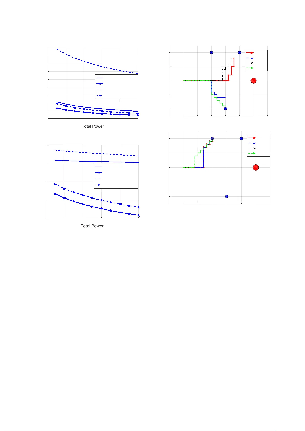
IEEE TRANSA CTIONS ON COMMUNICA TIONS 1 Po wer -Distortion Metrics for P ath Planning o v er Gaussian Sensor Networks Emrah Akyol, Member , IEEE, and Urbashi Mitra, F ellow , IEEE Abstract —Path planning is an important component of au- tonomous mobile sensing systems. This paper studies upper and lower bounds of communication performance over Gaussian sen- sor networks, to drive power-distortion metrics for path planning problems. The Gaussian multiple-access channel is employed as a channel model and two source models are considered. In the first setting, the underlying source is estimated with minimum mean squared error , while in the second, reconstruction of a random spatial field is considered. For both problem settings, the upper and the lower bounds of sensor power-distortion curve are derived. F or both settings, the upper bounds follow from the amplify-and-f orward scheme and the lower bounds admit a unified derivation based on data processing inequality and tensorization property of the maximal correlation measure. Next, closed-form solutions of the optimal power allocation problems are obtained under a weighted sum-power constraint. The gap between the upper and the lower bounds is analyzed f or both weighted sum and individual power constrained settings. Finally , these metrics are used to drive a path planning algorithm and the effects of power-distortion metrics, network parameters, and power optimization on the optimized path selection are analyzed. Index T erms —path planning, underwater communications, Gaussian sensor networks I . I N T RO D U C T I O N Sensor networks can provide monitoring and sensing, for surveillance and localization applications as well as scientific studies, over a wide variety of en vironments such as agri- cultural fields, desert climes, and underwater systems [2]. In many of these applications, the coverage area of interest is so large that inter-sensor communication is not cost-effecti v e or feasible. For example, in underwater en vironmental sensing, the ocean is vast and sensors are unlikely to be densely deployed. In these scenarios, it is energy-ef ficient and cost- effecti v e to employ an autonomous data collecting vehicle (A V) that can travel to all sensors and download the data. In order to communicate with the sensors the A V must be physically close to each sensor , trav eling along a path. The path planning pr oblem in this context is to find the optimal route along which the A V can collect the data from all sensors at maximum quality with minimal resource use (such as E. Akyol (akyol@illinois.edu) is with the Coordinated Science Laboratory , Univ ersity of Illinois at Urbana-Champaign. U. Mitra (ubli@usc.edu) is with the Electrical Engineering Department, Univ ersity of Southern California. This research was funded in part by one or all of these grants: ONR N00014-09-1-0700 AFOSR F A9550-12-1-0215 DO T CA-26-7084-00 NSF CCF-1117896 NSF CNS-1213128 NSF CCF-1410009 NSF CPS-1446901. Part of the material in this paper was presented at the Allerton Conference on Communication, Control and Computing, Urbana, Illinois, Oct. 2014 [1]. ov erall traveling distance, delay , or total energy spent at the sensors for communication) [3]–[10]. In this paper, we consider lossy reconstruction of the data with minimal distortion and with minimal ener gy spent at the sensors. More specifically , we derive and analyze the power - distortion characterization of the fundamental limits of com- munication ov er sensor networks, with the goal of providing meaningful metrics for robotic path planning. In general, an A V may have two different types of objecti ves: to estimate the underlying random source, which is typically modeled as a random process in time (referred as source reconstruction, SR, throughout the paper); or to reconstruct the spatial random field generated by the source (field reconstruction, FR). Consider the motiv ating example in Fig. 1 which in v olves one memoryless source and three static sensors. The objective of the A V is to collect source data from the sensors. Each sensor observes the source ov er a noisy “sensing” channel whose quality depends on the distance between the sensor and the source as follows: if a sensor is closer to the source, it senses the source ov er a less noisy channel. The sensors transmit their observation to A V ov er a multiple-access chan- nel. In the first setting of interest, the objectiv e of the A V is to estimate the source signal (SR). It is then intuitiv ely expected that the A V chooses a path tow ard the sensor(s) which are closest to the source (similar to path (a) in Fig. 1), since they represent the underlying source at maximum fidelity . In the second setting, the objectiv e is to reconstruct the entire spatial random field using the measurements at the sensors. This setting corresponds to a class of en vironmental monitoring applications where physical quantities, such as the temperature, pressure etc. are tracked. In this second case, which we refer as field reconstruction (FR), the objectiv e of the A V simplifies to estimating the sensor measurements, i.e., noisy observ ations of the source, with minimal weighted distortion, where the weights represent the importance of the associated sensor measurement in reconstructing the spatial field. It is intuitively expected that the optimal A V route would be tow ard the sensors whose measurements represent the largest field ( i.e. , the largest weight). In our running example in Fig. 1, the optimal path could look like path (b). In this paper , we formalize these two classes of distortion metrics and analyze the ef fects of them on the optimized path selection. W e study the power -distortion metrics on a Gaussian sensor network model, see e.g., [11]–[19]. In [12], the performance of a simple amplify-and-forward (AF) scheme is studied, in conjunction with optimal po wer assignment over the sensors giv en a sum-po wer budget. For a particular symmetric setting, Gastpar showed that indeed the AF scheme is optimal over all 2 IEEE TRANSA CTIONS ON COMMUNICA TIONS 1 2 3 Source AV (a) (b) Fig. 1: The underwater data gathering example. encoding/decoding methods that allow arbitrarily high delay [20]. Howe ver , it was also sho wn that, in more realistic asymmetric settings, the AF scheme may be suboptimal [21]. In [22], optimal communication strategies were studied for transmitting jointly Gaussian sources o ver a Gaussian MA C. In general, the optimal communication strategies are unknown for both of these settings [23]. W e note that there are other sensor network models beyond the one in this paper, see e.g., [24], and the references therein. V ector settings, associated with the SR metric in our model, were studied in [12] and [19]. Our preliminary results appeared in [1]. The effects of active sensing and adversarial nodes in communications ov er sensor networks were analyzed in [25] and [26], respectively . Information theoretic analysis of the scaling beha vior of such sensor networks was considered in [27]. The contributions of this paper are the follo wing: • Building on [22] and [20], we deri v e the lower and the up- per bounds of the po wer-distortion functions for the two problem settings. The upper bounds are obtained through the AF scheme, while the lo wer bounds follow from the data processing inequality used in conjunction with the tensorization property of the maximal correlation, also known as the W itsenhausen’ s lemma [28]. • For each of these metrics, we derive, in closed-form, strategies for optimal the power allocation ov er sensors subject to a weighted-sum power constraint. Perhaps sur - prisingly , in all cases, the original problem is non-conv ex in the individual po wer allocation variables, ho we ver it can be translated into a conv ex optimization problem that admits a closed-form solution. • W e provide numerical analysis of the dif ferent metrics and uncover cases where the gap between the upper and the lo wer bounds is small (or large), implying the near optimality of the AF scheme (or the need for more sophisticated coding schemes). Our results associated with the SR metric imply that when the sensing and the communication channels are matched- i.e, the sensor with better sensing channel has the better communication channel- the performance loss due to using the AF scheme is low . On the other hand, this loss increases when the sensing and the communication channels are in v ersely matched, i.e., when the sensor with the better sensing channel has the worse communication channel. Howe v er , for the FR metric, the AF scheme performs significantly worse than the lo wer bound. W e also observe that in general, the lower bounds are more sensitive to the choice of parameters than the upper bounds. • Based on the proposed metrics, we implement a simple path planning algorithm. W e analyze, via numerical sim- ulations, the impact of power optimization and metric selection on the rob ustness of the path planning to the sensing/communication channel parameters and the net- work topology . This paper is organized as follo ws: we present the communi- cation model along with the specific metrics in Section II. W e present our results reg arding lo wer and upper bounds of com- munication performance with and without po wer optimization in Section III. W e numerically analyze these metrics and their use in path planning in Section IV . W e present conclusions and discussion in Section V . I I . C O M M U N I C A T I O N M O D E L A. Notation Let E ( · ) and || · || 2 denote the expectation and l 2 norm operators, and R and R + denote the set of real and posi- tiv e real numbers, respectiv ely . In general, lo wercase letters ( e.g . , x ) denote scalars, boldface lowercase ( e.g . , x ) vectors, uppercase ( e.g . , U, X ) matrices and random variables, and boldface uppercase ( e.g . , X ) random vectors. Unless otherwise specified, vectors and random vectors hav e length m , and matrices hav e size m × m . The k th element of vector x is denoted by [ x ] k and the ( i, j ) th element and the k th column of the matrix A are denoted by [ A ] ij and [ A ] k respectiv ely . Let A T denote the transpose of matrix A . A diagonal matrix with diagonal elements a is denoted by diag ( a ) . R X and R X Z denote the auto-cov ariance of X and cross cov ariance of X and Z respecti vely . Gaussian distribution with mean µ and cov ariance matrix R is denoted as N ( µ , R ) . The mutual information between random v ariables X and Y is denoted as I ( X ; Y ) . B. Pr oblem Definition The problem setting is depicted in Fig. 2 where the un- derlying source { S ( i ) } is a sequence of independently and identically distributed (i.i.d.) real v alued Gaussian random variables with zero mean and unit variance, without loss of generality . W e consider a pre-deployed network of M sensors. Sensor m observes a sequence { U m ( i ) } defined as U m ( i ) = β m S ( i ) + W m ( i ) , (1) where { W m ( i ) } is a sequence of i.i.d. Gaussian random vari- ables with zero mean and unit v ariance, independent of { S ( i ) } . Sensor m applies the encoding function g N m : R N → R N to the observation sequence of length N , U m to generate a sequence of channel inputs X m = g N m ( U m ) that satisfies 1 N N X i =1 E { X 2 m ( i ) } ≤ P m (2) where P m is the individual po wer constraint on sensor m . This problem formulation presumes fixed power budget, P m , SUBMITTED P APER 3     SENSOR M SENSOR 1 . . . . . . U 1 U M X M X 1 Y REC. SENSOR 2 X 2 U 2  1  2  M ↵ M ↵ 2 ↵ 1 Z ⇠ N (0 , 1) S ⇠ N (0 , 1) ˆ S, ˆ U 1 ,..., ˆ U M W 1 ⇠ N (0 , 1) W 2 ⇠ N (0 , 1) W M ⇠ N (0 , 1) Fig. 2: The sensor network model for each sensor . Another problem setting we consider in volv es a weighted sum-po wer constraint in the form of 1 N M X m =1 r m N X i =1 E { X 2 m ( i ) } ≤ P T , (3) where the weight vector r = [ r 1 , r 2 . . . r M ] is kno wn. The channel output is Y ( i ) = Z ( i ) + M X m =1 α m X m ( i ) , (4) where { Z ( i ) } is a sequence of i.i.d. Gaussian random variables of zero mean and unit variance, independent of { S ( i ) } and { W m ( i ) } . The recei ver applies a function h N : R N → R N to the receiv ed sequence { Y } to minimize the cost-which is defined explicitly in the next section for each scenario of interest. W ith a slight abuse of notation, we let J ( P ) denote the distortion metric with the power allocation vector P = [ P 1 , P 2 , . . . , P M ] (assigned power to the sensor m is denoted by P m ), and J ( P T ) denote the metric with total power P T with optimized po wer allocation. The sensor network parameters, β , and the communication channel parameters, α , are fixed and known to the sensors and the receiv er; and the block- length N is asymptotically large, i.e., N → ∞ . I I I . D I S T O RT I O N M E T R I C S A. Sour ce r econstruction The source reconstruction (SR) metric, denoted as J S , in v olves estimating the underlying source S with minimum mean squared error (MSE): J S ( P ) , lim N →∞ 1 N N X i =1 E { ( S ( i ) − ˆ S ( i )) 2 } , (5) where ˆ S ( i ) is the estimate of S ( i ) at the receiv er . While the exact characterization of J S ( P ) is in general difficult [23], we state upper and lower bounds of J S ( P ) in the follo wing theorem. Theorem 1. F or any given P , J L S ( P ) ≤ J S ( P ) ≤ J U S ( P ) holds where J U S ( P ) and J L S ( P ) are given in (6) and (7) r espectively . Pr oof: The deri v ation of J U S ( P ) follows directly from the AF communication scheme, where each sensor scales its input U m ( i ) , symbol-by-symbol, to match E { X 2 m ( i ) } to the allowed power P m for each time instant i , i.e. , X m ( i ) = q P m 1+ β 2 m U m ( i ) . W e have J U S ( P ) = E { S 2 } − E { S Y } ( E { Y 2 } ) − 1 E { Y S } (8) where E { S Y } = M X m =1 β m α m s P m 1 + β 2 m , (9) and E { Y 2 } = 1 + M X m =1 β m α m s P m 1 + β 2 m ! 2 + M X m =1 α 2 m P m 1 + β 2 m . (10) Plugging (9) and (10) into (8), we obtain (6). For J L S ( P ) , we follow the steps in [20] to generalize its main result for the symmetric setting to the asymmetric setting considered here. First, we note that from the data processing theorem, we must ha ve I ( U 1 , U 2 , . . . , U M ; ˆ S ) ≤ I ( X 1 , X 2 , . . . , X M ; Y ) (11) The left hand side can be lower bounded as: I ( U 1 , U 2 , . . . , U M ; ˆ S ) ≥ N R ( D ) (12) where R ( D ) is deri ved in the Appendix A. The right hand side can be upper bounded by I ( X 1 , . . . , X M ; Y ) ≤ N X i =1 I ( X 1 ( i ) , . . . , X M ( i ); Y ( i )) (13) ≤ max N X i =1 I ( X 1 ( i ) , . . . , X M ( i ); Y ( i )) (14) = 1 2 N X i =1 log( 1 + α T R X ( i ) α ) (15) 4 IEEE TRANSA CTIONS ON COMMUNICA TIONS J U S ( P ) = 1 + M P m =1 α 2 m P m 1+ β 2 m 1 +  M P m =1 β m α m q P m 1+ β 2 m  2 + M P m =1 α 2 m P m 1+ β 2 m , (6) J L S ( P ) = 1 1 + M P m =1 β 2 m      1 + M P m =1 β 2 m 1 + M P m =1 α 2 m P m 1 + β 2 m +  M P m =1 β m α m q P m 1 + β 2 m  2      . (7) where R X ( i ) is defined as { R X ( i ) } p,r , E { X p ( i ) X r ( i ) } ∀ p, r ∈ [1 : M ] . (16) Note that (13) follo ws from the memoryless property of the channel and the maximum in (14) is over the joint density of X 1 ( i ) , . . . , X M + K ( i ) , giv en the structural constraints on R X ( i ) due to the power constraints. It is well kno wn that the maximum is achie ved by the jointly Gaussian density for a giv en co v ariance, yielding (15). Since the logarithm is a mono- tonically increasing function, the optimal encoding functions g N m ( · ) , m ∈ [1 : M ] equivalently maximize P p,r E { X p ( i ) X r ( i ) } for all i . Note that X m = g N m ( U m ) (17) and hence the g N m ( · ) , m ∈ [1 : M ] that maximize P p,r E { X p ( i ) X r ( i ) } can be found by inv oking Witsenhausen’ s lemma (gi ven in Appendix C) as X m ( i ) = γ N U m where γ N = s P m 1 + β 2 m , . . . , s P m 1 + β 2 m ! . (18) Plugging (18) in (12), we have R = 1 2 log   1 + M X m =1 α 2 m P m 1 + β 2 m + M X m =1 β m α m s P m 1 + β 2 m ! 2   (19) Plugging the expression for R ( D ) (deri ved in the Appendix A) in (75), we obtain (7). Remark 1. It is of interest to see whether the mutual in- formation or source SNR based metrics (see e.g., [29], [30]) ar e of use here . Noting that S and ˆ S used in the derivation of both lower and upper bounds are jointly Gaussian, it is straightforwar d to show that I ( S ; ˆ S ) = − 1 2 log J S ( P ) . Hence, minimizing J S ( P ) and maximizing I ( S ; ˆ S ) ar e effectively identical for path selection purposes. The same conclusion also holds for the field r econstruction metric (defined in the next section) by similar arguments. Also note that the sour ce SNR is exactly 1 /J S ( P ) and hence, maximizing sour ce SNR is equivalent to minimizing J S ( P ) . Next, we discuss the optimal po wer allocation among sensors and derive the optimal trade-off between distortion metrics and the weighted sum of transmit po wer . P articularly , we study the follo wing optimization problem: minimize P 1 ,P 2 ,...,P M J S ( P 1 , P 2 , . . . , P M ) subject to M X m =1 r m P m ≤ P T where r = [ r 1 , r 2 , . . . , r M ] and P T are giv en optimization parameters. The following theorem states the P T versus J S relationship when the po wer allocation is optimized. Theorem 2. F or any given P T and a weight vector r = [ r 1 , r 2 . . . r M ] , J L S ( P T ) ≤ J S ( P T ) ≤ J U S ( P T ) holds wher e J U S ( P T ) = 1 + P T M X m =1 α 2 m β 2 m r m + r m β 2 m + P T α 2 m ! − 1 (20) J L S ( P T ) = 1 1 + M P m =1 β 2 m     1 + M P m =1 β 2 m 1 + P T λ     (21) and λ satisfies M X m =1 α 2 m β 2 m r m + r m β 2 m − λα 2 m = 1 λ . (22) Pr oof: J U S ( P T ) : The proof follows from similar steps of the proof of Theorem 4 of [12] with appropriate changes due to the weight v ector r , and is omitted. J L S ( P T ) : Minimization of J L S ( P ) in P is equiv alent to minimizing D = − M X m =1 β m α m s P m 1 + β 2 m ! 2 − M X m =1 α 2 m P m 1 + β 2 m (23) subject to M P m =1 r m P m ≤ P T ov er P m ≥ 0 for all m . This objectiv e function is not con v ex 1 in the variables P m . W e first impose a slackness v ariable t = M X m =1 α m β m s P m 1 + β 2 m . (24) and analyze the dual problem: minimize M X m =1 r m P m , (25) 1 This can easily be shown by checking the positive definiteness Hessian of the objectiv e function. SUBMITTED P APER 5 subject to − D − M X m =1 α 2 m P m 1 + β 2 m ≤ t 2 , (26) and (24). This problem is conv e x in the variables P m and t , and can be con verted into unconstrained optimization problem: minimize J = M X m =1 r m P m + λ 1 − D − M X m =1 α 2 m P m 1 + β 2 m − t 2 ! + λ 2 t − M X m =1 α m β m s P m 1 + β 2 m ! , (27) where λ 1 ∈ R + and λ 2 ∈ R . Next, we note that Karush- Kuhn-T ucker (KKT) optimality conditions are sufficient for this problem (no duality gap) since the objectiv e function is con v ex in the v ariables P m and t [31]. W e determine the KKT conditions: ∂ J ∂ P m = r m − λ 1 α 2 m 1 + β 2 m − λ 2 α m β m 2 p P m (1 + β 2 m ) = 0 , (28) ∂ J ∂ t = − 2 λ 1 t + λ 2 = 0 , (29) − D − M X m =1 α 2 m P m 1 + β 2 m = t 2 , (30) and we ha ve (24). From (28), we obtain P m in terms of λ 1 and λ 2 as P m = λ 2 2 4 α 2 m β 2 m (1 + β 2 m ) ( r m + r m β 2 m − λ 1 α 2 m ) 2 . (31) Plugging (31) into (24), we have t = λ 2 2 M X m =1 α 2 m β 2 m r m + r m β 2 m − λ 1 α 2 m . (32) Re-writing (30) using (29) and (32), we hav e λ 2 2 4 λ 1 M X m =1 α 2 m β 2 m r m + r m β 2 m − λ 1 α 2 m = − D − λ 2 2 4 M X m =1 α 4 m β 2 m ( r m + r m β 2 m − λ 1 α 2 m ) 2 (33) which simplifies to − D = λ 2 2 4 λ 1 M X m =1 r m (1 + β 2 m ) α 2 m β 2 m ( r m + r m β 2 m − λ 1 α 2 m ) 2 (34) = 1 λ 1 M X m =1 r m P m = P T λ 1 . (35) Expressing (32) using (29), we obtain (22). Using (35), we obtain (21). Remark 2. The coefficient λ is a Lagrange parameter in a con ve x optimization pr oblem, as demonstrated in the proof above; hence, the solution of (22) exists and it is unique [31]. It can be found numerically by a bisection sear c h. In practice, the computational complexity of determining λ is r elatively low , since it is computed only once for each network setting, i.e., it does not depend on P T . B. F ield Reconstruction In the field reconstruction (FR) setting, the objectiv e of the receiv er is to estimate the entire random field which is cov ered by the sensors. W e assume that at any point is represented by the closest sensor , or alternatively a linear interpolation of the closest k sensors readings. Hence, we define the FR metric as J F ( P ) , lim N →∞ 1 N N X i =1 M X m =1 γ m E { ( U m ( i ) − ˆ U m ( i )) 2 } (36) where the γ m are determined by k and network parameters ( i.e. , sensor locations). Before stating the results, we define the cov ariance matrix of sensor inputs U , i.e., R U , E { U U T } which can explicitly be expressed as a function of β R U =      1 + β 2 1 β 1 β 2 . . . β 1 β M β 1 β 2 1 + β 2 2 . . . β 2 β M . . . . . . . . . β 1 β M . . . 1 + β 2 M      . (37) R U admits an eigen-decomposition R U = Q T U Λ Q U where Q U is unitary and Λ is a diagonal matrix with elements 1 , . . . , 1 , 1 + P m β 2 m . The following transformed weight vector is used in the subsequent results: γ 0 k , [ Q T U diag( γ ) Q U ] kk . (38) Again, the complete characterization of J F ( P ) is difficult in general [23], and similar to the SR case, we state upper and lower bounds in the follo wing theorem. In the deriv ation of J U F ( P ) , we assume a high power (low distortion) regime, in order to simplify e xposition. Theorem 3. F or a given P , J L F ( P ) ≤ J F ( P ) ≤ J U F ( P ) holds, wher e J U F ( P ) and J L F ( P ) ar e given in (39) and (40) r espectively . wher e A = M P m =1 β m α m q P m 1+ β 2 m . Pr oof: The deriv ation of J U F ( P ) follows from the AF scheme, where for each m , we have J m = E { U 2 m } − E { U m Y } ( E { Y 2 } ) − 1 E { Y U m } (41) Noting that E { U m Y } = α m s P m 1 + β 2 m + β m M X m =1 β m α m s P m 1 + β 2 m , (42) and using the expression for ( E { Y 2 } ) − 1 giv en in (10), we hav e: J m = 1 + β 2 m −  α m q P m 1+ β 2 m + β m M P m =1 β m α m q P m 1+ β 2 m  2 1 +  M P m =1 β m α m q P m 1+ β 2 m  2 + M P m =1 α 2 m P m 1+ β 2 m . (43) Noting that J U F ( P ) = M P m =1 γ m J m , we obtain (39). T o derive J L F ( P ) , we follo w the steps (11)-(19) verbatim , with the difference that we use vector R ( D ) (derived in Appendix B) instead of R ( D ) associated with remote compression. Combining (19) with (84), we obtain (40). 6 IEEE TRANSA CTIONS ON COMMUNICA TIONS J U F ( P ) = − M P m =1 γ m α 2 m P m 1 + β 2 m + A 2  M P m =1 γ m β 2 m  + 2 A  M P m =1 γ m β m α m q P m 1 + β 2 m  1 + A 2 + M P m =1 α 2 m P m 1+ β 2 m + M X m =1 γ m (1 + β 2 m ) (39) J L F ( P ) = M (1 + M X m =1 β 2 m ) M Y m =1 γ 0 m ! 1 M 1 + M X m =1 α 2 m P m 1 + β 2 m + A 2 ! − 1 M (40) Remark 3. As a side note, by (76), we note that γ majorizes γ 0 (see [32, 2.B.3]) which implies that M Q m =1 γ 0 m ≥ M Q m =1 γ m . A looser bound (independent of γ 0 ) can be obtained by replacing γ 0 with γ . Next, we optimize power allocation ov er the sensors. For notational con venience, here we assume 2 γ m = 1 for all m . The following theorem states the upper and lower bounds of the FR metric with power optimization. Theorem 4. F or any given P T and r = [ r 1 , r 2 . . . r M ] , J L F ( P T ) ≤ J F ( P T ) ≤ J U F ( P T ) holds wher e J U F ( P T ) = M + M X m =1 β 2 m + P T λ 1 − P T , (44) J L F ( P T ) = M 1 + M X m =1 β 2 m ! λ 2 P T ! 1 M , (45) and λ 1 and λ 2 satisfy  − 1 −  1 − P T λ 1  1 + M X m =1 β 2 m ! × M X m =1 α 2 m β 2 m r m + r m β 2 m + λ 1 α 2 m = 1 λ 1 , (46) M X m =1 α 2 m β 2 m r m + r m β 2 m − λ 2 α 2 m = 1 λ 2 . (47) Pr oof: Plugging γ m = 1 for all m in (39), we have (48). Minimization of J U F ( P ) in P is equi v alent to minimizing D = − M P m =1 α 2 m P m 1+ β 2 m +  2 + M P m =1 β 2 m   M P m =1 β m α m q P m 1+ β 2 m  2 1 +  M P m =1 β m α m q P m 1+ β 2 m  2 + M P m =1 α 2 m P m 1+ β 2 m (49) subject to M X m =1 r m P m ≤ P T (50) for P m ≥ 0 for all m . This objectiv e function is not con v ex in P m . Follo wing similar steps to those in the proof of Theorem 2 Note that this assumption does not introduce any loss of generality , since γ can be incorporated into the power scaling coefficients β in the problem definition. 2, we first con v ert the problem into a con ve x form introducing a slack v ariable t = M X m =1 α m β m s P m 1 + β 2 m , (51) and express the optimizing problem as to minimize M P m =1 r m P m subject to D 1 + D + M X m =1 α 2 m P m 1 + β 2 m ≤ δ t 2 , (52) and (51) where δ , − 1 − 1 + M P m =1 β 2 m 1 + D . (53) This problem is con vex in the v ariables P m and t , hence can be con v erted into an unconstrained optimization problem where we minimize J = M X m =1 r m P m + λ 1 D 1 + D + M X m =1 α 2 m P m 1 + β 2 m − δ t 2 ! (54) + λ 2 t − M X m =1 α m β m s P m 1 + β 2 m ! , (55) where λ 1 ∈ R + and λ 2 ∈ R . Applying the KKT conditions, we hav e ∂ J ∂ P m = r m + λ 1 α 2 m 1 + β 2 m − λ 2 α m β m 2 p P m (1 + β 2 m ) = 0 , (56) ∂ J ∂ t = − 2 λ 1 δ t + λ 2 = 0 , (57) ∂ J ∂ λ 1 = D 1 + D + M X m =1 α 2 m P m 1 + β 2 m − δ t 2 = 0 . (58) From (56), we obtain P m in terms of λ 1 and λ 2 as P m = λ 2 2 4 α 2 m β 2 m (1 + β 2 m ) ( r m + r m β 2 m + λ 1 α 2 m ) 2 . (59) Plugging (59) in (51), we have t = λ 2 2 M X m =1 α 2 m β 2 m r m + r m β 2 m + λ 1 α 2 m . (60) Re-writing (58) using (57) and (60), we hav e (61) which SUBMITTED P APER 7 J U F ( P ) = M + M X m =1 β 2 m − M P m =1 α 2 m P m 1+ β 2 m +  2 + M P m =1 β 2 m   M P m =1 β m α m q P m 1+ β 2 m  2 1 +  M P m =1 β m α m q P m 1+ β 2 m  2 + M P m =1 α 2 m P m 1+ β 2 m (48) λ 2 2 4 λ 1 M X m =1 α 2 m β 2 m r m + r m β 2 m + λ 1 α 2 m = D 1 + D + λ 2 2 4 M X m =1 α 4 m β 2 m ( r m + r m β 2 m + λ 1 α 2 m ) 2 (61) simplifies to λ 1 D 1 + D = λ 2 2 4 M X m =1 r m (1 + β 2 m ) α 2 m β 2 m ( r m + r m β 2 m + λ 1 α 2 m ) 2 (62) = M X m =1 r m P m = P T . (63) Plugging (63) in (48), we obtain J U F ( P T ) . Plugging (53), (57), and (63) in (60), we obtain (46). J L F ( P T ) : Minimization of J L F ( P ) in P is equiv alent to minimizing D = − M X m =1 β m α m s P m 1 + β 2 m ! 2 − M X m =1 α 2 m P m 1 + β 2 m , (64) subject to M P m =1 r m P m ≤ P T and P m ≥ 0 for all m . This problem is solved in the proof of Theorem 2, hence we follow the same steps as in (24)-(35) and obtain J L F ( P T ) . Remark 4. Similar to the SR setting (see Remark 2), λ 1 and λ 2 in (47) and (46) are in fact Lagrange parameter s in a con ve x optimization pr oblem as shown in the pr oof above, hence they exist and they are unique [31]. Unlike (22), the computation of λ 1 in (46) depends on P T in addition to α and β . However , for a given P T , the computation employs similar steps. Remark 5. The optimal power allocation strate gies in both SR and FR settings can be implemented by each sensor in a distributed manner: the central ag ent (e.g ., the A V) computes the optimal values of λ 1 and λ 2 (or λ in SR setting), and br oadcasts this information to all sensors. Each sensor then computes its own power allocation based on local parameter s α m and β m and the br oadcasted global parameters λ 1 and λ 2 (or λ ). I V . N U M E R I C A L R E S U LT S W e first analyze different metrics, particularly the gap between upper and lower bounds and the impact of power optimization. Next, we focus on the problem of path planning in conjunction with these metrics. A. Metrics In our experiments, we select α and β randomly , uniformly from the interval [0 , 1] . T o analyze the impact of sensing and communication channel ordering on the metrics, we look at Power 4 6 8 10 12 14 MSE 0.4 0.45 0.5 0.55 0.6 0.65 0.7 J U S (matched) J L S (matched) J U S (inversely matched) J L S (inversely matched) (a) Comparison of MSE bounds for matched and mismatched channels for source reconstruction. Power 4 6 8 10 12 14 Weighted MSE 2.5 3 3.5 4 4.5 5 J U F (matched) J L F (matched) J U F (inversely matched) J L F (inversely matched) (b) Comparison of MSE bounds for matched and mismatched channels for field reconstruction. Fig. 3: MSE bounds for uniform power allocation. two extreme cases: i) ordered channels, i.e. , the better sensing channel (larger β ) is matched to better communication channel (larger α ), ii) rev erse ordered, i.e. , larger β is matched to smaller α . For the FR metric, we set γ m = 1 for all m . T o obtain statistically meaningful results, we av erage the results ov er 10000 runs of this experiment. W e set the number of sensors 5, i.e., M = 5 . In Fig. 3, we plot the comparati ve results with individual power constraints. All sensors are assumed to have identical power , P m = P for all m . As can be seen numerically , when the sensing and the communication channels are matched, i.e. , the sensor with the better sensing channel sees a better 8 IEEE TRANSA CTIONS ON COMMUNICA TIONS Total Power 20 30 40 50 60 70 MSE 0.4 0.42 0.44 0.46 0.48 0.5 0.52 0.54 0.56 0.58 J U S (matched) J L S (matched) J U S (inversely matched) J L S (inversely matched) (a) Comparison of MSE bounds for matched and mismatched channels for source reconstruction. Total Power 20 30 40 50 60 70 Weighted MSE 2.5 3 3.5 4 4.5 J U F (matched) J L F (matched) J U F (inversely matched) J L F (inversely matched) (b) Comparison of MSE bounds for matched and mismatched channels for field reconstruction. Fig. 4: MSE bounds for optimized power allocation. communication channel, the gap between upper and lower bounds is small, and as they get mismatched, this gap widens. An important observ ation is that in the matched order case, upper and lower bounds perform very close for both settings, particularly for the SR setting. In Fig. 4, we plot the comparati ve results with a total po wer constraint, with r m = 1 for all m . B. P ath Planning Results T o obtain the optimal paths giv en these metrics, we use a simple search algorithm based on determining the step (in four directions) at each point in a greedy manner , i.e., the A V at location ( i, j ) moves to ( i ± 1 , j ) or ( i, j ± 1) or stays at ( i, j ) depending on the cost at these locations. More sophisticated search algorithms can be found in the robotics literature (see e.g ., [7] and the references therein). W e note that the optimal path will depend on the specific search algorithm used. Our objectiv e here is to demonstrate the use of the proposed metrics in path planning, and their implications on the chosen path, i.e., the type of distortion metric chosen and network parameters affect the optimal path significantly . Our numerical -1.5 -1 -0.5 0 0.5 1 1.5 2 -1 -0.5 0 0.5 1 Sensor 1 Sensor 2 Sensor 3 Source J U S ( P ) J U F ( P ) J U S ( P T ) J U F ( P T ) (a) Paths driven by upper bounds -1.5 -1 -0.5 0 0.5 1 1.5 2 -1 -0.5 0 0.5 1 Sensor 1 Sensor 2 Sensor 3 Source J L S ( P ) J L F ( P ) J L S ( P T ) J L F ( P T ) (b) Paths driven by lower bounds Fig. 5: Paths chosen in network topology-1 examples demonstrate this conclusion via numerical examples generated using this simple search algorithm. W e consider two network topologies, both of which inv olv e three sensors and one source. The sensing parameters β are chosen as in v ersely proportional with the squared distances between the sensor and the source, i.e., for source and m th sensor locations x s and x m , we ha ve β m = b × || x s − x m || − 2 2 for some b ∈ R + . The channel parameters, α , are determined similarly: giv en the A V location x a , we hav e α m = a × || x a − x m || − 2 2 , for a giv en a ∈ R + . The path step size is set to 0 . 01 and paths are of length 30 steps, and the weight vector r = [1 , 1 , 1] . The A V is set to point [ − 1 , 0] on a 3 × 3 . 5 grid and source location is set to [1 . 5 , 0] . W e provide two examples that demonstrate dif ferent aspects of path selection and metrics. W e first consider a network topology similar to the motiv at- ing example in Fig. 1, where an A V gathers data from three deployed sensors. W e choose a = b = 10 , and P m = 10 for each sensor, hence P T = 30 , and γ = [1 , 1 , 4] to capture the effect of non-symmetry in the network topology . W e plot the paths chosen by upper bounds metrics, in Fig. 5(a) and ones with the lo wer bounds, in Fig. 5(b) Here, the upper bounds (obtained via the AF scheme) of the SR metric yields a path tow ards the sensors closest to the source, as sho wn in Fig. 5(a). Power optimization makes this path only more skewed toward the closest sensor (sensor -1), which is theoretically expected since sensor 1 senses the source with minimum distortion, and SUBMITTED P APER 9 hence more po wer is allo wed for sensor-1 in the optimized power allocation method. The upper bound of the FR metric (achiev ed via the AF scheme) results in a path tow ards sensor- 3, which is due to fact that sensor-3 represents a larger area than other sensors and, hence the asymmetry in γ . Therefore, the numerical path selection results demonstrated in Fig. 5(a) confirm our intuition in the e xample in Fig. 1. Howe ver , for the lower bounds, all four metrics yield the same path tow ards to the closest sensor to the A V (sensor-2). The results in this example indicate a very inter esting conclusion on the importance of the metric selection, since the optimal paths in this e xample str ongly depend on the metric chosen. Next, we change the network topology to a semi-symmetric version where two of the sensors (sensors 1 and 3) are equally distant from the source. In this example, we analyze the impact of channel parameters on the metrics and ev entually path selection. Since the settings is relatively more symmetric (as opposed to previous setting), we set γ = [1 , 1 , 1] and r = [1 , 1 , 1] . W e plot the paths found for parameter values a = 10 , b = 1 , and P m = 100 for all m in Fig. 6. Note that this example presents an interesting case for path selection, since paths chosen by different metrics vary widely . First, let us explain why J U S ( P ) and J U F ( P ) yield these paths. An obvious question is the following: why do these paths tend to mov e away from all the sensors and source in the beginning of the path? The answer lies in the network parameters and topology . This example in volv es a very small sensing parameter , ( b ), compared to communication parameters, ( a and P ), which implies that the sensor with the worst sensing channel can ev en amplify ov erall noise at the A V , i.e., sensor-2 output interferes with the source S , in SR case, or with other sensor observations U m in the FR case. Note that A V can only change its communication channel quality while the sensing channel is fixed in the problem setting. This indicates that the A V can only mitigate the effect of these ”bad sensors” (here sensor-2) by moving a way from them. This is exactly what we observe in Fig. 6(a) for the paths generated by J U S ( P ) and J U F ( P ) . Note that due to symmetry overall costs (when measured by the same metric) of both paths are identical (in Fig. 6(a), these two paths with identical costs are assigned to J U S ( P ) and J U F ( P ) randomly). When po wer is optimized, sensor-2 is not allo wed to decrease the communication channel SNR at the A V ( P 2  10 ), hence the paths by J U S ( P T ) and J U F ( P T ) are towards to the middle of all sensors due to symmetry . Note that all lo wer bounds yields the same path for this example. Next, in the same network topology , we increase the sensing parameter b and decrease the communication parameters, a and P , specifically , we set a = 1 , b = 10 , P m = 10 for all m , and hence P T = 30 , and keep other parameters the same as the previous setting ( r = [1 , 1 , 1] , γ = [1 , 1 , 1] ). For these settings, as Fig. 7 demonstrates, all metrics yield a path toward the closest sensor to A V , which is sensor-2 in this setting. This is theoretically expected since the bottleneck for the performance here is the communication over MA C, as opposed to the sensing channel (which was the case in the previous setting in Fig. 6) due to channel parameters. -1.5 -1 -0.5 0 0.5 1 1.5 2 -1 -0.5 0 0.5 1 Sensor 1 Sensor 2 Sensor 3 Source J U S ( P ) J U F ( P ) J U S ( P T ) J U F ( P T ) (a) Paths driven by upper bounds -1.5 -1 -0.5 0 0.5 1 1.5 2 -1 -0.5 0 0.5 1 Sensor 1 Sensor 2 Sensor 3 Source J L S ( P ) J L F ( P ) J L S ( P T ) J L F ( P T ) (b) Paths driven by lower bounds Fig. 6: Paths chosen in network topology-2, small sensing parameters V . C O N C L U S I O N S In this paper , we hav e analyzed bounds of communication performance over Gaussian sensor networks for path plan- ning problems. W e have considered two main metrics: i) the underlying source is estimated, and ii) the spatial field is reconstructed. W e have provided a unified proof for the upper and lower bounds of the fundamental limits of communication with these metrics, for fixed and optimized power allocations. Finally , the effect of metric selection, network topology and channel parameters on the selected path is analyzed. Our results show that depending on the network, metric selection and power optimization may significantly impact the optimal path in data gathering. Simulation results suggest that the metrics associated with the lo wer bounds seem to be more sensitiv e to channel parameters and network topology than those of the outer bounds. This paper is concerned static sensors and a mobile data gathering device, and a single scalar source and scalar chan- nels. Our future w ork includes extension to dynamic and multi- source and multi-dimensional settings, and on the optimal resource (power) allocation in time over a fixed path period, and its impact on path selection. Analysis of the settings where sensing is performed in a mobile platform (see e.g., [33]), or partially known or timely varying network statistics are left 10 IEEE TRANSA CTIONS ON COMMUNICA TIONS -1.5 -1 -0.5 0 0.5 1 1.5 2 -1 -0.5 0 0.5 1 Sensor 1 Sensor 2 Sensor 3 Source J U S ( P ) J U F ( P ) J U S ( P T ) J U F ( P T ) (a) Paths driven by upper bounds -1.5 -1 -0.5 0 0.5 1 1.5 2 -1 -0.5 0 0.5 1 Sensor 1 Sensor 2 Sensor 3 Source J L S ( P ) J L F ( P ) J L S ( P T ) J L F ( P T ) (b) Paths driven by lower bounds Fig. 7: Paths chosen in network topology-2, small communi- cation parameters as future work. W e finally note that this paper highlights the need for further information-theoretic analysis of fundamental bounds for sensor netw orks. One research direction is to utilize structured codes [34] in such netw orked source-channel coding problems. A P P E N D I X A G AU S S I A N R E M OT E C O M P R E S S I O N P RO B L E M In this problem, an underlying Gaussian source S ∼ N (0 , 1) is observed under additive noise W ∼ N ( 0 , R W ) as U = S + W . These noisy observations, i.e. , U , must be encoded in such a way that the decoder produces a good approximation to the original underlying source. This problem was proposed in [35] and solved in [36] (see also [37]). A lo wer bound for this function for the non-Gaussian sources within the symmetric setting where all U ’ s hav e identical statistics was presented in [38]. Here, we simply extend the results in [36] to our asymmetric setting, noting D = E { ( S − ˆ S ) 2 } , (65) R = min I ( U ; ˆ S ) , (66) where U = β S + W , W ∼ N ( 0 , R W ) , and R W is an M × M identity matrix. The minimization in (66) is over all conditional densities p ( ˆ s | u ) that satisfy (65). The MSE distortion can be written as sum of two terms D = E { ( S − T + T − ˆ S ) 2 } , (67) = E { ( S − T ) 2 } + E { ( T − ˆ S ) 2 } , (68) where T , E { S | U } . Note that (68) holds since E { ( S − T )( ˆ S − T ) } = 0 , (69) as the estimation error , S − T , is orthogonal to any function 3 of the observ ation, U . The estimation distortion D est , E { ( S − T ) 2 } (70) is constant with respect to p ( ˆ s | u ) . Hence, the minimization is over the densities that satisfy a distortion constraint of the form E { ( T − ˆ S ) 2 } ≤ D rd and R = min I ( U ; ˆ S ) . Hence, we write (68) as D = D rd + D est . (71) Note that due to their Gaussianity , T is a sufficient statistic of U for S , i.e. , S − T − U forms a Markov chain in that order and T ∼ N (0 , σ 2 T ) . Hence, R = min I ( U ; ˆ S ) = min I ( T ; ˆ S ) where minimization is ov er p ( ˆ s | t ) that satisfy E { ( T − ˆ S ) 2 } ≤ D rd , where all v ariables are Gaussian. This is the classical Gaussian rate-distortion problem, and hence: D rd ( R ) = σ 2 T 2 − 2 R . (72) Note that T = R S U R − 1 U U , where R S U , E { S U T } and R U is gi ven in (37). Note that R U is structured, and can easily be manipulated. W e compute σ 2 T as σ 2 T = R S U R − 1 U R T S U = M P m =1 β 2 m 1 + M P m =1 β 2 m , (73) and using standard linear estimation principles, we obtain D est = 1 1 + M P m =1 β 2 m . (74) Plugging (74) in (72) and using (71) yields D =     1 1 + M P m =1 β 2 m + M P m =1 β 2 m 1 + M P m =1 β 2 m 2 − 2 R     . (75) A P P E N D I X B G AU S S I A N V E C TO R S O U R C E C O D I N G The problem of interest to find D ( R ) that minimize D = M P m =1 γ m E { ( U m − ˆ U m ) 2 } , over R m ≥ 0 subject to R = M P m =1 R m . This is a variant of a standard problem of encoding multiple independent Gaussian variables [39]. Note that R U giv en in ( 37 ) accepts the eigen-decomposition 3 Note that ˆ S is also a deterministic function of U , since the optimal reconstruction can always be achiev ed by deterministic codes. SUBMITTED P APER 11 R U = Q T U Λ Q U , where Λ is a diagonal matrix with entries 1 , 1 , . . . , 1 , 1 + M P m =1 β 2 m and Q U is a unitary matrix. Hence, the problem can be conv erted (by linear transformation) to that of encoding independent Gaussian scalars with v ariances 1 , 1 , . . . , 1 + M P m =1 β 2 m , i.e. , we minimize D = M P m =1 γ 0 m D m subject to R = M P m =1 R m , where γ 0 k , [ Q T U diag( γ ) Q U ] kk (76) and R m =  1 2 log  Λ m D m  + . Equi v alently , we minimize J = M X m =1 1 2 log  Λ m D m  + λ M X m =1 γ 0 m D m (77) ov er the set of D m that satisfy D m ≤ Λ m (hence, R m ≥ 0 , ∀ m ). Applying the KKT conditions, we have ∂ J ∂ D m = − 1 2 1 D m + λγ 0 m = 0 , (78) or D m = 1 2 λγ 0 m , θ /γ 0 m . (79) Hence, we ha ve R = 1 2 M X m =1 log  Λ m D m  , (80) where D m = min { θ /γ 0 m , Λ m } , (81) and θ is chosen so that D = M P m =1 γ 0 m D m , for diag ( γ 0 ) = Q T U diag( γ ) Q U . The water-filling nature of the solution (see (81)) pre vents the achie vement of closed-form solutions for the power -distortion curve. T o provide insight, we assume the “high rate” (lo w distortion) regime, where each component is effecti v e, i.e. , θ ≤ min m { Λ m γ 0 m } . W ith this assumption, we hav e D m = θ /γ 0 m , and hence θ = D/ M . (82) Plugging (82) in (80), we have R = 1 2 M X m =1 log (Λ m γ 0 m ) − M 2 log  D M  , (83) and noting that M P m =1 log (Λ m γ 0 m ) = log  M Q m =1 Λ m γ 0 m  = log  (1 + M P m =1 β 2 m ) M Q m =1 γ 0 m  , we ha ve D = M (1 + M X m =1 β 2 m ) M Y m =1 γ 0 m ! 1 M exp  − 2 M R  . (84) A P P E N D I X C W I T S E N H AU S E N ’ S L E M M A Lemma 1 (from [28]) . Consider two sequences of i.i.d. random variables X ( i ) and Y ( i ) , gener ated fr om a joint density P X,Y , and two arbitrary functions f , g : R → R satisfying E { f ( X ) } = E { g ( Y ) } = 0 , E { f 2 ( X ) } = E { g 2 ( Y ) } = 1 . (85) F or any functions f N , g N : R N → R satisfying E { f N ( X ) } = E { g N ( Y ) } = 0 , E { f 2 N ( X ) } = E { g 2 N ( Y ) } = 1 , (86) for length N vectors X and Y , we have sup f N ,g N E { f N ( X ) g N ( Y ) } ≤ sup f ,g E { f ( X ) g ( Y ) } . (87) Mor eover , the supremum abo ve is attained by linear mappings, if P X,Y is Gaussian density . R E F E R E N C E S [1] E. Akyol and U. Mitra, “On source-channel coding over Gaussian sensor networks for path planning, ” in 2014 52nd Annual Allerton Conference on Communication, Control, and Computing . IEEE, 2014, pp. 1140– 1147. [2] I. F . Akyildiz, W . Su, Y . Sankarasubramaniam, and E. Cayirci, “ A surve y on sensor networks, ” IEEE Communications Magazine , vol. 40, no. 8, pp. 102–114, 2002. [3] R.C. Shah, S. Roy , S. Jain, and W . Brunette, “Data mules: modeling a three-tier architecture for sparse sensor networks, ” in Pr oceedings of the First IEEE International W orkshop on Sensor Network Protocols and Applications , May 2003, pp. 30–41. [4] I. V asilescu, K. Kotay , D. Rus, L. Ov ers, P . Sikka, M. Dunbabin, P . Chen, and P . Corke, “Krill: an exploration in underwater sensor networks, ” in Embedded Networked Sensors, 2005. EmNetS-II. The Second IEEE W orkshop on , May 2005, pp. 151–152. [5] O. T ekdas, V . Isler, J. H. Lim, and A. T erzis, “Using mobile robots to harvest data from sensor fields, ” IEEE W ir eless Communications , vol. 16, no. 1, pp. 22, 2009. [6] R. Sugihara and R. Gupta, “Path planning of data mules in sensor networks, ” A CM T ransactions on Sensor Networks , vol. 8, no. 1, pp. 1, 2011. [7] G. Hollinger, S. Choudhary , P . Qarabaqi, C. Murphy , U. Mitra, G. Sukhatme, M. Stojanovic, H. Singh, and F . Hover , “Underwater data collection using robotic sensor networks, ” IEEE Journal on Selected Ar eas in Communications , vol. 30, no. 5, pp. 899–911, 2012. [8] L. He, J. Pan, and J. Xu, “ A progressiv e approach to reducing data collection latency in wireless sensor networks with mobile elements, ” IEEE T ransactions on Mobile Computing , vol. 12, no. 7, pp. 1308–1320, 2013. [9] R. Xu, H. Dai, Z. Jia, M. Qiu, and B. W ang, “ A piecewise geometry method for optimizing the motion planning of data mule in tele-health wireless sensor networks, ” W ireless Networks , vol. 20, no. 7, pp. 1839– 1858, 2014. [10] I. Akyildiz, D. Pompili, and T . Melodia, “Underwater acoustic sensor networks: research challenges, ” Ad hoc networks , vol. 3, no. 3, pp. 257–279, 2005. [11] M. Gastpar and M. V etterli, “Power , spatio-temporal bandwidth, and distortion in large sensor networks, ” IEEE Journal on Selected Ar eas in Communications , vol. 23, no. 4, pp. 745–754, April 2005. [12] J. Xiao, S. Cui, Z. Luo, and A. Goldsmith, “Linear coherent decentral- ized estimation, ” IEEE T ransactions on Signal Pr ocessing , vol. 56, no. 2, pp. 757–770, 2008. [13] J. Li and G. AlRegib, “Distributed estimation in energy-constrained wireless sensor networks, ” IEEE Tr ansactions on Signal Pr ocessing , vol. 57, no. 10, pp. 3746–3758, Oct 2009. [14] A. Ribeiro and G.B. Giannakis, “Bandwidth-constrained distributed estimation for wireless sensor networks-part i: Gaussian case, ” IEEE T r ansactions on Signal Pr ocessing , v ol. 54, no. 3, pp. 1131–1143, March 2006. 12 IEEE TRANSA CTIONS ON COMMUNICA TIONS [15] J. Jin, A. Ribeiro, Luo Z.Q., and G.B. Giannakis, “Distributed compression-estimation using wireless sensor networks, ” IEEE Signal Pr ocessing Magazine , vol. 23, no. 4, pp. 27–41, July 2006. [16] I. Bahceci and A.K. Khandani, “Linear estimation of correlated data in wireless sensor networks with optimum power allocation and analog modulation, ” IEEE T ransactions on Communications , vol. 56, no. 7, pp. 1146–1156, July 2008. [17] F . Jiang, J. Chen, and A.L. Swindlehurst, “Optimal power allocation for parameter tracking in a distrib uted amplify-and-forw ard sensor network, ” IEEE Tr ansactions on Signal Processing , vol. 62, no. 9, pp. 2200–2211, May 2014. [18] H. Behroozi and M.R. Soleymani, “On the optimal power-distortion tradeoff in asymmetric Gaussian sensor network, ” IEEE T ransactions on Communications , vol. 57, no. 6, pp. 1612–1617, June 2009. [19] A. Behbahani, A. Eltawil, and H. Jafarkhani, “Linear decentralized estimation of correlated data for power-constrained wireless sensor networks, ” IEEE Tr ansactions on Signal Pr ocessing , vol. 60, no. 11, pp. 6003–6016, 2012. [20] M. Gastpar, “Uncoded transmission is exactly optimal for a simple Gaussian sensor network, ” IEEE T ransactions on Information Theory , vol. 54, no. 11, pp. 5247–5251, 2008. [21] H. Behroozi, F . Alajaji, and T . Linder, “On the optimal performance in asymmetric Gaussian wireless sensor networks with fading, ” Signal Pr ocessing, IEEE T ransactions on , vol. 58, no. 4, pp. 2436–2441, 2010. [22] A. Lapidoth and S. Tinguely , “Sending a biv ariate Gaussian over a Gaussian MA C, ” IEEE T ransactions on Information Theory , vol. 56, no. 6, pp. 2714–2752, June 2010. [23] A. El Gamal and Y . Kim, Network Information Theory , Cambridge Univ ersity Press, 2011. [24] G. Thatte and U. Mitra, “Sensor selection and power allocation for distributed estimation in sensor networks: Beyond the star topology , ” IEEE Tr ansactions on Signal Processing , vol. 56, no. 7, pp. 2649–2661, July 2008. [25] E. Akyol and U. Mitra, “Source-channel coding over Gaussian sensor networks with active sensing, ” in 2014 IEEE Global Communications Confer ence . IEEE, 2014, pp. 1454–1459. [26] E. Akyol, K. Rose, and T . Bas ¸ar, “Gaussian sensor networks with adversarial nodes, ” in Proceedings of the 2013 IEEE International Symposium on Information Theory , pp. 539–543. [27] W .U. Bajwa, J.D. Haupt, A.M. Sayeed, and R.D. Nowak, “Joint source- channel communication for distributed estimation in sensor networks, ” IEEE T ransactions on Information Theory , vol. 53, no. 10, pp. 3629– 3653, Oct 2007. [28] H.S. W itsenhausen, “On sequences of pairs of dependent random variables, ” SIAM Journal on Applied Mathematics , vol. 28, no. 1, pp. 100–113, 1975. [29] A. Krause, A. Singh, and C. Guestrin, “Near-optimal sensor placements in Gaussian processes: Theory , efficient algorithms and empirical stud- ies, ” Journal of Machine Learning Researc h , vol. 9, pp. 235–284, June 2008. [30] A. Singh, R. Nowak, and P . Ramanathan, “ Acti ve learning for adaptive mobile sensing networks, ” in The Fifth International Conference on Information Pr ocessing in Sensor Networks, IPSN . , 2006, pp. 60–68. [31] S. Boyd and L. V andenberghe, Con vex Optimization , Cambridge Univ ersity Press, 2004. [32] A.W . Marshall and I. Olkin, Inequalities: Theory of Majorization and Its Applications , Academic Press, Ne w Y ork, 1979. [33] J. Unnikrishnan and M. V etterli, “Sampling and reconstruction of spatial fields using mobile sensors, ” IEEE T r ansactions on Signal Pr ocessing , vol. 61, no. 9, pp. 2328–2340, May 2013. [34] R. Zamir , Lattice Coding for Signals and Networks: A Structur ed Cod- ing Appr oach to Quantization, Modulation, and Multiuser Information Theory , Cambridge University Press, 2014. [35] H. V iswanathan and T . Berger , “The quadratic Gaussian CEO problem, ” IEEE T ransactions on Information Theory , vol. 43, no. 5, pp. 1549– 1559, 1997. [36] Y . Oohama, “The rate-distortion function for the quadratic Gaussian CEO problem, ” IEEE T ransactions on Information Theory , vol. 44, no. 3, pp. 1057–1070, 1998. [37] V . Prabhakaran, D. Tse, and K. Ramachandran, “Rate region of the quadratic Gaussian CEO problem, ” in Proceedings of the International Symposium on Information Theory . IEEE, 2004, p. 119. [38] M. Gastpar, “ A lo wer bound to the A WGN remote rate-distortion function, ” in IEEE 13th W orkshop on Statistical Signal Pr ocessing . IEEE, 2005, pp. 1176–1181. [39] T . Cover and J. Thomas, Elements of Information Theory , J.Wile y New Y ork, 1991.