Spectral Learning for Supervised Topic Models

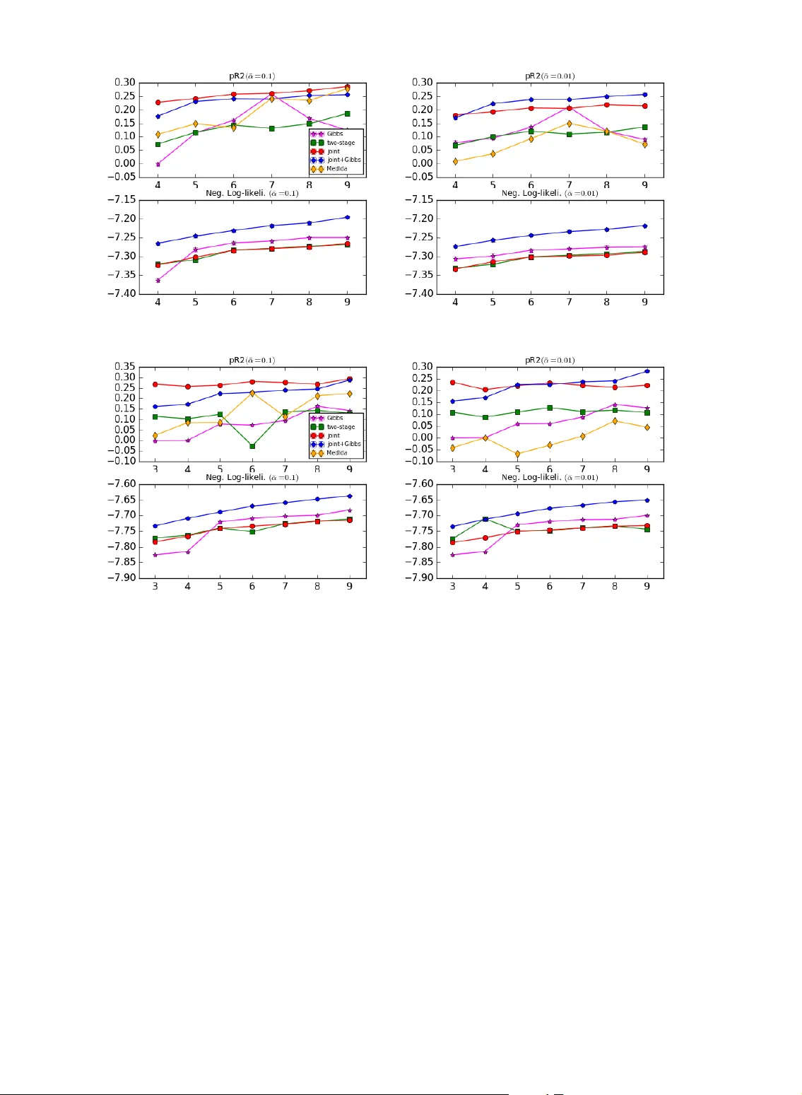
JOURNAL OF L A T E X CLASS FILES, V OL. 6, NO . 1, JANU ARY 2007 1 Spectral Lear ning f or Super vised T opic Models Y ong Ren ‡ , Yining W ang ‡ , Jun Zhu, Member , IEEE Abstract —Supervised topic models simultaneously model the latent topic structure of large collections of documents and a response variab le associated with each document. Existing inference methods are based on v ar iational appro ximation or Monte Carlo sampling, which often suffers from the local minimum defect. Spectral methods have been applied to lear n unsuper vised topic models, such as latent Dirichlet allocation (LD A), with provab le guarantees. This paper investigates the possibility of applying spectral methods to recov er the parameters of supervised LD A (sLD A). We ﬁrst present a two-stage spectral method, which recov ers the parameters of LD A follo wed by a power update method to recov er the regression model parameters. Then, we fur ther present a single-phase spectral algorithm to jointly recover the topic distribution matrix as well as the regression weights. Our spectral algorithms are provab ly correct and computationally efﬁcient. W e prove a sample complexity bound for each algor ithm and subsequently derive a sufﬁcient condition for the identiﬁability of sLDA. Thorough experiments on synthetic and real-world datasets verify the theor y and demonstrate the practical eff ectiveness of the spectral algor ithms. In f act, our results on a large-scale review rating dataset demonstrate that our single-phase spectral algor ithm alone gets comparable or e ven better performance than state-of-the-ar t methods, while previous work on spectral methods has rarely repor ted such promising performance. Index T erms —spectral methods, supervised topic models, methods of moments F 1 I N T R O D U C T I O N T O P I C modeling offers a suite of useful tools that automatically learn the latent semantic structur e of a large collection of documents or images, with latent Dirichlet allocation (LDA) [11] as one of the most popular examples. The vanilla LDA is an unsu- pervised model built on input contents of documents or images. In many applications side information is often available apart from raw contents, e.g., user- provided rating scores of an online review text or user-generated tags for an image. Such side signal usually provides additional information to r eveal the underlying structures of the data in study . There have been extensive studies on developing topic models that incorporate various side information, e.g., by treating it as supervision. Some representative models are supervised LDA (sLDA) [10] that captures a real- valued regr ession response for each document, multi- class sLDA [28] that learns with discrete classiﬁcation responses, discriminative LDA (DiscLDA) [18] that incorporates classiﬁcation response via discriminative linear transformations on topic mixing vectors, and MedLDA [32], [33] that employs a max-margin cri- • ‡ Y .R. and Y .W . contributed equally. • Y . Ren and J. Zhu are with Department of Computer Science and T echnology; TNList Lab; State Key Laboratory for Intelli- gent T echnology and Systems; Center for Bio-Inspired Comput- ing Research, T singhua University , Beijing, 100084 China. Email: reny11@mails.tsinghua.edu.cn; dcszj@tsinghua.edu.cn. • Y . Wang is with Machine Learning Department, Carnegie Mellon University , Pittsburgh, USA. Email: yiningwa@andrew .cmu.edu terion to learn discriminative latent topic repr esenta- tions for accurate prediction. T opic models are typically learned by ﬁnding maxi- mum likelihood estimates (MLE) thr ough local sear ch or sampling methods [15], [24], [25], which may get trapped in local optima. Much recent progress has been made on developing spectral decomposition [1], [3], [5] and nonnegative matrix factorization (NMF) [6], [7], [8], [9] methods to estimate the topic-wor d dis- tributions. Instead of ﬁnding MLE estimates, which is a known NP-hard problem [8], these methods assume that the documents are i.i.d. sampled from a topic model, and attempt to recover the underlying model parameters. Compared to local search and sampling algorithms, these methods enjoy the advantage of being provably effective. In fact, sample complexity bounds have been proved to show that given a sufﬁ- ciently large collection of documents, these algorithms can recover the model parameters accurately with a high probability . Recently , some attention has been paid on super- vised topic models with NMF methods. For example, Nguyen et al. [23] pr esent an extension of the anchor- word methods [6] for LDA to capture categorical information in a supervised LDA for sentiment clas- siﬁcation. However , for spectral methods, previous work has mainly focused on unsupervised latent vari- able models, leaving the broad family of supervised models (e.g., sLDA) largely unexplored. The only exception is [12] which presents a spectral method for mixtures of r egression models, quite dif ferent fr om sLDA. Such ignorance is not a coincidence as super- JOURNAL OF L A T E X CLASS FILES, V OL. 6, NO . 1, JANU ARY 2007 2 vised models impose new technical challenges. For in- stance, a direct application of previous techniques [1], [3] on sLDA cannot handle regr ession models with duplicate entries. In addition, the sample complexity bound gets much worse if we try to match entries in regression models with their corresponding topic vectors. In this paper , we extend the applicability of spec- tral learning methods by presenting novel spectral decomposition algorithms to recover the parameters of sLDA models from low-or der empirical moments estimated from the data. W e present two variants of spectral methods. The ﬁrst algorithm is an extension of the spectral methods for LDA, with an extra power update step of recovering the regression model in sLDA, including the variance parameter . The power- update step uses a newly designed empirical mo- ment to recover r egression model entries dir ectly from the data and reconstructed topic distributions. It is free from making any constraints on the underlying regr ession model. W e provide a sample complexity bound and analyze the identiﬁability conditions. In fact, the two-stage method does not incr ease the sam- ple complexity much compared to that of the vanilla LDA. However , the two-stage algorithm could have some disadvantages because of its separation that the topic distribution matrix is recover ed in an unsupervised manner without considering supervision and the re- gression parameters are recover ed by assuming a ﬁxed topic matrix. Such an unwarranted separation often leads to inferior performance compared to Gibbs sampling methods in practice (See Section 7). T o ad- dress this problem, we further present a novel single- phase spectral method for supervised topic models, which jointly recovers all the model parameters (ex- cept the noise variance) by doing a single-step of robust tensor decomposition of a newly designed empirical moment that takes both input data and supervision signal into consideration. Therefor e, the joint method can use supervision information in re- covering both the topic distribution matrix and r egres- sion parameters. The joint method is also provably correct and we provide a sample complexity bound to achieve the  error rate in a high probability . Finally , we provide thorough experiments on both synthetic and r eal datasets to demonstrate the practi- cal effectiveness of our spectral methods. For the two- stage method, by combining with a Gibbs sampling procedur e, we show superior performance in terms of language modeling, prediction accuracy and running time compar ed to traditional inference algorithms. Furthermore, we demonstrate that on a large-scale review rating dataset our single-phase method alone can achieve comparable or even better results than the state-of-the-art methods (e.g., sLDA with Gibbs sampling and MedLDA). Such promising r esults are signiﬁcant to the literature of spectral methods, which were often observed to be inferior to the MLE-based methods; and a common heuristic was to use the outputs of a spectral method to initialize an EM algorithm, which sometimes improves the perfor- mance [31]. The r est of the paper is organized as follows. Section 2 reviews basics of supervised topic models. Section 3 introduces the background knowledge and notations for sLDA and high-order tensor decomposition. Sec- tion 4 pr esents the two-stage spectral method, with a rigorous theoretical analysis, and Section 5 presents the joint spectral method together with a sample complexity bound. Section 6 presents some implemen- tation details to scale up the computation. Section 7 presents experimental results on both synthetic and real datasets. Finally , we conclude in Section 8 . 2 R E L A T E D W O R K Based on differ ent principles, there ar e various meth- ods to learn supervised topic models. The most nat- ural one is maximum-likelihood estimation (MLE). However , the highly non-convex property of the learning objective makes the optimization problem very hard. In the original paper [10], where the MLE is used, the authors choose variational approximation to handle intractable posterior expectations. Such a method tries to maximize a lower bound which is built on some variational distributions and a mean- ﬁeld assumption is usually imposed for tractability . Although the method works well in practice, we do not have any guarantee that the distribution we learned is close to the true one. Under Bayesian frame- work, Gibbs sampling is an attractive method which enjoys the pr operty that the stationary distribution of the chain is the target posterior distribution. However , this does not mean that we can really get accurate samples from posterior distribution in practice. The slow mixing rate often makes the sampler trapped in a local minimum which is far from the true distribution if we only run a ﬁnite number of iterations. Max-margin learning is another principle on learn- ing supervised topic models, with maximum entropy discrimination LDA (MedLDA) [32] as a popular ex- ample. MedLDA explores the max-margin principle to learn sparse and discriminative topic repr esenta- tions. The learning problem can be deﬁned under the regularized Bayesian infer ence (RegBayes) [34] frame- work, where the max-margin posterior regularization is introduced to ensure that the topic repr esentations are good at predicting response variables. Though both carefully designed variational inference [32] and Gibbs sampling methods [33] are given, we still can- not guarantee the quality of the learnt model in general. Recently , increasing efforts have been made to re- cover the parameters directly with provable correct- ness for topic models, with the main focus on unsu- pervised models such as LDA. Such methods adopt JOURNAL OF L A T E X CLASS FILES, V OL. 6, NO . 1, JANU ARY 2007 3 either NMF or spectral decomposition approaches. For NMF , the basic idea is that even NMF is an NP- hard problem in general, the topic distribution matrix can be recover ed under some separable condition, e.g., each topic has at least one anchor word. Precisely , for each topic, the method ﬁrst ﬁnds an anchor word that has non-zero probability only in that topic. Then a recovery step r econstructs the topic distribution given such anchor words and a second-order moment ma- trix of word-word co-occurr ence [8], [6]. The original reconstr uction step only needs a part of the matrix which is not r obust in practice. Thus in [6], the author recovers the topic distribution based on a probabilistic framework. The NMF methods produce good empiri- cal results on real-world data. Recently , the work [23] extends the anchor word methods to handle super- vised topic models. The method augments the word co-occurrence matrix with additional dimensions for metadata such as sentiment, and shows better perfor- mance in sentiment classiﬁcation. Spectral methods start fr om computing some low- order moments based on the samples and then r elate them with the model parameters. For LDA, tensors up to three order are sufﬁcient to r ecover its pa- rameters [1]. After centralization, the moments can be expressed as a mixture of the parameters we are interested in. After that whitening and r obust tensor decomposition steps are adopted to recover model parameters. The whitening step makes that the third-or der tensor can be decomposed as a set of orthogonal eigenvectors and their corresponding eigenvalues after some operations based on its output and the robust tensor decomposition step then ﬁnds them. Previous work only focuses on unsupervised LDA models and we aim to extend the ability for spectral methods to handle r esponse variables. Finally , some preliminary results of the two-stage recovery algorithm have been reported in [29]. This paper presents a systematical analysis with a novel one- stage spectral method, which yields promising r esults on a large-scale dataset. 3 P R E L I M I N A R I E S W e ﬁrst overview the basics of sLDA, orthogonal tensor decomposition and the notations to be used. 3.1 Supervised LD A Latent Dirichlet allocation (LDA) [11] is a hierarchical generative model for topic modeling of text docu- ments or images r epresented in a bag-of-visual-wor ds format [20]. It assumes k differ ent topics with topic- word distributions µ 1 , · · · , µ k ∈ ∆ V − 1 , where V is the vocabulary size and ∆ V − 1 denotes the probability simplex of a V -dimensional random vector . For a document, LDA models a topic mixing vector h ∈ ∆ k − 1 as a probability distribution over the k topics. A conjugate Dirichlet prior with parameter α is imposed α h z µ x y η y = η > h +  M N Fig. 1. A graphical illustration of super vised LDA. See te xt for details . on the topic mixing vectors. A bag-of-words model is then adopted, which ﬁrst generates a topic indicator for each word z j ∼ Multi ( h ) and then generates the word itself as w j ∼ Multi ( µ z j ) . Supervised latent Dirichlet allocation (sLDA) [10] incorporates an extra response variable y ∈ R for each document. The response variable is modeled by a linear regr ession model η ∈ R k on either the topic mixing vector h or the averaging topic assignment vector ¯ z , where ¯ z i = 1 M P M j =1 1 [ z j = i ] with M being the number of words in the document and 1 [ · ] being the indicator function (i.e., equals to 1 if the predicate holds; oth- erwise 0). The noise is assumed to be Gaussian with zero mean and σ 2 variance. Fig. 1 shows the graph structure of the sLDA model using h for regr ession. Although pr evious work has mainly focused on the model using averaging topic assignment vector ¯ z , which is convenient for col- lapsed Gibbs sampling and variational inference with h integrated out due to the conjugacy between a Dirichlet prior and a multinomial likelihood, we con- sider using the topic mixing vector h as the features for regr ession because it will considerably simplify our spectral algorithm and analysis. One may assume that whenever a document is not too short, the empir- ical distribution of its word topic assignments should be close to the document’s topic mixing vector . Such a scheme was adopted to learn sparse topic coding models [35], and has demonstrated promising results in practice. Our results also prove that this is an effective strategy . 3.2 High-order tensor product and or thogonal tensor decomposition Here we brieﬂy introduce something about tensors, which mostly follow the same as in [3]. A real p - th order tensor A ∈ N p i =1 R n i belongs to the tensor product of Euclidean spaces R n i . W ithout loss of generality , we assume n 1 = n 2 = · · · = n p = n . W e can identify each coordinate of A by a p -tuple ( i 1 , · · · , i p ) , where i 1 , · · · , i p ∈ [ n ] . For instance, a p -th order tensor is a vector when p = 1 and a matrix when p = 2 . W e can also consider a p -th order tensor A as a multilinear mapping. For A ∈ N p R n and matrices X 1 , · · · , X p ∈ R n × m , the mapping A ( X 1 , · · · , X p ) is a p -th or- der tensor in N p R m , with [ A ( X 1 , · · · , X p )] i 1 , ··· ,i p , P j 1 , ··· ,j p ∈ [ n ] A j 1 , ··· ,j p [ X 1 ] j 1 ,i 1 [ X 2 ] j 2 ,i 2 · · · [ X p ] j p ,i p . Con- sider some concrete examples of such a multilinear JOURNAL OF L A T E X CLASS FILES, V OL. 6, NO . 1, JANU ARY 2007 4 mapping. When A , X 1 and X 2 are matrices, we have A ( X 1 , X 2 ) = X > 1 AX 2 . Similarly , when A is a matrix and x is a vector , we have A ( I , x ) = Ax . An orthogonal tensor decomposition of a tensor A ∈ N p R n is a collection of orthonormal vectors { v i } k i =1 and scalars { λ i } k i =1 such that A = P k i =1 λ i v ⊗ p i , where we use v ⊗ p , v ⊗ v ⊗ · · · ⊗ v to denote the p -th order tensor generated by a vector v . W ithout loss of generality , we assume λ i are nonnegative when p is odd since we can change the sign of v i otherwise. Al- though orthogonal tensor decomposition in the matrix case can be done efﬁciently by singular value decom- position (SVD), it has several delicate issues in higher order tensor spaces [3]. For instance, tensors may not have unique decompositions, and an orthogonal decomposition may not exist for every symmetric ten- sor [3]. Such issues are further complicated when only noisy estimates of the desired tensors are available. For these reasons, we need more advanced techniques to handle high-order tensors. In this paper , we will apply robust tensor power methods [3] to r ecover robust eigenvalues and eigenvectors of an (estimated) third- order tensor . The algorithm recovers eigenvalues and eigenvectors up to an absolute err or ε , while running in polynomial time w .r .t the tensor dimension and log(1 /ε ) . Further details and analysis of the robust tensor power method are in Appendix A.2 and [3]. 3.3 Notations W e use k v k = p P i v 2 i to denote the Euclidean norm of vector v , k M k to denote the spectral norm of matrix M , k T k to denote the operator norm of a high- order tensor , and k M k F = q P i,j M 2 ij to denote the Frobenious norm of M . W e use an one-hot vector x ∈ R V to r epresent a word in a document (i.e., for the i -th word in a vocabulary , only x i = 1 all other elements are 0 ). In the two-stage spectral method, we use O , ( µ 1 , µ 2 , · · · , µ k ) ∈ R V × k to denote the topic distribution matrix, and e O , ( e µ 1 , e µ 2 , · · · , e µ k ) to denote the canonical version of O , where e µ i = q α i α 0 ( α 0 +1) µ with α 0 , P k i =1 α i . For the joint spec- tral method, we combine the topic distribution µ i with its regression parameter to form a joint topic distribution vector v i , [ µ 0 i , η i ] 0 . W e use notation O ∗ , ( v 1 , v 2 , ..., v k ) ∈ R ( V +1) × k to denote the joint topic distribution matrix and e O ∗ , [ e v 1 , e v 2 , ..., e v k ] to denote its canonical version where e v i , q α i α 0 ( α 0 +1) v i . 4 A T W O - S TAG E S P E C T R A L M E T H O D W e ﬁrst present a two-stage spectral method to re- cover the parameters of sLDA. The algorithm consists of two key components—an orthogonal tensor decom- position of observable moments to recover the topic distribution matrix O and a power update method to recover the regr ession model η . W e present these techniques and a rigorous theoretical analysis below . 4.1 Moments of observable v ariables Our spectral decomposition methods recover the topic distribution matrix O and the linear regression model η by manipulating moments of observable variables. In Deﬁnition 1, we deﬁne a list of moments on random variables from the underlying sLDA model. Deﬁnition 1. We deﬁne the following moments of observ- able variables: M 1 = E [ x 1 ] , M 2 = E [ x 1 ⊗ x 2 ] − α 0 α 0 + 1 M 1 ⊗ M 1 , (1) M 3 = E [ x 1 ⊗ x 2 ⊗ x 3 ] − α 0 α 0 + 2 ( E [ x 1 ⊗ x 2 ⊗ M 1 ] + E [ x 1 ⊗ M 1 ⊗ x 2 ] + E [ M 1 ⊗ x 1 ⊗ x 2 ]) + 2 α 2 0 ( α 0 + 1)( α 0 + 2) M 1 ⊗ M 1 ⊗ M 1 , (2) M y = E [ y x 1 ⊗ x 2 ] − α 0 α 0 + 2 ( E [ y ] E [ x 1 ⊗ x 2 ] + E [ x 1 ] ⊗ E [ y x 2 ] + E [ y x 1 ] ⊗ E [ x 2 ]) + 2 α 2 0 ( α 0 + 1)( α 0 + 2) E [ y ] M 1 ⊗ M 1 . (3) Note that the moments M 1 , M 2 and M 3 were also deﬁned in [1], [3] for recovering the parameters of LDA models. For sLDA, we need to deﬁne a new moment M y in order to recover the linear regression model η . The moments are based on observable vari- ables in the sense that they can be estimated from i.i.d. sampled documents. For instance, M 1 can be estimated by computing the empirical distribution of all words, and M 2 can be estimated using M 1 and word co-occurr ence frequencies. Though the moments in the above forms look complicated, we can apply elementary calculations based on the conditional inde- pendence structure of sLDA to signiﬁcantly simplify them and more importantly to get them connected with the model parameters to be recover ed, as sum- marized in Proposition 1, whose proof is elementary and deferred to Appendix C for clarity . Proposition 1. The moments can be expressed using the model parameters as: M 2 = 1 α 0 ( α 0 + 1) k X i =1 α i µ i ⊗ µ i , (4) M 3 = 2 α 0 ( α 0 + 1)( α 0 + 2) k X i =1 α i µ i ⊗ µ i ⊗ µ i , (5) M y = 2 α 0 ( α 0 + 1)( α 0 + 2) k X i =1 α i η i µ i ⊗ µ i . (6) 4.2 Simultaneous dia gonalization Proposition 1 shows that the moments in Deﬁnition 1 are all the weighted sums of tensor products of { µ i } k i =1 from the underlying sLDA model. One idea to reconstruct { µ i } k i =1 is to perform simultaneous di- agonalization on tensors of different orders. The idea has been used in a number of recent developments of spectral methods for latent variable models [1], [3], [12]. Speciﬁcally , we ﬁrst whiten the second-order tensor M 2 by ﬁnding a matrix W ∈ R V × k such that JOURNAL OF L A T E X CLASS FILES, V OL. 6, NO . 1, JANU ARY 2007 5 Algorithm 1 spectral parameter recovery algorithm for sLDA. Input parameters: α 0 , L, T . 1: Compute empirical moments and obtain c M 2 , c M 3 and c M y . 2: Find c W ∈ R n × k such that c M 2 ( c W , c W ) = I k . 3: Find r obust eigenvalues and eigenvectors ( b λ i , b v i ) of c M 3 ( c W , c W , c W ) using the robust tensor power method [3] with parameters L and T . 4: Recover prior parameters: b α i ← 4 α 0 ( α 0 +1) ( α 0 +2) 2 b λ 2 i . 5: Recover topic distributions: b µ i ← α 0 + 2 2 b λ i ( c W + ) > b v i . 6: Recover the linear regr ession model: b η i ← α 0 + 2 2 b v > i c M y ( c W , c W ) b v i . 7: Output: b η , b α and { b µ i } k i =1 . W > M 2 W = I k . This whitening procedure is possible whenever the topic distribuction vectors { µ i } k i =1 are linearly independent (and hence M 2 has rank k ). This is not always correct since in the “overcomplete” case [4], it is possible that the topic number k is larger than vocabulary size V . However , the linear independent assumption gives us a more compact repr esentation for the topic model and works well in practice. Hence we simply assume that the whiten- ing procedure is possible. The whitening procedure and the linear independence assumption also imply that { W µ i } k i =1 are orthogonal vectors (see Appendix A.2 for details), and can be subsequently recovered by performing an orthogonal tensor decomposition on the simultaneously whitened third-or der tensor M 3 ( W , W, W ) . Finally , by multiplying the pseudo- inverse of the whitening matrix W + we obtain the topic distribution vectors { µ i } k i =1 . It should be noted that Jennrich’s algorithm [17], [19], [22] could recover { µ i } k i =1 directly from the 3- rd order tensor M 3 alone when { µ i } k i =1 is linearly independent. However , we still adopt the above si- multaneous diagonalization framework because the intermediate vectors { W µ i } k i =1 play a vital role in the recovery pr ocedure of the linear regression model η . 4.3 The power update method Although the linear regr ession model η can be r ecov- ered in a similar manner by performing simultaneous diagonalization on M 2 and M y , such a method has several disadvantages, thereby calling for novel so- lutions. First, after obtaining entry values { η i } k i =1 we need to match them to the topic distributions { µ i } k i =1 previously r ecovered. This can be easily done when we have access to the true moments, but becomes difﬁcult when only estimates of observable tensors are available because the estimated moments may not share the same singular vectors due to sampling noise. A more serious problem is that when η has duplicate entries the orthogonal decomposition of M y is no longer unique. Though a randomized strategy similar to the one used in [1] might solve the problem, it could substantially increase the sample complexity [3] and render the algorithm impractical. In [5], the authors pr ovide a method for the match- ing problem by reusing eigenvectors. W e here de- velop a power update method to resolve the above difﬁculties with a similar spirit. Speciﬁcally , after ob- taining the whitened (orthonormal) vectors { v i } , c i · W > µ i 1 we r ecover the entry η i of the linear re- gression model directly by computing a power update v > i M y ( W , W ) v i . In this way , the matching problem is automatically solved because we know what topic distribution vector µ i is used when recovering η i . Fur- thermore, the singular values (corresponding to the entries of η ) do not need to be distinct because we are not using any unique SVD properties of M y ( W , W ) . As a result, our proposed algorithm works for any linear model η . 4.4 P arameter recovery algorithm Alg. 1 outlines our parameter recovery algorithm for sLDA (Spectral-sLDA). First, empirical estimations of the observable moments in Deﬁnition 1 are computed from the given documents. The simultaneous diag- onalization method is then used to reconstruct the topic distribution matrix O and its prior parameter α . After obtaining O = ( µ 1 , · · · , µ k ) , we use the power update method introduced in the previous section to recover the linear regr ession model η . W e can also recover the noise level parameter σ 2 with the other parameters in hand by estimating E [ y ] and E [ y 2 ] since E [ y ] = E [ E [ y | h ]] = α > η and E [ y 2 ] = E [ E [ y 2 | h ]] = η > E [ h ⊗ h ] η + σ 2 , where the term E [ h ⊗ h ] can be computed in an analytical form using the model parameters, as detailed in Appendix C.1. Alg. 1 admits three hyper -parameters α 0 , L and T . α 0 is deﬁned as the sum of all entries in the prior parameter α . Following the conventions in [1], [3], we assume that α 0 is known a priori and use this value to perform parameter estimation. It should be noted that this is a mild assumption, as in practice usually a homogeneous vector α is assumed and the entire vector is known [27]. The L and T param- eters are used to control the number of iterations in the robust tensor power method. In general, the robust tensor power method runs in O ( k 3 LT ) time. T o ensure sufﬁcient recovery accuracy , L should be at least a linear function of k and T should be set as T = Ω(log( k ) + log log( λ max /ε )) , where λ max = 2 α 0 +2 q α 0 ( α 0 +1) α min and ε is an error tolerance parameter . Appendix A.2 and [3] provide a deeper analysis into the choice of L and T parameters. 1. c i , q α i α 0 ( α 0 +1) is a scalar coefﬁcient that depends on α 0 and α i . See Appendix A.2 for details. JOURNAL OF L A T E X CLASS FILES, V OL. 6, NO . 1, JANU ARY 2007 6 4.5 Sample Complexity Anal ysis W e now analyze the sample complexity of Alg. 1 in order to achieve ε -error with a high probability . For clarity , we focus on presenting the main results, while deferring the proof details to Appendix A, including the proofs of important lemmas that are needed for the main theorem. Theorem 1. Let σ 1 ( e O ) and σ k ( e O ) be the largest and the smallest singular values of the canonical topic dis- tribution matrix e O . Deﬁne λ min , 2 α 0 +2 q α 0 ( α 0 +1) α max and λ max , 2 α 0 +2 q α 0 ( α 0 +1) α min ? with α max and α min the lar gest and the smallest entries of α . Suppose b µ , b α and b η are the outputs of Algorithm 1, and L is at least a linear function of k . Fix δ ∈ (0 , 1) . For any small error- tolerance parameter ε > 0 , if Algorithm 1 is run with parameter T = Ω(log( k ) + log log ( λ max /ε )) on N i.i.d. sampled documents (each containing at least 3 words) with N ≥ max( n 1 , n 2 , n 3 ) , where n 1 = C 1 ·  1 + p log(6 /δ )  2 · α 2 0 ( α 0 + 1) 2 α min , n 2 = C 2 · (1 + p log(15 /δ )) 2 ε 2 σ k ( e O ) 4 · max  k η k − σ Φ − 1  δ 60  2 , α 2 max σ 1 ( e O ) 2 ! , n 3 = C 3 · (1 + p log(9 /δ )) 2 σ k ( e O ) 10 · max  1 ε 2 , k 2 λ 2 min  , and C 1 , C 2 and C 3 are universal constants, then with probability at least 1 − δ , there exists a permutation π : [ k ] → [ k ] such that for every topic i , the following holds: | α i − b α π ( i ) | ≤ 4 α 0 ( α 0 + 1)( λ max + 5 ε ) ( α 0 + 2) 2 λ 2 min ( λ min − 5 ε ) 2 · 5 ε, if λ min > 5 ε k µ i − b µ π ( i ) k ≤  3 σ 1 ( e O )  8 α max λ min + 5( α 0 + 2) 2  + 1  ε | η i − b η π ( i ) | ≤  k η k λ min + ( α 0 + 2)  ε. In brevity , the proof is based on matrix perturba- tion lemmas (see Appendix A.1) and analysis to the orthogonal tensor decomposition methods (including SVD and robust tensor power method) performed on inaccurate tensor estimations (see Appendix A.2). The sample complexity lower bound consists of three terms, from n 1 to n 3 . The n 3 term comes from the sample complexity bound for the robust tensor power method [3]; the ( k η k − σ Φ − 1 ( δ / 60)) 2 term in n 2 charac- terizes the recovery accuracy for the linear regr ession model η , and the α 2 max σ 1 ( e O ) 2 term arises when we try to recover the topic distribution vectors µ ; ﬁnally , the term n 1 is requir ed so that some technical conditions are met. The n 1 term does not depend on either k or σ k ( e O ) , and could be largely neglected in practice. Remark 1. An important implication of Theorem 1 is that it pr ovides a sufﬁcient condition for a supervised LDA model to be identiﬁable, as shown in Remark 2. T o some extent, Remark 2 is the best identiﬁability result possible under our inference framework, because it makes no restriction on the linear regr ession model η , and the linear independence assumption is unavoidable without making further assumptions on the topic distribution matrix O . Remark 2. Given a sufﬁciently large number of i.i.d. sampled documents with at least 3 words per document, a supervised LDA model M = ( α , µ , η ) is identiﬁable if α 0 = P k i =1 α i is known and { µ i } k i =1 are linearly independent. W e now take a close look at the sample complexity bound in Theorem 1. It is evident that n 2 can be neglected when the number of topics k gets large, because in practice the norm of the linear regression model η is usually assumed to be small in order to avoid overﬁtting. Moreover , as mentioned before, the prior parameter α is often assumed to be homoge- neous with α i = 1 /k [27]. W ith these observations, the sample complexity bound in Theorem 1 can be greatly simpliﬁed. Remark 3. Assume k η k and σ ar e small and α = (1 /k , · · · , 1 /k ) . As the number of topics k gets large, the sample complexity bound in Theor em 1 can be simpliﬁed as N ≥ Ω log(1 /δ ) σ k ( e O ) 10 · max( ε − 2 , k 3 ) ! . (7) The sample complexity bound in Remark 3 may look formidable as it depends on σ k ( e O ) 10 . However , such dependency is somewhat necessary because we are using thir d-order tensors to recover the underly- ing model parameters. 5 J O I N T P A R A M E T E R R E C O V E RY The above two-stage procedure has one possible dis- advantages, that is, the recovery of the topic distribu- tion matrix does not use any supervision signal, and thus the recover ed topics are often not good enough for prediction tasks, as shown in experiments. The disadvantage motivates us to develop a joint spectral method with theor etical guarantees. W e now describe our single-phase algorithm. 5.1 Moments of Observable V ariables W e ﬁrst deﬁne some moments based on the observ- able variables including the information that we need to recover the model parameters. Since we aim to recover the joint topic distribution matrix O ∗ , we combine the wor d vector x with the response variable y to form a joint vector z = [ x 0 , y ] 0 and deﬁne the following moments: JOURNAL OF L A T E X CLASS FILES, V OL. 6, NO . 1, JANU ARY 2007 7 Fig. 2. Interaction between response variable y and word v ector x in the 3rd-order tensor M 3 . Deﬁnition 2. (Centerized Moments) N 1 = E [ z 1 ] N 2 = E [ z 1 ⊗ z 2 ] − α 0 α 0 + 1 N 1 ⊗ N 1 − σ 2 e ⊗ e N 3 = E [ z 1 ⊗ z 2 ⊗ z 3 ] − α 0 α 0 + 1 ( E [ z 1 ⊗ z 2 ⊗ N 1 ] + E [ z 1 ⊗ N 1 ⊗ z 2 ] + E [ N 1 ⊗ z 1 ⊗ z 2 ]) + 2 α 2 0 ( α 0 + 1)( α 0 + 2) N 1 ⊗ N 1 ⊗ N 1 + 3 σ 2 N 1 V +1 e ⊗ e ⊗ e + 1 α 0 + 1 σ 2 ( e ⊗ e ⊗ N 1 + e ⊗ N 1 ⊗ e + N 1 ⊗ e ⊗ e ) , (8) where e is the ( V + 1) -dimensional vector with the last element equaling to 1 and all others zero, N 1 V +1 is the V + 1 -th element of N 1 . The intuition for such deﬁnitions is derived from an important observation that once the latent vari- able h is given, the mean value of y is a weighted combination of the regression parameters and h (i.e., E [ y | h ] = P k i =1 η i h i ), which has the same form as for x (i.e., E [ x | h ] = P k i =1 µ i h i ). Therefore, it is nat- ural to regar d y as an additional dimension of the word vector x , which gives the new vector z . This combination leads to some other terms involving the high-order moments of y , which introduce the vari- ance parameter σ when we centerize the moments. Although we can recover σ in the two-stage method, recovering it jointly with the other parameters seems to be har d. Thus we treat σ as a hyper-parameter . One can determine it via a cross-validation pr ocedure. As illustrated in Fig. 2, our 3rd-order moment can be viewed as a centerized version of the combination of N 0 3 , E [ x 1 ⊗ x 2 ⊗ x 3 ] , N 0 y , E [ y x 2 ⊗ x 2 ] and some high-order statistics of the response variables. Note that this combination has already aligned the regr ession parameters with the corresponding topics. Hence, we do not need an extra matching step. In practice, we cannot get the exact values of those moments. Instead, we estimate them from the i.i.d. sampled documents. Note that we only need the moments up to the third order , which means any document consisting of at least three words can be used in this estimation. Furthermore, although these moments seem to be complex, they can be expressed via the model parameters in a graceful manner , as summarized in Pr oposition 2 which can be proved by expanding the terms by deﬁnition, similar as in the proof of Proposition 1. Algorithm 2 a joint spectral method to recover sLDA parameters. Input parameters: α 0 , L , T , σ 1: Compute empirical moments and obtain b N 2 , c N 3 . 2: Find c W ∈ R V +1 × k such that b N 2 ( c W , c W ) = I k . 3: Find r obust eigenvalues and eigenvectors ( b λ i , b v i ) of b N 3 ( c W , c W , c W ) using the robust tensor power method with parameters L and T . 4: Recover prior parameters: b α i ← 4 α 0 ( α 0 +1) ( α 0 +2) 2 b λ 2 i . 5: Recover topic distribution: b v i ← α 0 + 2 2 b λ i ( W + ) > b ω i . 6: Output: model parameters b α i , b v i i = 1 , ..., k Proposition 2. The moments in Deﬁnition 2 can be expressed by using the model parameters as follows: N 2 = 1 α 0 ( α 0 + 1) k X i =1 α i v i ⊗ v i N 3 = 2 α 0 ( α 0 + 1)( α 0 + 2) k X i =1 α i v i ⊗ v i ⊗ v i , (9) where v i is the concatenation of the i -th word-topic distri- bution µ i and regr ession parameter η i . 5.2 Robust T ensor Decomposition Proposition 2 shows that the centerized tensors are weighted sums of the tensor products of the param- eters { v i } k i =1 to be recovered. A similar procedure as in the two-stage method can be followed in order to develop our joint spectral method, which consists of whitening and robust tensor decomposition steps. First, we whiten the 2nd-order tensor N 2 by ﬁnding a matrix W ∈ R ( V +1) × k such that W > N 2 W = I k . This whitening procedur e is possible whenever the joint topic distribution vectors { v i } k i =1 are linearly indepen- dent, that is, the matrix has rank k . The whitening procedur e and the linear independence assumption also imply that { W > v i } k i =1 are orthogonal vectors and can be subsequently recover ed by performing an orthogonal tensor decomposition on the simulta- neously whitened third-or der tensor N 3 ( W , W, W ) as summarized in the following proposition. Proposition 3. Deﬁne ω i = r α i α 0 ( α 0 + 1) W > v i . Then: • { ω } k i =1 is an orthonormal basis. • N 3 ( W , W, W ) has pairs of robust eigenvalue and eigenvector ( λ i , v i ) with λ = 2 α 0 + 2 r α 0 ( α 0 + 1) α i Finally , by multiplying the pseudo-inverse of the whitening matrix W + we obtain the joint topic distri- bution vectors { v i } k i =1 . W e outline our single-phase spectral method in Alg. 2. Here we assume that the noise variance σ is given. Note that in the two-stage spectral method, it JOURNAL OF L A T E X CLASS FILES, V OL. 6, NO . 1, JANU ARY 2007 8 does not need the parameter σ because it does not use the information of the variance of prediction error . Although there is a disadvantage that we need to tune it, the introduction of σ sometimes incr eases the ﬂexibility of our methods on incorporating some prior knowledge (if exists). W e additionally need three hyper-parameters α 0 , L and T , similar as in the two-stage method. The pa- rameter α 0 is deﬁned as the summation of all the entries of the prior parameter α . L and T are used to control the number of iterations in robust tensor decomposition. T o ensure a suf ﬁciently high recovery accuracy , L should be at least a linear function of k , and T should be set as T = Ω(log ( k )+ log log( λ max / )) , where λ max = 2 α 0 +2 q α 0 ( α 0 +1) α min and  is the error rate. 5.3 Sample Complexity Anal ysis W e now analyze the sample complexity in order to achieve  -error with a high pr obability . For clarity , we defer proof details to Appendix B. Theorem 2. Let σ 1 ( e O ∗ ) and σ k ( e O ∗ ) be the largest and smallest singular values of the joint canonical topic distribution matrix e O ∗ . Let λ max , 2 α 0 +2 q α 0 ( α 0 +1) α min where α min is the smallest element of α ; λ min , 2 α 0 +2 q α 0 ( α 0 +1) α max where α max is the largest element of α . For any err or-tolerance parameter  > 0 , if Algorithm 2 runs at least T = Ω(log ( k ) + log log( λ max / )) iterations on N i.i.d. sampled documents with N ≥ ( n 0 1 , n 0 2 , n 0 3 ) , where: n 0 1 = K 1 · α 2 0 ( α 0 + 1) 2 C 2 ( δ / 36 N ) · (2 + p 2 log (18 /δ )) 2 α 2 min n 0 2 = K 2 · C 2 ( δ / 144 N )(2 + p 2 log (72 /σ )) 2 n 0 3 = K 3 · C 2 ( δ / 36 N )(2 + p 2 log (18 /σ )) 2 σ k ( e O ∗ ) 10 · max( 1  2 , k 2 λ 2 min ) , C ( x ) is a polynomial of inverse CDF of normal distribution and the norm of regr ession parameters k η k ; K 1 , K 2 , K 3 are some universal constants. Then with probability at least 1 − δ , there exist a permutation π : [ k ] → [ k ] such that the following holds for every i ∈ [ k ] : | α i − b α π ( i ) | ≤ 4 α 0 ( α 0 + 1) ( α 0 + 2) 2 λ 2 min ( λ min − 5  ) 2 · 5  k v i − b v π ( i ) k ≤  σ 1 ( e O ∗ )( α 0 + 2)( 7 2 + 8 λ min )  · . Similar to Theorem 1, the sample complexity bound consists of three terms. The ﬁrst and second terms do not depend on the error rate  , which are required so that some technical conditions are met. Thus they could be largely neglected in practice. The third n 0 3 term comes from the sample complexity bound for the robust tensor power method [3]. Remark 4. Note the RHS of the requir ements of N includes a function of N (i.e., C (1 / N ) ). As mentioned above, C ( x ) is polynomial of inverse CDF of normal distribution with low degree. Since the inverse CDF gr ows very slowly (i.e., | Φ − 1 (1 / N ) | = o (log ( N )) ). We can omit it safely . Remark 5. Following the above remark and assume that k η k and σ are small and α are homogeneous, the sample complexity can be simpliﬁed as (a function of k ): N = O log(1 /σ ) σ k ( e O ∗ ) 10 · max( 1  2 , k 3 ) ! . The factor 1 /σ k ( e O ∗ ) 10 is large, however , such a fac- tor is necessary since we use the third order tensors. This factor r oots in the tensor decomposition methods and one can expect to improve it if we have other better methods to decompose b N 3 . 5.4 Sample Complexity Comparison As mentioned in Remark 3 and Remark 5, the joint spectral method shares the same sample complexity as the two-stage algorithm in order to achieve  accuracy , except two minor differences. First, the sample complexity depends on the small- est singular value of (joint) topic distribution σ k ( e O ) . For the joint method, the joint topic distribution ma- trix consists of the original topic distribution matrix and one extra row of the r egression parameters. Thus from W eyl’s inequality [30], the smallest singular value of the joint topic distribution matrix is larger than that of the original topic distribution matrix, and then the sample complexity of the joint method is a bit lower than that of the two-stage method, as empirically justiﬁed in experiments. Second, dif ferent fr om the two-stage method, the er- rors of topic distribution µ and regr ession parameters η ar e estimated together in the joint method (i.e., v ), which can potentially give more accurate estimation of regr ession parameters considering that the number of regression parameters is much less than the topic distribution. 6 S P E E D I N G U P M O M E N T C O M P U T AT I O N W e now analyze the computational complexity and present some implementation details to make the algorithms more efﬁcient. 6.1 T wo-Stage Method In Alg. 1, a straightforward computation of the third- order tensor c M 3 requir es O ( N M 3 ) time and O ( V 3 ) storage, where N is corpus size, M is the number of words per document and V is the vocabulary size. Such time and space complexities are clearly prohibitive for real applications, wher e the vocab- ulary usually contains tens of thousands of terms. However , we can employ a trick similar as in [13] to speed up the moment computation. W e ﬁrst note that only the whitened tensor c M 3 ( c W , c W , c W ) is needed in our algorithm, which only takes O ( k 3 ) storage. Another observation is that the most difﬁcult term JOURNAL OF L A T E X CLASS FILES, V OL. 6, NO . 1, JANU ARY 2007 9 in c M 3 can be written as P r i =1 c i u i, 1 ⊗ u i, 2 ⊗ u i, 3 , where r is proportional to N and u i, · contains at most M non-zero entries. This allows us to compute c M 3 ( c W , c W , c W ) in O ( N M k ) time by com- puting P r i =1 c i ( W > u i, 1 ) ⊗ ( W > u i, 2 ) ⊗ ( W > u i, 3 ) . Ap- pendix C.2 pr ovides more details about this speed-up trick. The overall time complexity is O ( N M ( M + k 2 ) + V 2 + k 3 LT ) and the space complexity is O ( V 2 + k 3 ) . 6.2 Joint Method For the single-phase algorithm, a straightforward computation of the thir d-order tensor b N 3 has the same complexity of O ( N M 3 ) as in the two-stage method. And a much higher time complexity is needed for computing b N 3 ( c W , c W , c W ) , which is prohibitive. Sim- ilar as in the two-stage method, since we only need b N 3 ( c W , c W , c W ) in Alg. 2, we turn to compute this term directly . W e can then use the trick mentioned above to do this. The key idea is to decompose the thir d-order tensor into different parts based on the occurrence of words and compute them respectively . The same time comlexity and space complexity is needed for the single-phase method. Sometimes N 2 and N 3 are not “balanced” (i.e., the value of some elements are much larger than the others). This situation happens when either the vocabulary size is too large or the range of η is too large. One can image that if we have a vocabulary consisting of one million words while min η i = 1 , then the energy of the matrix N 2 concentrates on ( N 2 ) V +1 ,V +1 . As a consequence, the SVD performs badly when the matrix is ill-conditioned. A practical solution to this problem is that we scale the word vector x by a constant, that is, for the i -th word in the dictionary , we set x i = C , x j = 0 , ∀ i 6 = j , where C is a constant. The main effect is that we can make the matrix more stable after this manipulation. Note that when we ﬁx C , this makes no effect on the recovery accuracy . Such a trick is primarily for computational stability . In our experiments, C is set to be 100 . 6.3 Dealing with large v ocabulary size V One key step in the whitening procedure of both methods is to perform SVD on the second order moment M 2 ∈ R V × V (or N 2 ∈ R ( V +1) × ( V +1) ). A straightforward implementation of SVD has complex- ity O ( k V 2 ) , 2 which is unbearable when the vocabu- lary size V is large. W e follow the method in [14] and perform random projection to reduce dimensionality . More precisely , let S ∈ R e k where e k < V be a random matrix and then deﬁne C = M 2 S and Ω = S > M 2 S . Then a low rank approximation of M 2 is given by f M 2 = C Ω + C > . Now we can obtain the whitening matrix without directly performing an SVD on M 2 by appoximating C − 1 and Ω separately . The overall 2. It is not O ( V 3 ) as we only need top- k truncated SVD. Algorithm 3 Randomized whitening procedure. Input parameters: second order moment M 2 (or N 2 ). 1: Generate a random projection matrix S ∈ R V × e k . 2: Compute the matrices C and Ω : C = M 2 S ∈ R V × e k , and Ω = S > M 2 S ∈ R e k × e k . 3: Do SVD for both C and Ω : C = U C Σ C D > C , and Ω = U Ω Σ Ω D > Ω 4: T ake the rank- k appr oximation: U C ← U C ( : , 1 : k ) Σ C ← Σ C (1 : k , 1 : k ) , D C ← D C ( : , 1 : k ) D Ω ← D Ω (1 : k , 1 : k ) , Σ Ω ← Σ Ω (1 : k , 1 : k ) 5: Whiten the approximated matrix: W = U C Σ − 1 C D > C D Ω Σ 1 / 2 Ω . 6: Output: Whitening matrix W . algorithm is provided in Alg. 3. In practice, we set e k = 10 k to get a sufﬁciently accurate approximation. 7 E X P E R I M E N T S W e now present experimental results on both syn- thetic and two real-world datasets. For our spectral methods, the hyper-parameters L and T are set to be 100 , which is sufﬁciently lar ge for our experiment settings. Since spectral methods can only recover the underlying parameters, we ﬁrst run them to recover those parameters in training and then use Gibbs sam- pling to infer the topic mixing vectors h and topic assignments for each word t i for testing. Our main competitor is sLDA with a Gibbs sampler (Gibbs-sLDA), which is asymptotically accurate and often outperforms variational methods. W e imple- ment an uncollapsed Gibbs sampler , which alternately draws samples from the local conditionals of η , z , h , or µ , when the rest variables are given. W e monitor the behavior of the Gibbs sampler by observing the relative change of the training data log-likelihood, and terminate when the average change is less than a given threshold (e.g., 1 e − 3 ) in the last 10 iterations. The hyper-parameters of the Gibbs sampler are set to be the same as our methods, including topic numbers and α . W e evaluate a hybrid method that uses the parameters µ , η , α recovered by our joint spectral method as initialization for a Gibbs sampler . This strategy is similar to that in [31], where the estimation of a spectral method is used to initialize an EM method for further reﬁning. In our hybrid method, the Gibbs sampler plays the similar role of reﬁning. W e also compare with MedLDA [32], a state-of-the- art topic model for classiﬁcation and regr ession, on real datasets. W e use the Gibbs sampler with data augmentation [33], which is more accurate than the original variational methods, and adopts the same stopping condition as above. On the synthetic data, we ﬁrst use L 1 -norm to measure the difference between the reconstructed pa- rameters and the underlying true parameters. Then we compare the prediction accuracy and per-word JOURNAL OF L A T E X CLASS FILES, V OL. 6, NO . 1, JANU ARY 2007 10 likelihood on both synthetic and real-world datasets. The quality of the prediction on the synthetic dataset is measured by mean squared error (MSE) while the quality on the real-wor d dataset is assessed by predictive R 2 ( pR 2 ), a normalized version of MSE, which is deﬁned as pR 2 = 1 − P i ( y i − b y i ) 2 P i ( y i − ¯ y ) 2 , where ¯ y is the mean of testing data and b y i is the estimation of y i . The per-wor d log-likelihood is deﬁned as log p ( ω | h , O ) = log P k j =1 p ( ω | t = j, O ) p ( t = j | h ) . 7.1 Synthetic Dataset W e generate our synthetic dataset following the gen- erative process of sLDA, with a vocabulary of size V = 500 and topic number k = 20 . W e generate the topic distribution matrix O by ﬁrst sampling each en- try from a uniform distribution and then normalizing every column of it. The linear regression model η is sampled from a standard Gaussian distribution. The prior parameter α is assumed to be homogeneous, i.e., α = (1 /k , ..., 1 /k ) . Documents and response variables are then generated fr om the sLDA model speciﬁed in Section 3.1. W e consider two cases where the length of each document is set to be 250 and 500 repectively . The hyper-parameters are set to be the same as the ones that used to generate the dataset 3 . 7.1.1 Conv ergence of estimated model parameters Fig. 3 and Fig. 4 show the L 1 -norm reconstruction er- rors of α , η and µ when each document contains dif- ferent number of words. Note that due to the uniden- tiﬁability of topic models, we only get a permutated estimation of the underlying parameters. Thus we run a bipartite graph matching to ﬁnd a permutation that minimizes the reconstruction error . W e can ﬁnd that as the sample size increases, the r econstruction errors for all parameters decr ease consistently to zer o in both methods, which veriﬁes the correctness of our theory . T aking a closer look at the ﬁgures, we can see that the empirical convergence rates for α and µ are almost the same for the two spectral methods. However , the convergence rate for regression parameters η in the joint method is much higher than the one in the two- stage method, as mentioned in the comparison of the sample complexity in Section 5.4 , due to the fact that the joint method can bound the estimation error of η and µ together . Furthermore, though Theorem 1 and Theorem 2 do not involve the number of words per document, the simulation results demonstrate a signiﬁcant improve- ment when more wor ds are observed in each docu- ment, which is a nice complement for the theoretical analysis. 3. The methods ar e insensitive to the hyper-parameters in a wide range. e.g., we still get high accuracy even we set the hyper- parameter α 0 to be twice as large as the true value. Fig. 5. Mean square errors and negative per-word log- likelihood of Alg. 1 and Gibbs sLD A. Each document contains M = 500 words . The X axis denotes the training size ( × 10 3 ). The ”ref. model” denotes the one with the underlying tr ue parameters . 7.1.2 Prediction accuracy and per-word likelihood Fig. 5 shows that both spectral methods consistently outperform Gibbs-sLDA. Our methods also enjoy the advantage of being less variable, as indicated by the curve and error bars. Moreover , when the number of training documents is sufﬁciently large, the per- formance of the reconstructed model is very close to the true model 4 , which implies that our spectral methods can correctly identify an sLDA model from its observations, therefore supporting our theory . The performances of the two-stage spectral method and the joint one are comparable this time, which is largely because of the fact the when giving enough training data, the r ecovered model is accurate enough. The Gibbs method is easily caught in a local minimum so we can ﬁnd as the sample size increases, the prediction err ors do not decrease monotonously . Fig. 6. pR 2 scores and negative per-word log- likelihood on the Hotel Revie w dataset. The X axis indicates the number of topics . Error bars indicate the standard de viation of 5 -fold cross-v alidation. 4. Due to the randomness in the data generating process, the true model has a non-zero pr ediction error . JOURNAL OF L A T E X CLASS FILES, V OL. 6, NO . 1, JANU ARY 2007 11 Fig. 3. Reconstr uction errors of two spectral methods when each document contains 250 words. X axis denotes the training size n in log domain with base 2 (i.e., n = 2 k , k ∈ { 8 , ..., 15 } ). Error bars denote the standard de viations measured on 3 independent tr ials under each setting. Fig. 4. Reconstr uction errors of two spectral methods when each document contains 500 words. X axis denotes the training size n in log domain with base 2 (i.e., n = 2 k , k ∈ { 8 , ..., 15 } ). Error bars denote the standard de viations measured on 3 independent tr ials under each setting. 7.2 Hotel Revie ws Dataset For real-world datasets, we ﬁrst test on a relatively small Hotel Review dataset, which consists of 15 , 000 documents for training and 3 , 000 documents for testing that are randomly sampled from T ripAdvisor website. Each document is associated with a rating score from 1 to 5 and our task is to predict it. W e pre- process the dataset by shifting the review scores so that they have zero mean and unit variance as in [33]. Fig. 6 shows the prediction accuracy and per- word likelihood when the vocabulary size is 5 , 000 and the mean level of α is ˆ α = 0 . 1 . As MedLDA adopts a quite differ ent objective from sLDA, we only compare on the prediction accuracy . Comparing with traditional Gibbs-sLDA and MedLDA, the two- stage spectral method is much worse, while the joint spectral method is comparable at its optimal value. This result is not surprising since the convergence rate of regression parameters for the joint method is faster than that of the two-stage one. The hybrid method (i.e., Gibbs sampling initialized with the joint spectral method) performs as well as the state-of- the-art MedLDA. These results show that spectral methods are good ways to avoid stuck in relatively bad local optimal solution. 7.3 Amazon Movie Re views Dataset Finally , we report the results on a large-scale real dataset, which is built on Amazon movie reviews [21], to demonstrate the ef fectiveness of our spectral meth- ods on improving the prediction accuracy as well as ﬁnding discriminative topics. The dataset consists of 7 , 911 , 684 movie reviews written by 889 , 176 users from Aug 1997 to Oct 2012 . Each review is accom- panied with a rating score from 1 to 5 indicating how a user likes a particular movie. The median number of words per review is 101 . W e consider two cases where a vocabulary with V = 5 , 000 terms or V = 10 , 000 is built by selecting high frequency words and deleting the most common words and some names of charac- ters in movies. When the vocabulary size V is small (i.e., 5 , 000 ), we run exact SVD for the whitening step; when V is large (i.e., 10 , 000 ), we run the randomized SVD to approximate the r esult. As before, we also pre- process the dataset by shifting the review scores so that they have zero mean and unit variance. 7.3.1 Prediction P erformance Fig. 7 shows the prediction accuracy and per-word log-likelihood when ¯ α takes different values and the vocabulary size V = 5 , 000 , wher e ¯ α = α 0 /k denotes the mean level for α . W e can see that comparing to the classical Gibbs sampling method, our spectral method is a bit more sensitive to the hyper-parameter α . But in both cases, our joint method alone outperforms the Gibbs sampler and the two-stage spectral method. MedLDA is also sensitive to the hyper -parameter α . When α is set properly , MedLDA achieves the best result comparing with the other methods, however , the gap between our joint method and MedLDA is small. This result is signiﬁcant for spectral methods, whose practical performance was often much inferior to likelihood-based estimators. W e also note that if ¯ α is not set properly (e.g., ¯ α = 0 . 01 ), a hybrid method that initializes a Gibbs sampler by the results of our spectral methods can lead to high accuracy , outperforming the Gibbs sampler and MedLDA with a random initialization. W e use the results of the joint method for initialization because this gives better performance compared with the two-stage method. Fig. 8 shows the results when the vocabulary size JOURNAL OF L A T E X CLASS FILES, V OL. 6, NO . 1, JANU ARY 2007 12 Fig. 7. pR 2 scores and negativ e per-w ord log-lik elihood on Amazon dataset. The X axis indicates the number of topics. Error bars indicate the standard de viation of 5 -f old cross-validation. V ocabulary size V = 5 , 000 Fig. 8. pR 2 scores and negativ e per-w ord log-lik elihood on Amazon dataset. The X axis indicates the number of topics. Error bars indicate the standard de viation of 5 -f old cross-validation. V ocabulary size V = 10 , 000 V = 10 , 000 . This time the joint spectral method gets the best result while the two-stage method is comparable with Gibbs sampling but worse than MedLDA. The hybrid method is comparable with the joint method, demonstrating that this strategy works well in practice again. An interesting phenomenon is that the spectral method gets good results when the topic number is only 3 or 4 , which means the spectral method can ﬁt the data using fewer topics. Although there is a rising tr end on prediction accuracy for the hybrid method, we cannot verify this because we can- not get the results of spectral methods when k is large. The reason is that when k > 9 , the spectral method fails in the robust tensor decomposition step, as we get some negative eigenvalues. This phenomenon can be explained by the nature of our methods — one crucial step in Alg. 1 and Alg. 2 is to whiten c M 2 which can be done when the underlying topic matrix O ( or joint topic matrix b O ∗ ) is of full rank. For the Amazon review dataset, it is impossible to whiten it with more than 9 topics. This fact can be used for model selection to avoid using too many extra topics. There is also a rising trend in the Gibbs sampling when V = 10 , 000 as we measure the pR 2 indicator , it reaches peak when topic size k = 40 which is about 0 . 22 no matter α 0 is 0 . 1 or 0 . 01 . The results may indicate that with a good initialization, the Gibbs sampling method could get much better performance. Finally , note that Gibbs sampling and the hybrid Gibbs sampling methods get better log-likelihood values. This result is not surprising because Gibbs sampling is based on MLE while spectral methods do not. Fig. 7 shows that the hybrid Gibbs sampling achieves the best per-word likelihood. Thus if one’s main goal is to maximize likelihood, a hybrid tech- nique is desirable. 7.3.2 P arameter Recov er y W e now take a closer investigation of the recover ed parameters for our spectral methods. T able 1 shows the estimated regr ession parameters of both methods, with k = 8 and V = 5 , 000 . W e can see that the two methods have different ranges of the possible predictions — due to the normalization of h , the range of the predictions by a model with estimate b η is [min( b η ) , max( b η )] . Therefor e, compared with the range provided by the two-stage method (i.e., [ − 0 . 75 , 0 . 83] ), the joint method gives a larger one (i.e. [ − 2 . 00 , 1 . 12] ) which better matches the range of the true labels JOURNAL OF L A T E X CLASS FILES, V OL. 6, NO . 1, JANU ARY 2007 13 T ABLE 2 Probabilities and ranks (in brac kets) of some non-neutral words . N/A means that the word does not appear in the top 200 ones with highest probabilities. words T wo-stage spec-slda Joint spec-slda bad 0 . 006905 (14) 0 . 009864 (8) boring 0 . 002163 (101) 0 . 002433 (63) stupid 0 . 001513 (114) 0 . 001841 (93) horrible 0 . 001255 (121) 0 . 001868 (89) terrible 0 . 001184 (136) 0 . 001868 (88) waste 0 . 001157 (140) 0 . 001896 (84) disappointed 0 . 000926 (171) 0 . 001282 (127) good 0 . 012549 (7) 0 . 012033 (5) great 0 . 012549 (11) 0 . 003568 (37) love 0 . 007513 (12) 0 . 003137 (46) funny 0 . 004334 (26) 0 . 003346 (39) enjoy 0 . 002163 (77) 0 . 001317 (123) awesome 0 . 001208 (132) N/A amazing 0 . 001199 (133) N/A (i.e., [ − 3 , 1] ) and therefor e leads to more accurate predictions as shown in Fig. 7. W e also examine the estimated topics by both meth- ods. For the topics with the large value of η , positive words (e.g., “great”) dominate the topics in both spectral methods because the frequencies for them are much higher than negative ones (e.g., “bad”). Thus we mainly focus on the “negative” topics where the differ ence can be found more expressly . T able 2 shows the topics correspond to the smallest value of η by each method. T o save space, for the topic in each method we show the non-neutral words from the top 200 with highest probabilities. For each word, we show its probability as well as the rank (i.e., the number in bracket) in the topic distribution vector . T ABLE 1 Estimated η by the two spectral methods (sor ted f or ease of compar ison). T wo-stage Joint -0.754 -1.998 -0.385 -0.762 -0.178 -0.212 -0.022 -0.098 0.321 0.437 0.522 0.946 0.712 1.143 0.833 1.122 W e can see that the neg- ative words (e.g., “bad”, “boring”) have a higher rank (on average) in the topic by the joint spec- tral method than in the topic by the two-stage method, while the posi- tive words (e.g., “good”, “great”) have a lower rank (on average) in the topic by the joint method than in the topic by the two-stage method. This result suggests that this topic in the joint method is more strongly associated with the negative reviews, ther efore yielding a better ﬁt of the negative review scores when combined with the estimated η . Therefor e, considering the supervi- sion information can lead to improved topics. Finally , we also observe that in both topics some positive words (e.g., “good”) have a rather high rank. This is because the occurr ences of such positive words are much frequent than the negative ones. T ABLE 3 Running time (seconds) of our spectral learning methods and Gibbs sampling. n ( × 5 × 10 3 ) 1 2 4 8 16 32 Gibbs sampling 47 92 167 340 671 1313 Joint spec-slda 11 15 17 28 45 90 T wo-stage spec-slda 10 13 15 22 39 81 7.4 Time efﬁciency Finally , we compare the time efﬁciency with Gibbs sampling. All algorithms are implemented in C++. Our methods are very time efﬁcient because they avoid the time-consuming iterative steps in tradi- tional variational infer ence and Gibbs sampling meth- ods. Furthermore, the empirical moment computa- tion, which is the most time-consuming part in Alg. 1 and Alg. 2 when dealing with large-scale datasets, consists of only elementary operations and can be easily optimized. T able 3 shows the running time on the synthetic dataset with various sizes in the setting where the topic number is k = 10 , vocabulary size is V = 500 and document length is 100 . W e can see that both spectral methods are much faster than Gibbs sampling, especially when the data size is large. Another advantage of our spectral methods is that we can easily parallelize the computation of the low- order moments over multiple compute nodes, fol- lowed by a single step of synchronizing the local moments. Therefore, the communication cost will be very low , as compar ed to the distributed algorithms for topic models [26] which often involve intensive communications in order to synchronize the messages for (approximately) accurate inference. As a small k is sufﬁcient for the Amazon review dataset, we report the results with different k values on a synthetic dataset where the vocabulary size V = 500 , the document length m = 100 and the document size n = 1 , 000 , 000 . As shown in Fig. 9, the distributed implementation of our spectral methods (both two-stage and joint) has almost ideal (i.e., linear) speedup with respect to the number of threads for mo- ments computing. The computational complexity of the tensor decomposition step is O ( k 5+ δ ) for a third- order tensor T ∈ R k × k × k , where δ is small [3]. When the topic number k is large (e.g., as may be needed in applications with much larger datasets), one can follow the r ecent developed stochastic tensor gradient descent (STGD) method to compute the eigenvalues and eigenvectors [16], which can signiﬁcantly reduce the running time in the tensor decomposition stage. 8 C O N C L U S I O N S A N D D I S C U S S I O N S W e propose two novel spectral decomposition meth- ods to recover the parameters of supervised LDA models from labeled documents. The pr oposed meth- ods enjoy a provable guarantee of model reconstruc- tion accuracy and are highly efﬁcient and effective. Experimental results on real datasets demonstrate that JOURNAL OF L A T E X CLASS FILES, V OL. 6, NO . 1, JANU ARY 2007 14 Fig. 9. Running time of our method w .r .t the number of threads. Both x and y axes are plotted in log scale with base e . the proposed methods, especially the joint one, are superior to existing methods. This result is signiﬁcant for spectral methods, which were often inferior to MLE-based methods in practice. For further work, it is interesting to recover parameters when the regr ession model is non-linear . A C K N O W L E D G E M E N T S This work is supported by the National 973 Basic Research Program of China (Nos. 2013CB329403, 2012CB316301), National NSF of China (Nos. 61322308, 61332007), and T singhua Initiative Scientiﬁc Research Pr ogram (No. 20141080934). R E F E R E N C E S [1] A. Anandkumar , D. Foster , D. Hsu, S. Kakade, and Y . Liu. A spectral algorithm for latent dirichlet allocation. Advances in Neural Information Processing Systems (NIPS) , 2012. [2] A. Anandkumar , D. Foster , D. Hsu, S. Kakade, and Y . Liu. T wo SVDs suf ﬁce: Spectral decompositions for probabilistic topic modeling and latent Dirichlet allocatoin. , 2012. [3] A. Anandkumar , R. Ge, D. Hsu, S. Kakade, and M. T elgarsky . T ensor decompositions for learning latent variable models. Journal of Machine Learning Research (JMLR) , 2014. [4] A. Anandkumar , R. Ge, and M. Janzamin. Analyzing tensor power method dynamics in overcomplete regime. arXiv:1411.1488v2 , 2015. [5] A. Anandkumar , D. Hsu, and S. Kakade. A method of moments for mixture models and hidden Markov models. Conference of Learning Theory (COL T) , 2012. [6] S. Arora, R. Ge, Y . Halpern, D. Mimno, A. Moitra, D. Sontag, Y . Wu, and M. Zhu. A practical algorithm for topic modeling with provable guarantees. International Conference on Machine Learning (ICML) , 2013. [7] S. Arora, R. Ge, R. Kannan, and A. Moitra. Computing a nonnegative matrix factorization - provably . Symposium on Theory of Computing (STOC) , 2012. [8] S. Arora, R. Ge, and A. Moitra. Learning topic models-going beyond SVD. 2012. [9] V . Bittorf, B. Recht, C. Re, and J. T ropp. Factoring nonnegative matrices with linear pr ograms. Advances in Neural Information Processing Systems (NIPS) , 2012. [10] D. Blei and J. McAuliffe. Supervised topic models. Advances in Neural Information Processing Systems (NIPS) , 2007. [11] D. Blei, A. Ng, and M. Jordan. Latent Dirichlet allocation. Journal of Machine Learning Research (JMLR) , (3):993–1022, 2003. [12] A. Chaganty and P . Liang. Spectral experts for estimating mixtures of linear regressions. International Conference on Machine Learning (ICML) , 2013. [13] S. Cohen and M. Collins. T ensor decomposition for fast pars- ing with latent-variable PCFGs. Advances in Neural Information Processing Systems (NIPS) , 2012. [14] A. Gittens and M. W . Mahoney . Revisiting the nystrom method for improved large-scale machine learning. International Con- ference on Machine Learning (ICML) , 2013. [15] M. Hoffman, F . Bach, and D. Blei. Online learning for latent Dirichlet allocation. Advances in Neural Information Processing Systems (NIPS) , 2010. [16] F . Huang, U. N. Niranjan, M. U. Hakeem, and A. Anandkumar . Fast detection of overlapping communities via online tensor methods. , 2014. [17] J. Kruskal. Three-way arrays: Rank and uniqueness of trilinear decompositions, with applications to arithmetic complexity and statistics. Linear Algebra and its Applications , 18(2):95–138, 1977. [18] S. Lacoste-Julien, F . Sha, and M. Jordan. DiscLDA: Discrimi- native learning for dimensionality reduction and classiﬁcation. Advances in Neural Information Processing Systems (NIPS) , 2008. [19] S. Leurgans, R. Ross, and R. Abel. A decomposition for three- way arrays. SIAM Journal on Matrix Analysis and Applications , 14(4):1064–1083, 1993. [20] F . Li and P . Perona. A Bayesian hierarchical model for learning natural scene categories. Conference on Computer V ision and Pattern Recognition (CVPR) , 2005. [21] J. McAuley and J. Leskovec. From amateurs to connoisseus: Modeling the evolution of user expertise through online re- views. in International World Wide Web Comference (WWW) , 2013. [22] A. Moitra. Algorithmic aspects of machine learning. 2014. [23] T . Nguyen, J. Boyd-Graber , J. Lund, K. Seppi, and E. Ringger . Is your anchor going up or down? fast and accurate supervised topic models. The North American Chapter of the Association for Computational Linguistics (NAACL) , 2015. [24] I. Porteous, D. Newman, A. Ihler , A. Asuncion, P . Smyth, and M. W elling. Fast collapsed Gibbs sampling for latent Dirichlet allocation. In SIGKDD , 2008. [25] R. Redner and H. W alker . Mixture densities, maximum like- lihood and the EM algorithm. SIAM Review , 26(2):195–239, 1984. [26] A. Smola and S. Narayanamurthy . An architecture for parallel topic models. Proceedings of the VLDB Endowment , 2010. [27] M. Steyvers and T . Grifﬁths. Latent semantic analysis: a road to meaning , chapter Probabilistic topic models. Laurence Erlbaum, 2007. [28] C. W ang, D. Blei, and F . Li. Simultaneous image classiﬁcation and annotation. Conference on Computer V ision and Pattern Recognition (CVPR) , 2009. [29] Y . W ang and J. Zhu. Spectral methods for supervised topic models. Advances in Neural Information Processing Systems (NIPS) , 2014. [30] H. W eyl. Das asymptotische verteilungsgesetz der eigenwerte linearer partieller dif ferentialgleichungen. Math. Ann. , 1912. [31] Y . Zhang, X. Chen, D. Zhou, and M. Jordan. Spectral methods meet em: A provably optimal algorithm for crowdsourcing. Advances in Neural Information Processing Systems (NIPS) , 2014. [32] J. Zhu, A. Ahmed, and E. Xing. MedLDA: Maximum margin supervised topic models. Journal of Machine Learning Research (JMLR) , (13):2237–2278, 2012. [33] J. Zhu, N. Chen, H. Perkins, and B. Zhang. Gibbs max-margin topic models with data augmentation. Journal of Machine Learning Research (JMLR) , 2014. [34] J. Zhu, N. Chen, and E.P . Xing. Bayesian Inference with Pos- terior Regularization and Inﬁnite Latent Support V ector Ma- chines. Journal of Machine Learning Research (JMLR) , (15):1799– 1847, 2014. [35] J. Zhu and E. Xing. Sparse topic coding. The Conference on Uncertainty in Artiﬁcial Intelligence (UAI) , 2011. JOURNAL OF L A T E X CLASS FILES, V OL. 6, NO . 1, JANU ARY 2007 15 A P P E N D I X A P R O O F T O T H E O R E M 1 In this section, we prove the sample complexity bound given in Theorem 1. The proof consists of three main parts. In Appendix A.1, we prove perturbation lemmas that bound the estimation error of the whitened tensors M 2 ( W , W ) , M y ( W , W ) and M 3 ( W , W, W ) in terms of the estimation error of the tensors themselves. In Appendix A.2, we cite results on the accuracy of SVD and robust tensor power method when performed on estimated tensors, and prove the effectiveness of the power update method used in recovering the linear regr ession model η . Finally , we give tail bounds for the estimation err or of M 2 , M y and M 3 in Appendix A.3 and complete the proof in Appendix A.4. W e also make some remarks on the indirect quantities (e.g. σ k ( e O ) ) used in Theorem 1 and simpliﬁed bounds for some special cases in Appendix A.4. All norms in the following analysis, if not explicitly speciﬁed, are 2 norms in the vector and matrix cases and the operator norm in the high-order tensor case. A.1 P er turbation lemmas W e ﬁrst deﬁne the canonical topic distribution vectors e µ and estimation error of observable tensors, which simplify the notations that arise in subsequent analysis. Deﬁnition 3 (canonical topic distribution) . Deﬁne the canonical version of topic distribution vector µ i , e µ i , as follows: e µ i , r α i α 0 ( α 0 + 1) µ i . (10) We also deﬁne O , e O ∈ R n × k by O = [ µ 1 , · · · , µ k ] and e O = [ f µ 1 , · · · , f µ k ] . Deﬁnition 4 (estimation error) . Assume k M 2 − c M 2 k ≤ E P , (11) k M y − c M y k ≤ E y , (12) k M 3 − c M 3 k ≤ E T . (13) for some real values E P , E y and E T , which we will set later . The following lemma analyzes the whitening matrix W of M 2 . Many conclusions are directly from [1]. Lemma 1 (Lemma C.1, [2]) . Let W , c W ∈ R n × k be the whitening matrices such that M 2 ( W , W ) = c M 2 ( c W , c W ) = I k . Let A = W > e O and b A = c W > e O . Suppose E P ≤ σ k ( M 2 ) / 2 . We have k W k = 1 σ k ( e O ) , (14) k c W k ≤ 2 σ k ( e O ) , (15) k W − c W k ≤ 4 E P σ k ( e O ) 3 , (16) k W + k ≤ 3 σ 1 ( e O ) , (17) k c W + k ≤ 2 σ 1 ( e O ) , (18) k W + − c W + k ≤ 6 σ 1 ( e O ) σ k ( e O ) 2 E P , (19) k A k = 1 , (20) k b A k ≤ 2 , (21) k A − b A k ≤ 4 E P σ k ( e O ) 2 , (22) k AA > − b A b A > k ≤ 12 E P σ k ( e O ) 2 . (23) Proof: Proof to Eq. (16): Let c W > c M 2 c W = I and c W > M 2 c W = B DB > , where B is orthogonal and D is a positive deﬁnite diagonal matrix. W e then see that W = c W B D − 1 / 2 B > satisﬁes the condition W M 2 W > = I . JOURNAL OF L A T E X CLASS FILES, V OL. 6, NO . 1, JANU ARY 2007 16 Subsequently , c W = W B D 1 / 2 B > . W e then can bound k W − c W k as follows k W − c W k ≤ k W k · k I − D 1 / 2 k ≤ k W k · k I − D k ≤ 4 E P σ k ( e O ) 3 , where the inequality k I − D k ≤ 4 E P σ k ( e O ) 2 was proved in [2]. Proof to Eq. (23): k AA > − b A b A > k ≤ k AA > − A b A > k + k A b A > − b A b A > k ≤ k A − b A k · ( k A k + k b A k ) ≤ 12 E P σ k ( e O ) 2 . All the other inequalities come from Lemma C.1, [2]. W e are now able to provide perturbation bounds for estimation error of whitened moments. Deﬁnition 5 (estimation error of whitened moments) . Deﬁne ε p,w , k M 2 ( W , W ) − c M 2 ( c W , c W ) k , (24) ε y ,w , k M y ( W , W ) − c M y ( c W , c W ) k , (25) ε t,w , k M 3 ( W , W, W ) − c M 3 ( c W , c W , c W ) k . (26) Lemma 2 (Perturbation lemma of whitened moments) . Suppose E P ≤ σ k ( M 2 ) / 2 . We have ε p,w ≤ 16 E P σ k ( e O ) 2 , (27) ε y ,w ≤ 24 k η k E P ( α 0 + 2) σ k ( e O ) 2 + 4 E y σ k ( e O ) 2 , (28) ε t,w ≤ 54 E P ( α 0 + 1)( α 0 + 2) σ k ( e O ) 5 + 8 E T σ k ( e O ) 3 . (29) Proof: Using the idea in the proof of Lemma C.2 in [2], we can split ε p,w as ε p,w = k M 2 ( W , W ) − M 2 ( c W , c W ) + M 2 ( c W , c W ) − c M 2 ( c W , c W ) k ≤k M 2 ( W , W ) − M 2 ( c W , c W ) k + k M 2 ( c W , c W ) − c M 2 ( c W , c W ) k . W e can the bound the two terms seperately , as follows. For the ﬁrst term, we have k M 2 ( W , W ) − M 2 ( c W , c W ) k = k W > M 2 W − c W > c M 2 c W k = k AA > − b A b A > k ≤ 12 E P σ k ( e O ) 2 . where the last inequality comes from Eq. (23). For the second term, we have k M 2 ( c W , c W ) − c M 2 ( c W , c W ) k ≤ k c W k 2 · k M 2 − c M 2 k ≤ 4 E P σ k ( e O ) 2 , where the last inequality comes from Eq. (15). Similarly , ε y ,w can be splitted as k M y ( W , W ) − M y ( c W , c W ) k and k M y ( c W , c W ) − c M y ( c W , c W ) k , which can be bounded separately . For the ﬁrst term, we have k M y ( W , W ) − M y ( c W , c W ) k = k W > M y W − c W > M y c W k = 2 α 0 + 2 k A diag( η ) A > − b A diag( η ) b A > k ≤ 2 k η k α 0 + 2 · k AA > − b A b A > k ≤ 24 k η k ( α 0 + 2) σ k ( e O ) 2 · E P . For the second term, we have k M y ( c W , c W ) − c M y ( c W , c W ) k ≤ k c W k 2 · k M y − c M y k ≤ 4 E y σ k ( e O ) 2 . JOURNAL OF L A T E X CLASS FILES, V OL. 6, NO . 1, JANU ARY 2007 17 Finally , we bound ε t,w as below , following the work [12]. ε t,w = k M 3 ( W , W, W ) − c M 3 ( c W , c W , c W ) k ≤ k M 3 k · k W − c W k · ( k W k 2 + k W k · k c W k + k c W k 2 ) + k c W k 3 · k M 3 − c M 3 k ≤ 54 E P ( α 0 + 1)( α 0 + 2) σ k ( e O ) 5 + 8 E T σ k ( e O ) 3 , where we have used the fact that k M 3 k ≤ k X i =1 2 α i α 0 ( α 0 + 1)( α 0 + 2) = 2 ( α 0 + 1)( α 0 + 2) . A.2 SVD accuracy The key idea for spectral recovery of LDA topic modeling is the simultaneous diagonalization trick, which asserts that we can r ecover LDA model parameters by performing orthogonal tensor decomposition on a pair of simultaneously whitened moments, for example, ( M 2 , M 3 ) and ( M 2 , M y ) . The following proposition details this insight, as we derive orthogonal tensor decompositions for the whitened tensor product M y ( W , W ) and M 3 ( W , W, W ) . Proposition 4. Deﬁne v i , W > e µ i = q α i α 0 ( α 0 +1) W > µ i . Then 1) { v i } k i =1 is an orthonormal basis. 2) M y has a pair of singular value and singular vector ( σ y i , v i ) with σ y i = 2 α 0 +2 η j for some j ∈ [ k ] . 3) M 3 has a pair of robust eigenvalue and eigenvector [3] ( λ i , v i ) with λ i = 2 α 0 +2 q α 0 ( α 0 +1) α j 0 for some j 0 ∈ [ k ] . Proof: The orthonormality of { v i } k i =1 follows fr om the fact that W > M 2 W = P k i =1 v i v > i = I k . Subsequently , we have M y ( W , W ) = 2 α 0 + 2 k X i =1 η i v i v > i , M 3 ( W , W, W ) = 2 α 0 + 2 k X i =1 s α 0 ( α 0 + 1) α i v i ⊗ v i ⊗ v i . The following lemmas (Lemma 3 and Lemma 4) give upper bounds on the estimation error of η and µ in terms of | b λ i − λ i | , | b v i − v i | and the estimation errors of whitened moments deﬁned in Deﬁnition 5. Lemma 3 ( η i estimation error bound) . Deﬁne b η i , α 0 +2 2 b v > i c M y ( c W , c W ) b v i , where b v i is some estimation of v i . We then have | η i − b η i | ≤ 2 k η kk b v i − v i k + α 0 + 2 2 (1 + 2 k b v i − v i k ) · ε y ,w . (30) Proof: First, note that v > i M y ( W , W ) v i = 2 α 0 +2 η i because { v i } k i =1 are orthonormal. Subsequently , we have 2 α 0 + 2 | η i − b η i | =    b v > i c M y ( c W , c W ) b v i − v > i M y ( W , W ) v i    ≤    ( b v i − v i ) > c M y ( c W , c W ) b v i    +    v > i  c M y ( c W , c W ) b v i − M y ( W , W ) v i     ≤k b v i − v i kk c M y ( c W , c W ) kk b v i k + k v i kk c M y ( c W , c W ) b v i − M y ( W , W ) v i k . Note that both v i and b v i are unit vectors. Therefor e, 2 α 0 + 2 | η i − b η i | ≤k c M y ( c W , c W ) kk b v i − v i k + k c M y ( c W , c W ) b v i − M y ( W , W ) v i k ≤k c M y ( c W , c W ) kk b v i − v i k + k c M y ( c W , c W ) kk b v i − v i k + k c M y ( c W , c W ) − M y ( W , W ) kk v i k ≤ 2 k b v i − v i k  2 α 0 + 2 k η k + ε y ,w  + ε y ,w . JOURNAL OF L A T E X CLASS FILES, V OL. 6, NO . 1, JANU ARY 2007 18 The last inequality is due to the fact that k M y ( W , W ) k = 2 α 0 +2 k η k . Lemma 4 ( µ i estimation error bound) . Deﬁne b µ i , α 0 +2 2 b λ i ( c W + ) > b v i , where b λ i , b v i are some estimates of singular value pairs ( λ i , v i ) of M 3 ( W , W, W ) . We then have k b µ i − µ i k ≤ 3( α 0 + 2) 2 σ 1 ( e O ) | b λ i − λ i | + 3 α max σ 1 ( e O ) k b v i − v i k + 6 α max σ 1 ( e O ) E P σ k ( e O ) 2 . (31) Proof: First note that µ i = α 0 +2 2 λ i ( W + ) > v i . Subsequently , 2 α 0 + 2 k µ i − b µ i k = k b λ i ( c W + ) > b v i − λ i ( W + ) > v i k ≤k b λ i c W + − λ i W + kk b v i k + k λ i W + kk b v i − v i k ≤| b λ i − λ i |k c W + k + | λ i |k c W + − W + k + | λ i |k W + kk b v i − v i k ≤ 3 σ 1 ( e O ) | b λ i − λ i | + 2 α max α 0 + 2 · 6 σ 1 ( e O ) E P σ k ( e O ) 2 + 2 α max α 0 + 2 · 3 σ 1 ( e O ) · k b v i − v i k . T o bound the error of orthogonal tensor decomposition performed on the estimated tensors c M 3 ( c W , c W , c W ) , we cite Theorem 5.1 [3], a sample complexity analysis on the robust tensor power method we used for recovering b λ i and b v i . Lemma 5 (Theorem 5.1, [3]) . Let λ max = 2 α 0 +2 q α 0 ( α 0 +1) α min , λ min = 2 α 0 +2 q α 0 ( α 0 +1) α max , where α min = min α i and α max = max α i . Then there exist universal constants C 1 , C 2 > 0 such that the following holds: Fix δ 0 ∈ (0 , 1) . Suppose ε t,w ≤ ε and ε t,w ≤ C 1 · λ min k , (32) Suppose { ( b λ i , b v i ) } k i =1 are eigenvalue and eigenvector pairs returned by running Algorithm 1 in [3] with input c M 3 ( c W , c W , c W ) for L = poly ( k ) log(1 /δ 0 ) and N ≥ C 2 · (log( k ) + log log( λ max ε )) iterations. With probability greater than 1 − δ 0 , there exists a permutation π 0 : [ k ] → [ k ] such that for all i , k b v i − v π 0 ( i ) k ≤ 8 ε/λ min , | b λ i − λ π 0 ( i ) | ≤ 5 ε. A.3 T ail Inequalities Lemma 6 (Lemma 5, [12]) . Let x 1 , · · · , x N ∈ R d be i.i.d. samples fr om some distribution with bounded support (i.e., k x k 2 ≤ B with probability 1 for some constant B ). Then with probability at least 1 − δ ,      1 N N X i =1 x i − E [ x ]      2 ≤ 2 B √ N 1 + r log(1 /δ ) 2 ! . Corollary 1. Let x 1 , · · · , x N ∈ R d be i.i.d. samples from some distributions with Pr[ k x k 2 ≤ B ] ≥ 1 − δ 0 . Then with probability at least 1 − N δ 0 − δ ,      1 N N X i =1 x i − E [ x ]      2 ≤ 2 B √ N 1 + r log(1 /δ ) 2 ! . Proof: Use union bound. Lemma 7 (concentration of moment norms) . Suppose we obtain N i.i.d. samples (i.e., documents with at least three words each and their regr ession variables in sLDA models). Deﬁne R ( δ ) , k η k − σ Φ − 1 ( δ ) , where Φ − 1 ( · ) is the inverse function of the CDF of a standard Gaussian distribution. Let E [ · ] denote the mean of the true underlying distribution and b E [ · ] denote the empirical mean. Then JOURNAL OF L A T E X CLASS FILES, V OL. 6, NO . 1, JANU ARY 2007 19 Pr " k E [ x 1 ] − b E [ x 1 ] k F < 2 + p 2 log(1 /δ ) √ N # ≥ 1 − δ, Pr " k E [ x 1 ⊗ x 2 ] − b E [ x 1 ⊗ x 2 ] k F < 2 + p 2 log(1 /δ ) √ N # ≥ 1 − δ, Pr " k E [ x 1 ⊗ x 2 ⊗ x 3 ] − b E [ x 1 ⊗ x 2 ⊗ x 3 ] k F < 2 + p 2 log(1 /δ ) √ N # ≥ 1 − δ, Pr " k E [ y ] − b E [ y ] k < R ( δ / 4 N ) · 2 + p 2 log(2 /δ ) √ N # ≥ 1 − δ, Pr " k E [ y x 1 ] − b E [ y x 1 ] k F < R ( δ / 4 N ) · 2 + p 2 log(2 /δ ) √ N # ≥ 1 − δ, Pr " k E [ y x 1 ⊗ x 2 ] − b E [ y x 1 ⊗ x 2 ] k F < R ( δ / 4 N ) · 2 + p 2 log(2 /δ ) √ N # ≥ 1 − δ. (33) Proof: Use Lemma 6 and Corrolary 1 for concentration bounds involving the regr ession variable y . Corollary 2. With probability 1 − δ the following holds: 1) E P = k M 2 − c M 2 k ≤ 3 · 2+ √ 2 log(6 /δ ) √ N . 2) E y = k M y − c M y k ≤ 10 R ( δ / 60 N ) · 2+ √ 2 log(15 /δ ) √ N . 3) E T = k M 3 − c M 3 k ≤ 10 · 2+ √ 2 log(9 /δ ) √ N . Proof: Corrolary 2 can be proved by expanding the terms by deﬁnition and then using tail inequality in Lemma 7 and union bound. Also note that k · k ≤ k · k F for all matrices. A.4 Completing the proof W e are now ready to give a complete proof to Theorem 1. Proof: (Proof of Theor em 1) First, the assumption E P ≤ σ k ( M 2 ) is requir ed for error bounds on ε p,w , ε y ,w and ε t,w . Noting Corrolary 2 and the fact that σ k ( M 2 ) = α min α 0 ( α 0 +1) , we have N = Ω α 2 0 ( α 0 + 1) 2 (1 + p log(6 /δ )) 2 α 2 min ! . Note that this lower bound does not depend on k , ε and σ k ( e O ) . For Lemma 5 to hold, we need the assumptions that ε t,w ≤ min( ε, O ( λ min k )) . These imply n 3 , as we expand ε t,w according to Deﬁnition 5 and note the fact that the ﬁrst term 54 E P ( α 0 +1)( α 0 +2) σ k ( e O ) 5 dominates the second one. The α 0 is missing in the third requirment n 3 because α 0 + 1 ≥ 1 , α 0 + 2 ≥ 2 and we discard them both. The | α i − b α π ( i ) | bound follows immediately by Lemma 5 and the recovery rule b α i = α 0 +2 2 b λ i . T o bound the estimation error for the linear classiﬁer η , we need to further bound ε y ,w . W e assume ε y ,w ≤ ε . By expanding ε y ,w according to Deﬁnition 5 in a similar manner we obtain the ( k η k + Φ − 1 ( δ / 60 σ )) 2 term in the requirment of n 2 . The bound on | η i − b η π ( i ) | follows immediately by Lemma 3. Finally , we bound k µ i − b µ π ( i ) k using Lemma 4. W e need to assume that 6 α max σ 1 ( e O ) E P σ k ( e O ) 2 ≤ ε , which gives the α 2 max σ 1 ( e O ) 2 term. The k µ i − b µ π ( i ) k bound then follows by Lemma 4 and Lemma 5. W e make some remarks for the main theorem. In Remark 6, we establish links between indirect quantities appeared in Theorem 1 (e.g., σ k ( e O ) ) and the functions of original model parameters (e.g., σ k ( O ) ). These connections are straightforward following their deﬁnitions. Remark 6. The indirect quantities σ 1 ( e O ) and σ k ( e O ) can be related to σ 1 ( O ) , σ k ( O ) and α in the following way: r α min α 0 ( α 0 + 1) σ k ( O ) ≤ σ k ( e O ) ≤ r α max α 0 ( α 0 + 1) σ k ( O ); JOURNAL OF L A T E X CLASS FILES, V OL. 6, NO . 1, JANU ARY 2007 20 σ 1 ( e O ) ≤ r α max α 0 ( α 0 + 1) σ 1 ( O ) ≤ 1 √ α 0 + 1 . W e now take a close look at the sample complexity bound in Theorem 1. It is evident that n 2 can be neglected when the number of topics k gets large, because in practice the norm of the linear regression model η is usually assumed to be small in order to avoid overﬁtting. Moreover , as mentioned befor e, the prior parameter α is often assumed to be homogeneous with α i = 1 /k [27]. W ith these observations, the sample complexity bound in Theorem 1 can be greatly simpliﬁed. Remark 7. Assume k η k and σ are small and α = (1 /k , · · · , 1 /k ) . As the number of topics k gets large, the sample complexity bound in Theorem 1 can be simpliﬁed as N = Ω log(1 /δ ) σ k ( e O ) 10 · max( ε − 2 , k 3 ) ! . (34) The sample complexity bound in Remark 7 may look formidable as it depends on σ k ( e O ) 10 . However , such dependency is somewhat necessary because we are using third-or der tensors to recover the underlying model parameters. Furthermore, the dependence on σ k ( e O ) 10 is introduced by the robust tensor power method to recover LDA parameters, and the reconstruction accuracy of η only depends on σ k ( e O ) 4 and ( k η k + Φ − 1 ( δ / 60 σ )) 2 . As a consequence, if we can combine our power update method for η with LDA inference algorithms that have milder dependence on the singular value σ k ( e O ) , we might be able to get an algorithm with a better sample complexity . JOURNAL OF L A T E X CLASS FILES, V OL. 6, NO . 1, JANU ARY 2007 21 A P P E N D I X B P R O O F O F T H E O R E M 2 In this section we give the proof of Theorem 2, following the similar line of the proof of Theorem 1. W e bound the estimation errors and the errors introduced by the tensor decomposition step respectively . B.1 Deﬁnitions W e ﬁrst recall the deﬁnition of joint canconical topic distribution. Deﬁnition 6. (Joint Canconical topic distribution) Deﬁne the canconical version of joint topic distribution vector v i , e v i as follows: e v i = r α i α 0 ( α 0 + 1) v i , where v i = [ µ 0 i , η i ] 0 is the topic dictribution vector extended by its regression parameter . We also deﬁne O ∗ , f O ∗ ∈ R ( V +1) × k by O ∗ = [ v 1 , ..., v k ] and f O ∗ = [ e v 1 , ..., e v k ] . B.2 Estimation Error s The tail inequatlities in last section 6,1 gives the following estimation: Lemma 8. Suppose we obtain N i.i.d. samples. Let E [ · ] denote the mean of the true underlying distribution and ˆ E [ · ] denote the empirical mean. Deﬁne R 1 ( δ ) = k η k − σ Φ − 1 ( δ ) , R 2 ( δ ) = 2 k η k 2 + 2 σ 2 [Φ − 1 ( δ )] 2 , R 3 ( δ ) = 4 k η k 3 − 4 σ 3 [Φ − 1 ( δ )] 3 , (35) where Φ − 1 ( · ) is the inverse function of the CDF of a standard Gaussian distribution. Then: Pr " k E [ x 1 ⊗ x 2 ⊗ x 3 ] − ˆ E [ x 1 ⊗ x 2 ⊗ x 3 ] k F < 2 + p 2 log(1 /δ ) √ N # ≥ 1 − δ ; Pr " k E [ y i ] − ˆ E [ y i ] k F < R i ( δ / 4 N ) · 2 + p 2 log(2 /δ ) √ N # ≥ 1 − δ i = 1 , 2 , 3; Pr " k E [ y i x 1 ] − ˆ E [ y i x 1 ] k F < R i ( δ / 4 N ) · 2 + p 2 log(2 /δ ) √ N # ≥ 1 − δ i = 1 , 2; Pr " k E [ y i x 1 ⊗ x 2 ] − ˆ E [ y i x 1 ⊗ x 2 ] k F < R i ( δ / 4 N ) · 2 + p 2 log(2 /δ ) √ N # ≥ 1 − δ i = 1 , 2 . (36) Proof: This lemma is a direct application of lemma 6 and corollary 1. Corollary 3. With probability 1 − δ , the following holds: P r " k E [ z 1 ] − ˆ E [ z 1 ] k < C 1 ( δ / 8 N ) 2 + p 2 log(4 /δ ) √ N # ≥ 1 − δ, P r " k E [ z 1 ⊗ z 2 ] − ˆ E [ z 1 ⊗ z 2 ] k < C 2 ( δ / 12 N ) 2 + p 2 log(6 /δ ) √ N # ≥ 1 − δ, P r " k E [ z 1 ⊗ z 2 ⊗ z 3 ] − ˆ E [ z 1 ⊗ z 2 ⊗ z 3 ] k F < C 3 ( δ / 16 N ) 2 + p 2 log(8 /δ ) √ N # ≥ 1 − δ, (37) where C 1 ( δ ) = R 1 ( δ ) + 1 , C 2 ( δ ) = R 1 ( δ ) + R 2 ( δ ) + 1 , C 3 ( δ ) = R 1 ( δ ) + R 2 ( δ ) + R 3 ( δ ) + 1 . (38) Proof: Use lemma 8 as well as the fact that √ a + b ≤ √ a + √ b, ∀ a, b ≥ 0 and P r ( X ≤ t 1 , Y ≤ t 2 ) ≤ P r ( X + Y ≤ t 1 + t 2 ) . JOURNAL OF L A T E X CLASS FILES, V OL. 6, NO . 1, JANU ARY 2007 22 Lemma 9. (concentration of moment norms) Using notations in lemma 8 and suppose C 3 ( δ / 144 N ) 2 + p 2 log(72 /σ ) √ N ≤ 1 we have: E P = k N 2 − ˆ N 2 k ≤ 3 C 2 ( δ / 36 N )) · 2 + p 2 log(18 /σ ) √ N , E T = k N 3 − ˆ N 3 k ≤ 10 C 3 ( δ / 144 N )) · 2 + p 2 log(72 /σ ) √ N . (39) Proof: This lemma can be proved by expanding the terms by deﬁnition and use lemma 8 , corollary 3 as well as union bound. Also note that k · k ≤ k · k F . Lemma 10. (estimation error of whitened moments) Deﬁne  p,w = k N 2 ( W , W ) − ˆ N 2 ( ˆ W , ˆ W ) k ,  t,w = k N 3 ( W , W, W ) − ˆ N 3 ( ˆ W , ˆ W , ˆ W ) k . (40) Then we have:  p,w ≤ 16 E p σ k ( f O ∗ ) 2 ,  t,w ≤ 54 E P ( α 0 + 1)( α 0 + 2) σ k ( f O ∗ ) 5 + 8 E T σ k ( f O ∗ ) 3 . (41) B.3 SVD accuracy W e rewrite a part of Lemma 1 which we will use in the following. Lemma 11. Let W, ˆ W ∈ R ( V +1) × k be the whitening matrices such that N 2 ( W , W ) = ˆ W 2 ( ˆ W , ˆ W ) = I k . Further mor e, we suppose E P ≤ σ k ( N 2 ) / 2 . Then we have: k W − ˆ W k ≤ 4 E P σ k ( f O ∗ ) 3 , k W + k ≤ 3 σ 1 ( f O ∗ ) , k f W + k ≤ 2 σ 1 ( f O ∗ ) , k W + − ˆ W + k ≤ 6 σ 1 ( f O ∗ ) E P σ k ( f O ∗ ) 2 . (42) Using the above lemma, we now can estimate the error introduced by SVD. Lemma 12. ( v i estimation error) Deﬁne ˆ v i = α 0 +2 2 ˆ λ i ( ˆ W + ) > ˆ ω i where ( ˆ λ i , ˆ ω i ) ar e some estimations of svd pairs ( λ i , ω i ) of N 3 ( W , W, W ) . We then have: k ˆ v i − v i k ≤ ( α 0 + 1)6 σ 1 ( f O ∗ ) E P σ k ( f O ∗ ) 2 + ( α 0 + 2) σ 1 ( f O ∗ ) | ˆ λ i − λ i | 2 + 3( α 0 + 1) σ 1 ( f O ∗ ) k ˆ ω i − ω i k . (43) Proof: Note that v i = λ i ( W + ) > ω i . Thus we have: 2 α 0 + 2 k ˆ v i − v i k = k ˆ λ i ( ˆ W + ) > ˆ ω i − λ i ( W + ) > ω i k = k ˆ λ i ( ˆ W + ) > ˆ ω i − λ i ( W + ) > ˆ ω i + λ i ( W + ) > ˆ ω i − λ i ( W + ) > ω i k ≤k ˆ λ i ( ˆ W + ) > − λ i ( W + ) > kk ˆ ω i k + k λ i ( W + ) > kk ˆ ω i − ω i k ≤| λ i |k ˆ W + − W + kk ˆ ω i k + | ˆ λ i − λ i |k ˆ W + kk ˆ ω i k + | λ i |k W + kk ˆ ω i − ω i k ≤ 2( α 0 + 1) α 0 + 2 6 E P σ 1 ( f O ∗ ) σ k ( f O ∗ ) 2 + 3 σ 1 ( f O ∗ ) | ˆ λ i − λ i | + 2( α 0 + 1) α 0 + 2 · 3 σ 1 ( f O ∗ ) · k ˆ ω i − ω i k . (44) JOURNAL OF L A T E X CLASS FILES, V OL. 6, NO . 1, JANU ARY 2007 23 B.4 Completeing the proof W e are now ready to complete the proof of Theorem 2. Proof: (Proof of Theorem 2) W e check out the conditions that must be satisﬁed for  accuracy . First E P ≤ σ k ( N 2 ) / 2 is required in lemma 11. Noting that σ k ( N 2 ) = α min α 0 ( α 0 + 1) , we have: N ≥ O α 2 0 ( α 0 + 1) 2 C 2 2 ( δ / 36 N ) · (2 + p 2 log(18 /δ )) 2 α 2 min ! . In lemma 9, we need that C 3 ( δ / 144 N ) 2 log(72 /σ ) √ N ≤ 1 , which means: N ≥ O  C 2 3 ( δ / 144 N )(2 + p 2 log(72 /σ )) 2  . For lemma 5 to hold, we need the assumption that  t,w ≤ C 1 · λ min k , which implies: N ≥ O C 2 3 ( δ / 36 N )(2 + p 2 log(18 /σ )) 2 σ k ( f O ∗ ) 10 · max( 1  2 , k 2 λ 2 min ) ! . From the recovery r ule ˆ α i = 4 α 0 ( α 0 + 1) ( α 0 + 2) 2 ˆ λ i 2 , we have: | ˆ α i − α i | ≤ 4 α 0 ( α 0 + 1) ( α 0 + 2) 2      1 ˆ λ 2 i − 1 λ 2 i      ≤ 4 α 0 ( α 0 + 1) ( α 0 + 2) 2 λ 2 min ( λ min − 5  ) 2 · 5 . (45) Finally , we bound k ˆ v i − v i k , which is a dir ect consequence of lemma 12 and lemma 5. W e additional assume the following condition holds: 6 E P σ k ( f O ∗ ) 2 ≤  . In fact, this condition is already satisﬁed if the above r equirements for N hold. Under this condition, we have: k ˆ v i − v i k ≤  σ 1 ( f O ∗ )( α 0 + 2)( 7 2 + 8 λ min )  · . JOURNAL OF L A T E X CLASS FILES, V OL. 6, NO . 1, JANU ARY 2007 24 A P P E N D I X C M O M E N T S O F O B S E RVA B L E V A R I A B L E S C.1 Proof to Pr oposition 1 The equations on M 2 and M 3 have already been proved in [2] and [3]. Here we only give the proof to the equation on M y . In fact, all the three equations can be proved in a similar manner . In sLDA the topic mixing vector h follows a Dirichlet prior distribution with parameter α . Therefore, we have E [ h i ] = α i α 0 , E [ h i h j ] = ( α 2 i α 0 ( α 0 +1) , if i = j , α i α j α 2 0 , if i 6 = j , E [ h i h j h k ] =        α 3 i α 0 ( α 0 +1)( α 0 +2) , if i = j = k , α 2 i α k α 2 0 ( α 0 +1) , if i = j 6 = k , α i α j α k α 3 0 , if i 6 = j , j 6 = k , i 6 = k . (46) Next, note that E [ y | h ] = η > h , E [ x 1 | h ] = k X i =1 h i µ i , E [ x 1 ⊗ x 2 | h ] = k X i,j =1 h i h j µ i ⊗ µ j , E [ y x 1 ⊗ x 2 | h ] = k X i,j,k =1 h i h j h k · η k µ j ⊗ µ k . (47) Proposition 1 can then be proved easily by taking expectation over the topic mixing vector h . C.2 Details of the speeding-up trick In this section we provide details of the trick mentioned in the main paper to speed up empirical moments computations. First, note that the computation of c M 1 , c M 2 and c M y only requir es O ( N M 2 ) time and O ( V 2 ) space. They do not need to be accelerated in most practical applications. This time and space complexity also applies to all terms in c M 3 except the b E [ x 1 ⊗ x 2 ⊗ x 3 ] term, which requir es O ( N M 3 ) time and O ( V 3 ) space if using naive implementations. Therefor e, this section is devoted to speed-up the computation of b E [ x 1 ⊗ x 2 ⊗ x 3 ] . More precisely , as mentioned in the main paper , what we want to compute is the whitened empirical moment b E [ x 1 ⊗ x 2 ⊗ x 3 ]( c W , c W , c W ) ∈ R k × k × k . Fix a document D with m words. Let T , b E [ x 1 ⊗ x 2 ⊗ x 3 | D ] be the empirical tensor demanded. By deﬁnition, we have T i,j,k = 1 m ( m − 1)( m − 2)            n i ( n j − 1)( n k − 2) , i = j = k ; n i ( n i − 1) n k , i = j, j 6 = k ; n i n j ( n j − 1) , j = k , i 6 = j ; n i n j ( n i − 1) , i = k , i 6 = j ; n i n j n k , otherwise ; (48) where n i is the number of occurrences of the i -th word in document D . If T i,j,k = n i n j n k m ( m − 1)( m − 2) for all indices i, j and k , then we only need to compute T ( W , W, W ) = 1 m ( m − 1)( m − 2) · ( W n ) ⊗ 3 , where n , ( n 1 , n 2 , · · · , n V ) . This takes O ( M k + k 3 ) computational time because n contains at most M non-zero entries, and the total time complexity is reduced from O ( N M 3 ) to O ( N ( M k + k 3 )) . W e now consider the remaining values, where at least two indices are identical. W e ﬁrst consider those values with two indices the same, for example, i = j . For these indices, we need to subtract an n i n k term, as shown in Eq. (48). That is, we need to compute the whitened tensor ∆( W, W, W ) , where ∆ ∈ R V × V × V and ∆ i,j,k = 1 m ( m − 1)( m − 2) ·  n i n k , i = j ; 0 , otherwise . (49) JOURNAL OF L A T E X CLASS FILES, V OL. 6, NO . 1, JANU ARY 2007 25 Note that ∆ can be written as 1 m ( m − 1)( m − 2) · A ⊗ n , where A = diag ( n 1 , n 2 , · · · , n V ) is a V × V matrix and n = ( n 1 , n 2 , · · · , n V ) is deﬁned previously . As a result, ∆( W , W , W ) = 1 m ( m − 1)( m − 2) · ( W > AW ) ⊗ n . So the computational complexity of ∆( W , W, W ) depends on how we compute W > AW . Since A is a diagonal matrix with at most M non-zero entries, W > AW can be computed in O ( M k 2 ) operations. Therefore, the time complexity of computing ∆( W, W, W ) is O ( M k 2 ) per document. Finally we handle those values with three indices the same, that is, i = j = k . As indicated by Eq. (48), we need to add a 2 n i m ( m − 1)( m − 2) term for compensation. This can be done efﬁciently by ﬁrst computing b E ( 2 n i m ( m − 1)( m − 2) ) for all the documents (requiring O ( N V ) time), and then add them up, which takes O ( V k 3 ) operations.

Spectral Learning for Supervised Topic Models

Original Paper

Comments & Academic Discussion

Leave a Comment

Original Paper

Related Papers

Comments & Academic Discussion

Leave a Comment