Accounting for Calibration Uncertainties in X-ray Analysis: Effective Areas in Spectral Fitting

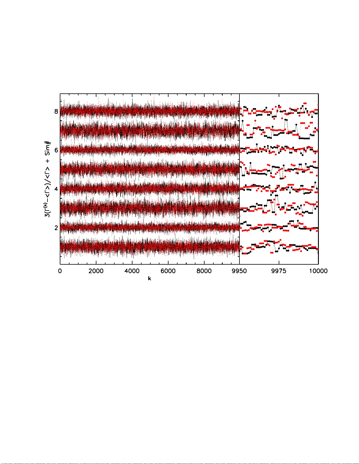
Accoun ting for Calibration Uncertain t ies in X-r a y A nalysis: Eﬀectiv e Areas in Sp ectral F itting Hyunso o k Lee 1 , Vina y L. Kash y ap 1 , Da vid A. v an Dyk 2 , Alanna Connors 3 , Jerem y J. Drake 1 , Rima Izem 4 , Xiao- Li Meng 5 , Shandong Min 2 , T aey oung P a r k 6 , P ete Rat zlaﬀ 1 , Aneta Siemigino wsk a 1 , and Andreas Zezas 7 , 8 1 Smithsonian Astroph ysical Observ a t o ry , 60 Garden Street, Cambridge, MA 02138 hlee@cfa.ha rvard.edu vkashyap@cf a.harvard.ed u jdrake@cfa. harvard.edu rpete@head. cfa.harvard. edu asiemiginow ska@cfa.harv ard.edu 2 Departmen t of Statistics, Univ ersit y of California, Irvine, CA 926 97-1250 dvd@ics.uci .edu shandonm@uc i.edu 3 Eurek a Scientiﬁc , 2 452 Delmer Street Suite 100, O akland CA 9460 2-3017 aconnors@eu rekabayes.co m 4 US F o o d and D rug Administration, Cen ter for Drug Ev aluatio n and Research , Division of Biometrics 4, 10903 New Hampshire Av e, Silv er spring, MD 2 0903 rima.izem@f da.hhs.gov 5 Departmen t of Statistics, Harv ard Univ ersit y , 1 Oxford Street, Cambridge, MA 02138 meng@stat.h arvard.edu 6 Departmen t of Applied Statistics, Y onsei Univ ersity , Seoul 120-74 9, South K orea taeyoung.t. park@gmail.c om 7 IESL, F oundation for R esearc h and T ec hnology , 711 10, Heraklion, Crete, G reece – 2 – 8 Ph ysics D epartmen t, Univ ersit y of Crete, P .O. Bo x 2 208, 710 03, Heraklion, Crete, Greece azezas@phys ics.uoc.edu Receiv ed ; accepted accepted for publication in ApJ – 3 – ABSTRACT While considerable adv ance has b een made to a ccount for statistical un- certain t ies in astronomical analyses, systematic instrumen tal uncertain ties hav e b een gene rally ignored. T his can b e crucial to a prop er interpretation of analysis results b ecause instrumen ta l calibration uncertaint y is a for m of systematic un- certain ty . Ignoring it can underestimate error bars and introduce bias in to the ﬁtted v alues of mo del parameters. Accoun ting for suc h uncertain ties currently requires extensiv e case-sp eciﬁc sim ula t io ns if using existing analysis pack ages. Here w e presen t general statistical metho ds that incorp o rate calibration uncer- tain ties into sp ectral analysis of high-energy data. W e ﬁrst presen t a metho d based o n m ultiple imputation that can b e a pplied with an y ﬁtting metho d, but is necessarily approx imate. W e then describ e a mor e exact Ba y esian approach that w orks in conjunction with a Mark o v chain Mon te Carlo based ﬁtting. W e explore metho ds for improving computational eﬃciency , and in particular detail a metho d of summarizing calibration uncertain ties with a principal comp onen t analysis of samples of plausible calibration ﬁles. T his method is implemen ted using recen tly co diﬁed Chandra eﬀectiv e area uncertain ties for lo w-resolution sp ectral analysis and is v eriﬁed using b oth sim ulated and actual Chandra data. Our pro cedure for incorp orating eﬀectiv e area uncertain t y is easily generalized to o t her types of calibration uncertain ties. Subje ct he adings: X-ra ys: general, m etho d s: data analysis, metho ds: statistic al, tec hn iques: miscellaneous – 4 – 1. In tro duction The imp o rtance of accoun ting for statistical errors is w ell established in a stro no mical analysis: a measuremen t is of little v alue without a n estimate of its credible range. V arious strategies hav e b een dev elop ed to compute uncertain ties resulting from the con volution of photon coun t data with instrume n t calibration pro ducts suc h as eﬀec tiv e area curv es, energy redistribution matrices, and p oint spread functions. A ma jor comp onent of these a na lyses is go o d kno wledge o f the instrumen t characteristic s, describ ed by the instrumen t calibration data. Without the transformation from measuremen t signals to ph ysically in teresting units aﬀorded by the instrumen t calibration, the observ ational results canno t b e understo o d in a meaningful wa y . How ev er, ev en tho ug h it is w ell kno wn that the measuremen ts of the instrumen t’s prop erties (e.g., quan tum eﬃciency of a CCD detector, p oin t spread function of a telescop e, etc.) hav e asso ciated measuremen t uncertain ties, the calibration of instrumen ts is often taken on faith, with only nominal estimates used in data analysis, ev en when it is recognized that these uncertain ties can cause large systematic errors in the inferred mo del parameters. 1 In many subﬁelds (exceptions include: e.g. gravitational w a v e 1 Ho w ev er in ground-based observ ations, it is customary to describe non-instrumen tal systematics as calibration uncertaint y , especially time-v ariable and fo reground eﬀects, and incorp orate them in the ﬁnal uncertainties . These include: e.g. atmospheric absorption eﬀects on photometry , ﬂat-ﬁelding, and a stro metric calibration, as in T aris et al. 2011, Aguirre et al. 2011; calibrating brightne ss of distan t ob jects in the presence of foregro und dust (Conley et al 2011, Kim and Miquel 20 0 6, Mandel et al. 2009). As w ell, uncertain ties asso ciated with the basic ph ysics, such as e.g. sp eciﬁc stellar absorption lines (Thomas, Maraston, and Johansson 2010) ; or other mo del-mismatc h uncertain ties, suc h as intrinsic SN ligh t-curv e v ariat io ns (Conley et al 2011, Kim and Miquel 2006, Mandel et al. 2009), can also b e referred to as calibration uncertain ties in the literat ur e. In this pap er, w e sp eciﬁcally – 5 – astroph ysics, VIR G O Collab oration 2010, LIGO Collab oration 2010 a nd references therein; CMB ana lyses, Mather et a l. 1999, Rosset et al. 20 10, Jarosik et al. 201 1, and references therein; a nd extra-solar planet/planetary disk w ork, e.g. Butler et al. 1996, Maness et al. 2011, and references therein), instrumen t calibration uncertain ty is often ignored en tirely , or in some cases, it is assumed that the calibration error is uniform across an energy band or a n image area. This can lead to erroneous in terpretation of the da t a. Calibration pro ducts are deriv ed b y comparing data from w ell-deﬁned sources obtained in strictly con t r o lled conditio ns with predictions, either in the lab or using a particularly w ell-understo o d astroph ysical source. P arametrized mo dels are ﬁt to these data to deriv e b est-ﬁt parameters that are then used to derive the relev an t calibration pro ducts. T he errors on these b est-ﬁt v alues carry information o n how a ccurately the calibration is kno wn and could b e used to accoun t for calibration uncertain ty in mo del ﬁtting. Unfortunately , ho w ev er, the errors on the ﬁtted v alues are routinely discarded. Ev en b ey ond the errors in these ﬁtted v alues, calibration pro ducts are sub ject to uncertaint y stemming from diﬀerences b et w een the idealized calibration experiments and the m yriad of complex settings in whic h the pro ducts ar e used. Susp ected system atic uncertain t y cannot b e fully understo o d until suitable data are acquired or cross-instrumen t comparisons are made (Dav id et al. 200 7 ). Prosp ectiv ely , this source of uncertain ty is diﬃcult to quan tify but is encompassed to a certain exten t in the exp erience of the calibration scien tists. Diﬀeren t mec hanisms ha v e b een prop osed to quan tify this type of uncertaint y , ra nging f r om ado pting ad ho c distributions suc h as truncated Gaussian (D rak e et al. 200 6 ) to uniform deviations o v er a sp eciﬁed range. As long as it can b e c haracterized ev en lo o sely , statistical theory pro vides a mec hanism by which this informatio n can b e included to b etter estimate the concen trate o n instrumen tal calibration uncertain ties, although the formalisms intro duced could in principle handle other kinds of systematic errors. – 6 – errors in the ﬁnal analysis. Users and instrumen t builders agr ee that incorp orating calibration uncertain t y is imp ortant (see Davis 2001; Dr a k e et al. 2006; Grimm et al. 20 09). F or example, Drak e et al. (2006) demonstrated that error bars on sp ectral mo del parameters are underestimated b y as m uch as a factor of 5 (see their Figure 5) for high coun ts data when calibration uncertaint y is ignored ( >> 10 3 coun t s for t ypical CCD resolution sp ectra). Suc h underestimations can lead to incorrect interpretations of the analysis results. Despite this, calibration uncertain ties a re rarely incorp ora ted b ecause only a few ad ho c tec hniques exist and no robust principled metho d is av ailable. In short, there is no common language or standard pro cedure to accoun t for calibration uncertain t y . Historically , at the In ternational Congress of Radiolog y and Electricit y held in Brussels in Septem b er 1910, MMe. Curie was ask ed to prepare the ﬁrst standard based on high energy photon emission (X-/ γ -ray ): 21.99 milligra ms of pure radium c hloride in a sealed glass tube, equiv alen t to 1.67x10 − 2 Curies of radioactiv e radium (e.g., Brown 1997 pg 9ﬀ and references therein). The problem then b ecame: ho w to measure other samples, in reference to t his standard? Although the sample preparation w as do ne by v ery accurate c hemistry tec hniques, the tric ky part w a s designing and building the instrumen t to quan tify the high-energy photon emission. At the next In ternational Committee meeting (1912, P aris) calibrating the standard w as done by sp ecialized electroscop es ba lancing the ‘ionization curren t’ from tw o sources. This instrumen t w as deemed to ha v e an uncertain t y of one part in 400 (Rutherford and Chadwic k 1 911). The original pap er also describ es a metho d for calibrating the detector. Although these measuremen ts w ere quite carefully done, and complex fo r their time, the result w as a single v alue (the intensit y) and had a single n umber quan tif ying its error ( 1 400 ; Rutherford a nd Chadwic k 191 1 ). In this case, the eﬀect of t his original una v o ida ble measuremen t error on one’s ﬁnal measuremen t of a source in tensity (in – 7 – Curies) is straightforw ard to propagate, suc h as by the delta-metho d. No w adays, meetings a b out absolute standards and measuring instruments are m uc h more complex, incorp orating m ultiple kinds of measuremen ts for a single standard (e.g. COD A T A; Mohr, T aylor, and New ell 2008). As w ell, in the general literature, one ﬁnds increasingly complex metho ds dealing with e.g. multiv ar iate data and calibra tion (Sundb erg 1999, Osb ourne 19 9 1), and ev en metho ds f or ‘t r a ceabilit y’ bac k to kno wn standards ( Cox and Harris 2006). Thes e approac hes for m ulat e their complexities in terms of cross-correlations of parameters. This metho dology has also b een successfully used in mo dern astroph ysics, such as in combining optical observ ations of sup ernov ae for cosmological purp oses (e.g. Kim and Miquel 2006). Initially , J. D rak e and ot her co-authors did try for mulating the dep endencies and anticorrelations of the ﬁnal calibration pro duct uncertain ties in t erms of correlation co eﬃcien ts. Ho w ev er, after considerable exploration, they found this a ppro ac h unable to capture the complexities of spacecraft calibration, esp ecially at high energies. F irst, each part o f a mo dern instrumen t suc h as the Chandra observ a tory is measured a t multiple energies and m ultiple p ositions, a s we ll as calibrat ing the whole system on the ground. Second, in terestingly , the instrumen t is mo deled by a complex ph ysics-base d computer co de. The original calibration measuremen ts are not used directly , but are b enc hmarks fo r the phy sical systems mo deled therein. High energy astroph ysics brings a third diﬃcult y: the previous pap ers assumed a Ga uss-Normal distribution for the calibration-pro duct uncertain ties; this certainly do es not hold for most real instrumen ts in the high energy regime. Hence, expanding b ey ond Drake et al. (2006), in this pa p er, w e describ e how to ‘short-circuit’ tra cing back to the original calibration uncertain t ies b y using the en tire instrumen t-mo deling co de as part of statistical computing tec hniques. W e see this in the con text of the mov emen t tow ards “uncertain t y quan tiﬁcatio n” (UQ) of larg e computer co des (see, e.g., Christie et al. 2005). – 8 – Un t il recen t ly , the b est av ailable general strategy in high-energy astroph ysics w as to compute the ro o t - mean-square o f the measuremen t erro rs a nd the calibration errors and then to ﬁt the source mo del using the resulting error sum (see Bevington and Robinson 1992). Unfortunately , the use and interpretation of the standard deviation relies on Gaussian errors, that the calibration errors are uncorrelated, and that the uncertaint y on the calibration pro ducts can b e uniquely tr anslated t o an uncertain t y in each bin in da ta space. None of these assumptions are w arra nted. F urthermore, this metho d, equiv alen t to artiﬁcially inﬂating the stat istical uncertain ty on the data, will lead to biased ﬁts, error bars without prop er co verage, a nd incorrect estimates o f go o dness o f ﬁt. Individual g roups hav e also tried v arious instrumen t-sp eciﬁc metho ds. These range from b o otstrapping (Simpson and Ma yer-Hasse lw a nder 1986) to raising and lo w ering resp onse “wings” b y hand (F Orrest 1988, F orrest V estrand and McConnell 1997), and in one case, analytical marginalizat io n o v er a particular kind of instrumen tal uncertain t y ( Br idle et al. 200 2). I n general a nd in imp o rtan t cro ss-instrumen t comparisons, how ev er, all but the crudest metho ds (e.g., m ultiplying eac h instrumen t’s total eﬀectiv e area b y a ﬁtted “uncertain t y fa cto r ” a s in Hanlon et al. 1995, Sc hmelz et al. 200 9) are v ery diﬃcult to handle. Metho ds for ha ndling systematic erro r s exist in o t her ﬁelds suc h a s particle phys ics (Heinric h and Lyons 2 007 and references therein) and o bserv ational cosmology ( Br idle et al. 20 0 2). I n their review of systematic errors, Heinric h and Ly o ns (2007) a dv o cate parameterizing the systematics in to statistical mo dels and marginalizing ov er the n uisance parameters of the systematics . They described v arious statistical strategies to incorp orate systematic errors whic h range from simple brute force χ 2 ﬁtting to fully Bay esian hierarchical mo deling. Unfortunately these analytical metho ds rely on G aussian mo del assumption that are inappropriate for high energy astroph ysics and are also highly case sp eciﬁc. Accoun ting for calibration uncertain t y is further complicated b y complex and la rge – 9 – scale correlation in the calibratio n pro ducts. Th e v alue of the calibration pro duct at o ne p oin t can dep end strongly on far aw a y v alues and even data collected using a diﬀerent instrumen t. F or example, the Chandra Low Energy T ransmission Grating Sp ectrometer (LETGS) + High Resolution Camera - Sp ectroscopic readout (HR C-S) eﬀectiv e area is calibrated using the p o w er-la w source PKS 2 155-304. Because the high-or der contributions to the sp ectrum cannot b e disen tangled, the index of the p ow er-la w dep ends strongly on an analysis of the same source with data obtained contempora neously with the High Energy T ransmission G r ating Sp ectrometer (HETGS) + ACIS-S. Th us, changes in the HETGS+A CIS-S eﬀectiv e area will aﬀect the longer-w a v elength LETGS+HR C-S eﬀectiv e area. The complex correlations can result in a div erse set of plausible eﬀectiv e a rea curv es. The c hoice among these curv es can strongly aﬀect the ﬁnal b est ﬁt in day-to-da y a nalyses. The nominally b etter strategy of folding the calibrat ion uncertain ty through to the ﬁnal statistical errors on ﬁtted mo del par a meters is unfortuna t ely unfeasible: the complex correlations mak e it diﬃcult to quan tify the aﬀect on the ﬁna l analysis of uncertaint y in the calibration pro duct. Drak e et al. (2006) pro p osed a strategy that accounts for these correlations b y generating syn thetic dat a sets from a nominal eﬀectiv e area and then ﬁtting a mo del separately using each of a num b er of instance of a simulated eﬀectiv e area and then estimating the eﬀect of the calibration erro r via the v ariance in the resulting ﬁtted mo del parameters. Th is pro cedure can b e implemen ted using standard softw are pac k ages suc h as XSPEC (Arnaud 1 996) and Sherp a (F reeman et al. 2001, Refsdal et al. 200 9 ) and demonstrates the imp ortance of including calibration errors in data ana lysis. Ho w ev er, in practice there are some diﬃculties in implemen ting it with real data where the true parameters a re not known a prio ri . The ad ho c nature of t he b o o tstrapping-t yp e pro cedure means its statistical pro p erties are no t w ell understo o d, requiring t he sampling distributions to b e calibrated on a case-b y-case basis. That is, the pro cedure requires v eriﬁcation – 10 – whenev er diﬀeren t mo dels are considered or diﬀerent pa rts of the pa rameter space are explored. The large nu m b er of ﬁts required also imp oses a heavy computational cost. Most imp ortantly , it requires n umerous sim ulated calibration pro ducts that m ust b e supplied to end users either directly through a comprehensiv e databa se or through instrumen t sp eciﬁc soft w are fo r generating them. In general, b oth these strategies imp o se a heavy burden on calibration or a nalysis sof tw are main tainers. The primary o b jectiv e of this article is to prop ose well-deﬁn ed and general metho ds to incorp orate complex calibration uncertain ty in to sp ectral analysis in a manner that can b e replicated in general practice without precise calibration exp ertise. Although we dev elop a general framew ork fo r incorp orat ing calibra tion uncertain t y , we limit our detailed discussion to a ccounting for uncertain t y in the eﬀectiv e area for Chandra /A CIS-S in sp ectral analysis. W e prop ose a Ba ye sian f ramew ork, where kno wledge of calibration uncertain ties is quan tiﬁed through a prior probabilit y . In this w ay , information quantiﬁe d b y calibration scien tists can b e incorp orated into a coherent statistical analysis. Op erationally , this in v olv es ﬁtting a highly-structured statistical mo del that do es not assume the calibra tion pro ducts ar e kno wn ﬁxed quan tities, but rather incorp o rates their uncertain ty through a prior distribution. W e describe t w o statistical strat egies b elow for incorp or ating this uncertaint y in to the ﬁnal ﬁt. Multiple imputation ﬁts the mo del sev eral times using standard ﬁtting routines, but with a diﬀeren t v alue of the calibration pro duct used in eac h ﬁt. Alternativ ely , using an iterativ e Mark o v ch ain Monte Carlo (MCMC) sampler allow s us to incorp o rate calibration uncertain ty directly in to the ﬁtting routine b y up dating the calibration pro ducts a t each iteration. In either case, we adv o cate up dating the calibration pro ducts based solely on information pro vided b y calibration scien tists and not on the data b eing analyzed (i.e., not up dating pro ducts giv en the data b eing analyzed; see also discuss ion ab out computational feasibilit y in § 6 .1). This strategy leads to simpliﬁed computation and reliance on t he exp ertise of the calibratio n scien tists rather tha n on the idiosyncratic f eatures of the data. – 11 – W e adopt the strategy o f Dra ke et al. (2006) to quantify calibration uncertain t y using an ensem ble of sim ulated calibration pro ducts, that w e call the calibration sample . W e use Principal Comp onent Analysis ( PCA) to simplify this represen tatio n. A glossary o f the terms and sym b ols tha t w e use is giv en in T able 1. In § 2 w e describe the calibration sample and illustrate the imp orta nce of prop erly accoun ting for calibra tion uncertain t y in sp ectral analysis. Our basic metho dology is outlined in § 3, where w e describe how the calibration sampler can b e used to generate the replicates necessary for m ultiple imputation or can b e incorp orated into an MCMC ﬁtting a lg orithm. W e also sho w ho w PCA can provide a concise summary of the complex correlations of the calibration uncertain t y . Speciﬁc algo rithms a nd strategies for implemen ting this g eneral framew o rk for sp ectral analysis app ear in § 4. Our pro p osed metho ds are illustrated with a simu lation study and an analysis of 15 radio loud quasars (Siemigino wsk a et al. 2008) in § 5. In § 6 w e discuss future dir ections and a g eneral framework for handling calibra tion uncertain ties from astroph ysical observ ations with similar form as our yX-ray examples . W e summarize the w ork in § 7. 2. The Calibration Sample and t he Eﬀect of Calibration Uncertaint y T o coheren tly and con venie n tly incorp ora te calibration uncertaint y in to sp ectral ﬁtting, w e follow t he suggestion of D rak e et al. (2006) to represen t it using a randomly generated set of calibratio n pro ducts that we call the calibration sample . In this section we b egin b y describing this calibration sample, and how it can b e used t o represen t the inheren t systematic uncertain ty . The metho ds that w e discuss in this and the follow ing sections are quite general and in principle can b e applied to accoun t fo r system atic uncertaint y in any calibration pro duct. F or clarity , w e illustrate their application to instrumen t eﬀectiv e areas. – 12 – 2.1. Represen t ing Uncertaint y W e b egin with a simple mo del of telescope resp onse that assumes p osition and time in v ariance. In particular, supp ose the resp onse of a detector to an inciden t photon sp ectrum S ( E ; θ ), M ( E ∗ ; θ ) = X E S ( E ; θ ) A ( E ) P ( E ) R ( E ∗ ; E ) , (1) where E ∗ represen ts the detector c hannel at which a phot o n of energy E is recorded, θ represen ts the parameters of the source mo del, and A , P , a nd R are the eﬀectiv e area, p oin t spread function, and energy redistribution matrix of the detector, resp ectiv ely . W e aim to dev elop metho ds t o estimate θ and compute error bars that pro p erly accoun t for uncertain ty in A . Of course P and R are also sub ject to uncertain t y and in § 6.2 we discuss extensions of the metho ds described here to handle more general sources of calibratio n uncertain ty . As an illustration, we consider observ ations obtained using the spectroscopic array of the Chandra AXAF CCD Imaging Sp ectrometer detector (AC IS-S). According to Drake et al. (2006), it is p ossible to generate a calibration sample of eﬀectiv e area curve s fo r this instrumen t b y explicitly including uncertainties in each of its subsystems (UV/Ion shield transmittance, CCD Quantum Eﬃciency , and the telescop e mirror reﬂectivit y). The result is a set of sim ulatio ns of the eﬀectiv e area curv es. These encompass the range of its uncertain t y , with more of the sim ula t ed curv es similar to its most lik ely v alue, and few er curv es that r epresen t p ossible but less likely v alues. In principle, some ma y b e more lik ely than others, in whic h case weigh ts that indicate the relat ive lik eliho o d are required. In this article, w e assume that all of the sim ulations in the set are equally lik ely , that is the sim ulations are represen tativ e of calibration uncertaint y . The set of L simu lations is the calibration sample and denoted A = { A 1 , . . . , A L } , where A l is one of the sim ulated eﬀectiv e area curv es. – 13 – The complicated structure in the uncertaint y for the true eﬀectiv e a r ea is illustrated in Figure 1 using the calibra tion sample of size L = 1000 generated b y Drak e et al. (2006). A selection of six of the A l from A are plotted a s colored dashed lines and compared with the default eﬀectiv e ar ea, A 0 that is plotted as a solid black line. The second panel plo ts t he diﬀerences, A l − A 0 for the same selection. The light gray area represen ts the full range of A and the dark gray area represen t s interv als that con tain 68.3% of the A l at eac h energy . The complexity of the uncertaint y of A is eviden t. W e use the calibration sample illustrated in Figure 1 as the represen tativ e example througho ut this article. 2.2. The Eﬀect of the Uncertaint y W e discuss here the eﬀect of the uncertain ty represen ted by the calibratio n sample on ﬁtted sp ectral parameters and their error bars. W e employ sim ula ted sp ectra represen t ing a broad range in parameter v alues. In particular, we simu lated four data sets of an absorb ed p o w er-la w source with three para meters (p ow er-la w index Γ, absorption column densit y N H , and normalization) using the fakeit routine in XSPECv12 . The data sets we re all sim ulated without background con tamination using the XSPEC mo del wabs*powerlaw , nominal default eﬀectiv e area A 0 from the calibration sample of Drak e et a l. (20 06), and a default RMF fo r A CIS-S. The p ow er la w pa rameter (Γ), column densit y ( N H ), and nominal counts for the four simulations (see also T able 2) w ere Simula tion 1 : Γ = 2 , N H = 10 23 cm − 2 , and 1 0 5 coun t s; Simula tion 2 : Γ = 1 , N H = 10 21 cm − 2 , and 1 0 5 coun t s; Simula tion 3 : Γ = 2 , N H = 10 23 cm − 2 , and 1 0 4 coun t s; and Simula tion 4 : Γ = 1 , N H = 10 21 cm − 2 , and 1 0 4 coun t s – 14 – resp ectiv ely . T o illustrate the eﬀect of calibration uncertain ty , w e selected the 1 5 curv es in A l ∈ A with the largest maxim um v alues and the 15 curves with the smallest maxim um v alues. In some sense, these are the 30 most extreme eﬀectiv e area curv es in A . They are plotted as A l − A 0 in the ﬁrst panel o f Figure 2, alo ng with a horizontal line at zero that represen ts the default ( A 0 − A 0 ). W e used the Ba y esian metho d of v an Dyk et al. (2001) to ﬁt Simula tion 1 and Simula tion 2 eac h 31 times, using eac h of the 31 curv es of A l plotted in Figure 2. The resulting marginal and j oin t p osterior distributions for Γ and N H app ear in row s 2 -4 of F ig ure 2; the con tours plotted in the third r ow corresp o nd to a p osterior probabilit y of 9 5 % for each ﬁt. 2 The ﬁgure clearly shows that the eﬀect of calibra t io n uncertain ty sw amps the ordinary statistical error. The scien tist who assumes that the true eﬀectiv e area is known to b e A 0 ma y dra matically underestimate the erro r bars, and may miss the correct region en tirely . As a second illustration w e ﬁt Simula tion 1 and Simula tion 3 eac h 31 times, using the same A l as in F igure 2 and with A 0 , again using the metho d of v an Dyk et al. ( 2 001). The resulting p osterior distributions of Γ and N H are plotted in Figure 3. Comparing the t w o columns o f the ﬁgure, the relativ e contribution of calibratio n uncertain t y to the total error bars app ears to gro w with coun ts. F or this reason, accoun ting for calibration uncertain ty is esp ecially imp or t an t with ric h high-coun t sp ectra. In fact, in our sim ulations there app ears to b e a limiting v alue where the statistical errors are negligible and the total 2 The con tours in Figure 2 w ere constructed b y p eeling (Gr een 1980) the original Monte Carlo sample. This in volv es remo ving the most extreme sampled v alues whic h are deﬁned a s the v ertices of the smallest conv ex set con taining the sample ( i.e., the con v ex h ull). This is rep eated un til only 95% of the sample remains. The ﬁnal h ull is plotted as the con tour. This is a reasonable approximation b ecause the p osterior distributions app ear roughly conv ex. – 15 – error bars are due en tir ely to calibration uncertain t y . The total error bars do not go b elo w this limiting v alue regardless of ho w man y coun ts are observ ed. W e mus t emphasize, how ev er, that we ar e assuming t hat the observ ed coun ts a re uninformativ e as to whic h of the calibration pro ducts in the calibra t ion sample are more or less lik ely . If w e w ere no t to mak e t his assumption, how ev er, and if a data set we re so large that w e w ere able to exclude a large p ortion of the calibration sample as inconsisten t with the data, the remaining calibration uncertain ty w ould b e reduced and its eﬀect w ould b e mitigated. In this case, the default eﬀectiv e area and eﬀectiv e area curv es similar to the default could p oten t ially b e found inconsisten t with the data and thu s the ﬁtted mo del parameters could b e diﬀeren t from what w e would get if we simply relied on the default curv e. In this ar t icle, ho w ev er, w e assume that either the data set is not large enough to b e informative for the calibration pro ducts or that w e do not wish to base instrumen tal calibration on the idiosyncrasies of a particular data set. Both Figures 2 and 3 suggest that while the ﬁtted v alues dep end on the choice of A ∈ A , the statistical erro rs for the parameters giv en an y ﬁxed A ∈ A are more-o r - less constan t. The systematic errors due to calibration uncertain t y shift the ﬁtted v alue but do not eﬀect its v ariance. Of course, in practice w e do not kno w A and m ust marginalize ov er it, so the total error bars are larger than any of the errors bars that a r e computed giv en a particular ﬁxed A . How to coheren tly compute error bars that a ccount for calibration uncertain ty is o ur next topic. 3. Sp ectral Analysis Using a Calibration Sample of the Eﬀective Ar ea In this section, we outline how the calibration sample can b e used in principled statistical analyses and describe how the complex calibration sample can b e summarized in – 16 – a concise and complete manner using PCA. 3.1. Statistical A nalysis wit h a C alibration Sample 3.1.1. Mar ginalizing over Calibr ation Unc ertainty In a standard astronomical data analysis problem, as represen ted by Equation 1, it is assumed that A ≡ A 0 and that θ is estimated using p ( θ | Y , A 0 ), where Y is the observ ed coun t s and p is an ob jectiv e function used for probabilistic estimation and calculation of error bars. Ty pical c hoices of p are the Ba y esian p osterior distribution, t he lik eliho o d function, the Cash statistic, or a χ 2 statistic. W e use the notation p ( θ | Y , A 0 ) b ecause w e generally tak e a Ba y esian p ersp ectiv e, with p ( · ) represen ting a probability distribution and the notatio n “ | ” referring to conditioning, e.g., p ( U | V ) is to b e read as “the probabilit y of U g iv en tha t V is true.” When A is unkno wn, it b ecomes a nuisance parameter 3 in the mo del, and the appropriate ob jectiv e function b ecomes p (mo del parameters , A | data). Using Ba y esian notation, p ( θ , A | Y , Z ) = p ( θ | Y , Z , A ) p ( A | Y , Z ) , where the primary source of infor mation for A is not the observ ation counts , Y , but the large datasets and ph ysical calcuations used by calibratio n scien tists, and whic h we denote here b y Z . Generally sp eaking, we exp ect the information for θ to come from Y rather than Z , at least giv en A and w e exp ect the information for A to come from Z rather than Y . 3 A nuisanc e para meter is simply an unkno wn but necessary parameter in the mo del that is not of direct in terest. Its presence in the mo del ma y complicate inference, whic h can b e a n uisance. – 17 – This can b e expressed mathematically by t w o conditional indep endence assumptions: 1. p ( θ | Y , Z , A ) = p ( θ | Y , A ), and 2. p ( A | Y , Z ) = p ( A | Z ). W e mak e these conditional indep endence assumptions, and implicitly condition on Z throughout this article. In this case, w e can rewrite the ab o v e equation as p ( θ , A | Y ) = p ( θ | Y , A ) p ( A ) , (2) whic h eﬀectiv ely replaces the p o sterior distribution p ( A | Y ) with the prior distribution p ( A ). Finally , w e can fo cus atten tion on θ by marginalizing out A , p ( θ | Y ) ≈ Z p ( θ | Y , A ) p ( A ) d A ≈ 1 L L X l =1 p ( θ | Y , A l ) . (3) That is, the o b jectiv e function is simply the av erage o f the ob jectiv e functions used in t he standard analysis, but with A 0 replaced by each of the A l ∈ A . Th us, the mar g inalization in Equation 2 do es not necessarily inv olv e estimating p ( A | Y ) nor sp ecifying a parametric prior or p osterior distributions for A . When this margina lizat io n is prop erly computed, systematic errors from calibratio n uncertain t y are rigoro usly com bined with statistical errors without need for Gaussian quadrature. Of course, when L is la r g e as in the calibration sample of Drak e et al. (200 6), ev aluating and optimizing Equation 3 w ould b e a computationally expensiv e task. In this section w e outline tw o strategies that aim to signiﬁcan tly simplify the necessary computation. The ﬁrst is a general purp ose but approximate strategy that can b e used with any standard mo del ﬁtting techniq ue and the second is a simple a daptation that can b e emplo y ed when Mon t e Carlo is used in Ba y esian mo del ﬁtting. Details and illustrations o f b oth metho ds app ear in § 4. – 18 – 3.1.2. Multiple Im p utation The ﬁrst strategy tak es adv an tage of a well-es tablished statistical tec hnique kno wn as m ultiple imputation that is designed to handle missing data (Rubin 1987, Schafer 1 9 97). Multiple Imputation relies on the a v ailabilit y o f a n um b er of Monte Carlo replications of the missing data. The replications are called the imputations and are designed to represen t the statistical uncertain ty regarding the unobserv ed v alues of the missing da t a. Although the calibration pro ducts are not missing data p er se , the calibration sample prov ides exactly what is needed for us to apply t he metho d of m ultiple imputation: a Mon te Carlo sample that represen ts the uncertain t y in an uno bserv ed quantit y . With the calibration sample in hand, it is straightforw ard to apply m ultiple imputation. A subset of A of size M ≪ L is randomly selected and called the m ultiple imputat ions or the m ultiple imputation sample . The standard data analysis metho d is then applied M times, once with eac h of the M imputations of the calibratio n pro ducts. This pro duces M sets of parameter estimates along with their estimated v ariance-cov ariance matrices 4 , whic h w e denote ˆ θ m and V a r( ˆ θ m ), resp ectiv ely , fo r m = 1 , . . . , M . In the simplest form of the metho d of m ultiple imputation, we assume that eac h ˆ θ m follo ws a m ultiv ariate normal distribution with mean θ . The ﬁnal ﬁtted v alues and error bars are computed using a set of simple momen t calculations know n as the m ultiple imputation com bining rules (e.g., Harel and Zhou 2005). The para meter estimate is computed simply as the a v erage of the individual ﬁtted v alues, ˆ θ = 1 M M X m =1 ˆ θ m . (4) 4 The v aria nce-co v aria nce matrix is a matrix that has the square of the error bars along its diagona l and the cov ariance terms as oﬀ- diagnonal elemen ts. Recall that the cov ar ia nce is the correlation times the pro duct of t he error bars: Co v ( X , Y ) = Correlation( X , Y ) σ x σ Y . – 19 – T o compute the erro r bars, we m ust combine t w o sources of uncertaint y: the statistical uncertain ty that would a rise ev en if the calibration pro duct were know n with certain t y and the systematic uncertaint y stemming from uncertaint y in the calibration pro duct. Eac h of the M standard a nalyses is computed as if t he calibration pro duct we re known and therefore eac h V ar( ˆ θ m ) is an estimate of the statistical uncertaint y . Our estimate of the statistical uncertain ty is simply the a v erag e of these individual estimates, W = 1 M M X m =1 V ar( ˆ θ m ) . (5) The systematic uncertain t y , on the other hand, is estimated by lo o king at ho w c ha nging the calibration pro duct in eac h of the M analyses aﬀects the ﬁtted parameter. Th us, the systematic uncertain ty is estimated as the v ariance of the ﬁtted v alues, B = 1 M − 1 M X m =1 ( ˆ θ m − ˆ θ )( ˆ θ m − ˆ θ ) ⊤ . (6) Finally the tw o comp onen ts of v ariance are combin ed for the t o tal uncertaint y , T = W +  1 + 1 M  B , (7) where the 1 M term accounts for small n um b er M of imputations. If M is small relative to the dimension of θ , T will b e unstable, and more sophisticated estimates should b e used (e.g., Li et al. 1991) . Here w e fo cus on univ ariate summaries and error bars whic h dep end only on o ne elemen t of ˆ θ and the corresp onding diagonal elemen t o f T . When computing the error bars for one of the univ ariate ﬁtted parameters in ˆ θ , sa y comp onen t m of ˆ θ , it is generally recommended that the n um b er of sigma used b e inﬂated to a dj ust for the t ypically small v alue of M . That is, rather than using one- and tw o-sigma for 6 8.3% and 95.4 % in terv als a s is appropriate for t he norma l distribution, a t distribution should b e used, requiring a larger n um b er of sigma to obtain 68.3% and 95.4% in terv als. In the univ ariate case, t he degrees of freedom of the t distribution determine the degree of – 20 – inﬂation and can b e estimated b y degrees of freedom = ( M − 1)  1 + M W mm ( M + 1) B mm  2 , (8) where W mm and B mm are the m th diagonal terms of W and B . The metho d of multiple imputation is based on a n um b er of assumptions. First, it is designed t o g iv e a ppro ximate error bars o n θ that include the eﬀects of the imputed quan tity , but if a full p osterior distribution on θ is desired, then a more detailed Ba yes ian calculation must b e p erformed (see b elo w). It will pro vide a n approximately v alid answ er in general when the imputation mo del is compatible with t he estimation pro cedure, i.e., when ˆ θ is the p osterior mo de from essen tia lly the same distribution as is used f or the imputation (Meng 1994). F urthermore, the computed standard deviations √ T can b e iden tiﬁed with 68% credible in terv als only when the p osterior distributions are multi-v ariate Normal. Additionally , when M is small, the cov erage must b e adjusted using the t -distribution (Equation 8). 3.1.3. Monte Carlo in a Bayesian Statistic al Analysis Multiple imputation oﬀers a simple g eneral strategy for accoun ting for calibration uncertain ty using standard a nalysis metho ds. Because this metho d is only approximate, ho w ev er, our preferred solution is a Mon te Carlo metho d that is ro bust, reliable, a nd fast. In principle, Mon te Carlo metho ds can handle any lev el of complexit y presen t in b oth the astrophys ical mo dels a nd in t he calibration uncertain ty . Mon te Carlo can b e used to construct p ow erful metho ds that are a ble to explore interes ting regions in high-dimensional par a meter spaces and, for instance, determine b est-ﬁt v alues of mo del parameters along with their erro r bars. In this con text, it is used as a ﬁtting engine, similar to Lev enberg-Marquardt, Po w ell, Simplex, and ot her minimization alg o rithms. One of – 21 – its main adv antages is that it is highly ﬂexible a nd can b e applied to a wide v ariet y of problems. A single run is suﬃcien t to describ e the v aria t ions in t he mo del parameters that arise due to b oth statistical and systematic errors, which therefore leads to reduced computational costs. 5 Consider a Mon te Carlo sample obtained by sampling the mo del parameters θ give n the data, Y , and the calibration pro duct, A = A 0 , θ ( k ) ∼ p ( θ | Y , A 0 ) , where k is the itera t io n n umber and θ ( k ) are the v alues of the para meters at iteration k . The set o f para meter v alues th us obtained is used to estimate t he b est-ﬁt v alues and the error bars. When calibration uncertain t y is included, w e can no longer condition on A 0 as a kno wn v alue of the calibratio n pro duct. Instead w e add a new step that up da t es A according t o the calibrat io n uncertainties . In part icular, θ ( k ) is up dat ed using the same iterativ e algorithm as ab ov e, with an additional step at each iteration that up dates A . Supp ose at iteration k , A ( k ) is the r ealizat io n of t he calibratio n pro duct. Then the new algorithm consists of the following t w o steps: A ( k ) is sampled fro m p ( A | Y ) and θ ( k ) is sampled fro m p ( θ | Y , A ( k ) ) . Under the conditional indep endence assumptions of Section 3.1.1, w e can simplify this sampler b y replacing p ( A | Y ) with p ( A ) in the ﬁrst step: A ( k ) is sampled fro m p ( A ) and (9) 5 In most cases, Mark o v chain Mon te Carlo (MCMC) rather tha n simple Monte Carlo is required to explore complicated pa r a meter spaces. Unfortunately , the use of MCMC in this situation r a ises certain techn ical complications. In this section we av oid these complications b y fo cusing on the simple case of direct Monte Carlo sampling. More realistic MCMC samplers and a sso ciat ed complications are discussed in § 4.2. – 22 – θ ( k ) is sampled fro m p ( θ | Y , A ( k ) ) . (10) This indep endence assumption gives us the freedom not to estimate the po sterior distribution p ( A | Y ) and simpliﬁes t he structure of the algorithm. It eﬀectiv ely separates the complex problem of mo del ﬁtting in the presence of calibra tion uncertainties into t w o simpler problems: (i) ﬁtting a mo del with known calibration and (ii) the quan tiﬁcation of calibration uncertain t ies indep enden t of the curren t data Y . 3.2. Simple Summaries of a Complex Calibration Sample The metho ds that w e prop ose so far require storag e of a la rge n um b er o f replicates of A ∈ A . Since calibra tion pro ducts can b e observ ation sp eciﬁc this requires a massiv e increase in the size of calibration databases. This concern is magniﬁed when w e consider uncertain ties in the energy redistribution matrix, R , and p oin t spread function, P , and com bining multiple observ ations, eac h with their own calibration pro ducts. Although in principle this could b e addressed b y dev eloping soft w are that generates the calibratio n sample on t he ﬂy , we prop ose a more realistic and immediate solution that inv olv es statistical compression of A . Compression o f this sort take s adv antage of the f act tha t man y of the replicates in A diﬀer very little from eac h other and in principle w e can reduce the sample’s dimensionalit y from thousands to only a few with little loss o f information. Here w e describe ho w principal comp onent analysis (PCA) can accomplish this for the Chandra /A CIS-S calibratio n sample generated b y Dra ke et a l. (2006) and illustrated in Figure 1. PCA is a commonly applied linear t echniq ue for dimensionalit y reduction and data compression (Jolliﬀe 200 2 , Anderson 2003, Ramsa y and Silv erman 2 0 05, Bishop 20 0 7). Mathematically , PCA is deﬁned as an orthogonal linear transformatio n of a set of v ariables suc h t ha t the ﬁrst tr a nsformed v ariable deﬁnes the linear function of the data with t he – 23 – greatest v ariance, the second transformed v aria ble deﬁne the linear function ortho gonal to the ﬁrst with the greatest v ariance, and so o n. PCA aims to describ e v ariability and is generally computed on data with mean zero. In practice, the mean of the dat a is subtracted oﬀ b efore the PCA and added bac k after the ana lysis. Computatio n of the o rthogonal linear transformation is accomplished with the singular v alue decomp osition of a da t a matrix with eac h v ariable ha ving mean zero. This generates a set of eigen vectors that corresp ond to the orthogonal transformed v ariables, along with their eigen v alues that indicate the prop ortion of the v ariance corr elated with eac h eigen v ector. The eigen v ectors with the largest v alues are kno wn as the principal comp o nen ts . By selecting a small n um b er of the largest principal comp onen ts, PCA allow s us to eﬀectiv ely summarize the v ariability of a larg e data set with a handful of orthogonal eigen v ectors and their corresp onding eigen v alues. Our aim is to eﬀectiv ely compress A using PCA. Using the singular v ector decomp osition of a matrix with ro ws equal to the A l − ¯ A with ¯ A = 1 L P l A l , w e compute the eigenv ectors ( v 1 , . . . v L ) and cor r esp onding eigen v alues ( r 2 1 , . . . r 2 L ), o rdered suc h tha t r 1 ≥ r 2 ≥ ... ≥ r L . The fraction of the v ariance of A in the direction of v l is f l = r 2 l P L j = 1 r 2 j . (11) In practice, t his giv es us the o ptio n of using a smaller n um b er of comp onents, J < L in the reconstruction, that is suﬃcien t to a ccount for a certain fraction of the total v ariance. A larg e amoun t of compression can b e ac hiev ed b ecause ve ry few comp onen ts are needed to compute the eﬀectiv e area to hig h precision. F o r example, in the case of A CIS eﬀectiv e areas, 8-1 0 comp onen ts (out of 1000 ) can accoun t for 95 % of the v ariance, and ≈ 20 comp onen ts can account for 99% of the v ariance. Note that this approximation is v alid only when considered ov er the full energy range; small lo calized v ariations in A that con tribute little to the total v ariance, ev en if they ma y pla y a signiﬁcan t role in speciﬁc analyses (the depth o f the C-edge, for example) ma y not b e accoun ted fo r. – 24 – With the PCA represen tation of A in hand, w e wish to generate replicates of A that mimic A . In doing so, how ev er, w e must accoun t fo r the fact that calibratio n pro ducts t ypically v ary from o bserv a tion to observ ation to reﬂect deterioratio n of the telescop e o v er time and other fa cto r s that v ary among the o bserv ations. Ho w ev er, eve n though the magnitudes of the calibra tion pro ducts ma y change, the underlying uncertain t ies are less v arian t and are comparable across diﬀerent regions of the detector at diﬀerent times. W e th us supp o se t ha t the diﬀerences a mong t he calibration samples can b e r epresen ted by simply c hanging the default calibration pro duct, at least in many cases. That is, we assume that the distribution in the calibration samples diﬀer only in their (lo osely deﬁned) av erage and that diﬀerences in their v ariances can b e ignored. Under this assumption, w e can easily generate calibration replicates based on the ﬁrst J principal comp onen t s as A rep = ¯ A + ( A ∗ 0 − A 0 ) + J X j = 1 e j r j v j + ξ e J +1 , (12) = A ∗ 0 + δ ¯ A + J X j = 1 e j r j v j + ξ e J +1 (13) where A ∗ 0 is the observ ation-sp eciﬁc eﬀectiv e area that would currently b e created b y users, A 0 is the no minal default eﬀectiv e area from calibration, δ ¯ A = ¯ A − A 0 , ξ = P L j = J +1 r j v j , and ( e 1 , . . . , e J +1 ) are indep enden t standa r d normal random v ariables. In addition to the ﬁrst J principal comp onen ts, this represen tation aims to impro v e the replicates by including the residual sum of the remaining L − J comp onen ts. Equation 12 show s how w e accoun t f or A ∗ 0 . If A ∗ 0 w ere equal t o A 0 , Equation 12 would reduce to the standard PCA represen tation. T o accoun t for the observ ation-sp eciﬁc eﬀectiv e area, w e add the o ﬀset A ∗ 0 − A 0 . Equation 13 rearranges the terms to express A rep as the sum of calibration quantities that w e prop ose to pro vide in place of A . In particular, using Equation 1 3, w e can generate a ny num b er of Mon t e Carlo replicates f rom A , using only δ ¯ A , A ∗ 0 , ( r 1 v 1 , . . . , r L v L ), and ξ . In this w ay we need only provide instrumen t-sp eciﬁc a nd not observ ation-sp eciﬁc v alues o f ( r 1 v 1 , . . . , r L v L ), and ξ . – 25 – Figure 4 illustrates the use of PCA compression on the calibration sample g enerated b y Drak e et al. (2006) and illustrated in Figure 1. W e g enerated 1 000 replicate eﬀectiv e areas using Equation 13 with A 0 = A ∗ 0 and J = 8. The dashed a nd dotted lines in the upp er left panel respectiv ely superimp o se the full r a nge a nd 68.3% in terv als of these replicates on the corresp onding interv als for the o r ig i nal calibration sample, plotted in light and dark grey . In this case, using J = 8 captures 96 % of the v ariation in A , as computed with Equation 11. The remaining three panels g ive cross sections at 1.0 , 1.5, and 2.5 ke V. The distributions of the 1000 replicates generated using Equation 13 app ears as solid lines, and those o f the original calibration sample as a gray regions. The ﬁgure shows that PCA replicates generated with J = 8 are quite similar to the original calibration sample. Although the PCA represen tation cannot b e p erfect (e.g., it do es not f ully represen t uncertain ty o verall or in certain energy regions) it is m uch b etter than not accoun ting f o r uncertain ty at a ll. 4. Algorithms Accoun ting for Calibration Uncert ain ty In this section w e describe sp eciﬁc algorithms that incorp o r a te calibration uncertain ty in to standard data analysis ro utines. In § 4.1 w e show ho w m ultiple imputation can b e used with p o pular scripted lang uages lik e HEASAR C /XSPEC and CIA O/ Sherp a f o r sp ectral ﬁtting, and in § 4.2 we describ e some minor c hanges tha t can b e made to sophisticated Mark ov c hain Monte Carlo samplers to include the calibration sample. In b o t h sections we b egin with cumbersome but precise a lgorithms and then sho w ho w appro ximations can b e made to simplify the implemen ta t io n. Our recommended alg o rithms app ear in § 4.1.2 and § 4.2.2. In § 5 we demonstrate that these a pproximations ha ve a negligible eﬀect on the ﬁnal ﬁtted v alues a nd error bars. – 26 – 4.1. Algorithms for Multiple Imputation 4.1.1. Using the F ul l Calibr ation Sam p le Multiple imputation is an easy to implemen t metho d that relies heavily on standard ﬁtting routines. An algorit hm for accoun ting for calibration uncertain t y using m ultiple imputation can is describ ed b y: Step 1: F or m = 1 , . . . , M , rep eat the follo wing: Step 1a: Randomly sample A m from A . Step 1b: Fit the sp ectral mo del (e.g., using Sherp a ) in the usual wa y , but with eﬀectiv e area set to A m Step 1c: Record the ﬁtted v alues of the parameters as ˆ θ m Step 1d: Compute the v ariance-co v ariance matrix of the ﬁtted v alues and record the matrix as V a r( ˆ θ m ). (In Sh erp a this can b e do ne using the covarianc e function.) Step 2: Us e Equation 4 to compute the ﬁtted v alue, ˆ θ of θ . Step 3: Us e Equations 5 – 7 to compute the v ariance-co v ariance matrix, V ar( ˆ θ ) = T , of ˆ θ . The square ro ot of the diago na l terms of V ar( ˆ θ ) = T are the error ba rs of individual parameters. Step 4: Us e Equation 8 to compute the degrees o f freedom for each comp onen t of ˆ θ whic h are used to prop erly calibrate the error bars computed in Step 3 . Asymptotically , ± 1 σ error bars corresp ond to equal-tail 68 . 3% inte rv als under the Gaussian distribution. When the n um b er of imputations is small, ± t df σ error bars should b e used instead, where t df , a num b er > 1, can b e lo oked up in any standard t -distribution table using “df ” equal to the degrees of freedom computed in Step 4 , see § 5.1 for an illustration. – 27 – If the correlations among the ﬁtted parameters are not needed, the error bars of the individual ﬁt t ed para meters can b e computed one a t a t ime using Equations 5 – 7 with ˆ θ m and V ar( ˆ θ m ) replaced by the ﬁtted v alue of the individual parameter and the square of its error bar s, b oth computed using A m . 4.1.2. Using the PCA Appr oximation Using the PCA appro ximation results in a simple c hange to the algorithm in § 4.1.2: Step 1a is replaced b y (see Equation 13): Step 1a: Set A m = A ∗ 0 + δ ¯ A + P J j = 1 e j r j v j + ξ e J +1 , where ( e i , . . . , e J +1 ) are independent standard normal random v ariables. The choice b etw een this algorit hm and the one described in Section 4.1.1 should b e determined by the a v ailabilit y of a sample of size M from A (in whic h case the Algorithm in Section 4.1 .1 should b e used) or of the PCA summaries of A required for the alg o rithm in this section. 4.2. Algorithms for Mon te Carlo in a B a yesia n Analysis In § 3.1.3 w e considered simple Mon te Carlo metho ds that sim ulate directly from the p osterior distribution, θ ( k ) ∼ p ( θ | Y , A 0 ). More generally , Mark ov c hain Monte Carlo (MCMC) metho ds can b e used to ﬁt m uch more complicated mo dels. (Go o d in tro ductory references to MCMC can b e f ound in Gelman 2003 and G regory 200 5.) A Marko v c hain is an ordered sequence of para meter v alues such tha t a ny particular v alue in the sequence depends o n the history of t he sequence only through its immediate predecessor. In this wa y MCMC samplers pro duce dep enden t draws from p ( θ | Y , A 0 ) by sim ulating – 28 – θ ( k ) from a distribution that dep ends on the previous v alue of θ in the Marko v chain, θ ( k ) ∼ K ( θ | θ ( k − 1) ; Y , A 0 ). That is, K is designed to b e simple to sample from, while the full p ( θ | Y , A 0 ) ma y b e quite complex. The price of this, how ev er, is t ha t the θ ( k ) ma y no t b e statistically indep enden t of the θ ( k − 1) ; and in fact ma y hav e appreciable corr elation with θ ( k − d ) (that is, an auto correlation of length d ). The distribution K is deriv ed using metho ds suc h as the Metrop o lis-Hastings algorit hm and/or the Gibbs sampler that ensures that the resulting Mark o v c hain conv erges prop erly to p ( θ | Y , A 0 ). V an Dyk et al. (2001) sho w ho w Gibbs sampling can b e used to deriv e K in high-energy sp ectral analysis. Their metho d has recen tly b een generalized in a Sherp a mo dule called pyBLoCXS (Ba y esian Lo w Coun t X-ray Sp ectral analysis in Python, to b e released) 6 In this section we show ho w pyBLoCXS can b e mo diﬁed to accoun t for calibration uncertain t y . F o r clarity w e use the not a tion θ ( k ) ∼ K pyB ( θ | θ ( k − 1) ; Y , A ) (14) to indicate a single iteration of pyBLoCXS run with the eﬀectiv e a rea set to A . 4.2.1. A Pr agma tic Bayesia n Metho d In § 3.1.3 w e describ e how a Mon te Carlo sampler can b e constructed to account for calibratio n uncertainly under the a ssumption that the observ ed coun ts carry little information as to the c ho ice of eﬀectiv e area curv e. In particular, w e mu st iterativ ely up date A ( k ) and θ ( k ) b y sampling them as describ ed in Equations 9 and 10. Sampling A ( k ) from p ( A ) can b e accomplished by simply selecting a n eﬀectiv e area curv e at random from A . Up dating θ is more complicated, ho w ev er, b ecause we are using MCMC. W e cannot 6 URL: http://cxc.har vard.edu/sherpa . The pyBLoCXS routine uses a diﬀeren t c hoice of K that relies more hea vily o n Metrop olis-Hastings than on G ibbs sampling and can ac- commo date a larg er class of sp ectral mo dels. – 29 – directly sample θ ( k ) from p ( θ | Y , A ( k ) ) as stipulated b y Equation 10. The pyBLoCXS up date of θ ( k ) dep ends on the previous iterate, θ ( k − 1) . Th us, w e mus t iterate Step 2 of the fully Ba y esian sampler sev eral times b efo re it con v erges and deliv ers a n uncorrelated draw fr o m p ( θ | Y , A ( k ) ). In this w a y , w e iterate St ep 2 in the following sampler until the dep endence on θ ( k − 1) is negligible. T o simplify nota tion, we display iteration k + 1 rather tha n iteration k ; notice that after I rep etitions, Step 2 returns θ ( k +1) . In practice w e exp ect a relative ly small v alue of I ( ∼ 10 or few er) will b e suﬃcien t, see § 5.2. The MCMC step for a giv en k is a s fo llo ws: Step 1: Sample A ( k +1) ∼ p ( A ). Step 2: F or i = 1 , . . . , I , Sample θ ( k + i/I ) ∼ K pyB ( θ | θ ( k +( i − 1) /I ) ; Y , A ( k +1) ). Once t he MCMC sampler run is completed, the ‘b est-ﬁt’ and conﬁdence b ounds for each parameter are typically determined from the mean and widths of the histograms constructed from the traces of { θ k } ; or mean and widths o f the contours (for multiple parameters), as in Figures 2 and 7; see Park et al. (2008) for discussion. 4.2.2. A Pr agma tic Bayesian Metho d with the PCA Appr oximation Using the PCA appro ximation results in a simple c hange to the algorithm in § 4.2.1: Step 1 is replaced b y Step 1: Set A ( k +1) = δ ¯ A + A ∗ 0 + P J j = 1 e j r j v j + ξ e J +1 , where ( e 1 , . . . , e J +1 ) are indep enden t standard normal random v ariables. – 30 – Because of t he adv antages in storage that this metho d conf ers, and the negligible eﬀect that the approximation ha s on the result (see § 5.3), this is our recommende d metho d when using MCMC to accoun t for calibration uncertain ty with data sets with ordinary counts. 5. Numerical Ev aluation In this section w e in ves tigate optimal v alues of the tuning parameters needed b y the algorithms and compare the p erformance of the algorithms with sim ulat ed and with real data. Throughout, w e use the absorb ed p o w er la w sim ulat io ns described in T able 2 t o illustrate our metho ds and algorithms. The eight sim ula tions represen t a 2 × 2 × 2 design with the three factors b eing (1) data sim ulated with A 0 and with an extreme eﬀectiv e area curv e from A , (2) 1 0 5 and 10 4 nominal coun ts, and ( 3 ) tw o p o w er la w sp ectral mo dels. These sim ulatio ns include the four describ ed in § 2.2. W e in v estigate the num b er of imputations required in Multiple Imputation studies in § 5.1, and the num b er of subiterations required in MCMC runs in § 5.2. W e compare the results from the diﬀeren t algorithms (Multiple Imputation with sampling and with PCA, and pyBLoCXS with sampling and PCA) in detail in § 5.3, and apply them to a set of Quasar sp ectra in § 5.4. 5.1. Determining the Number of Imputations When using m ultiple imputation, w e mus t decide how man y imputatio ns are required to adequately r epresen t t he v ariabilit y in A . A lthough in the so cial sciences a s few as 3-10 imputations a re sometimes recommended (e.g., Sc hafer 199 7), larger num b ers mo r e accurately represen t uncertain t y . T o inv estigate this we ﬁt sp ectra from Simula tion 1 and Simula tion 2 using Sherp a , with diﬀeren t v alues o f M , the n um b er of imputations. F or each v alue o f M w e generate M eﬀectiv e a rea curv es, A rep , using Equation 13, ﬁt the – 31 – sim ulated sp ectrum M times, once with eac h A rep , deriv e t he 1 σ error bars, and combine the M ﬁts using the m ultiple imputation com bining rules in Equations 4 – 7. This giv es us a single total error bar for eac h parameter. W e rep eat this pro cess 200 times for eac h v alue of M to in v estigate the v ariability o f the computed error bar for each v alue o f M . The result app ears in the ﬁrst t w o row s of Figure 5. F or small v alues o f M the error bars are often to o small or t o o large. With M larger than ab out 20, how ev er, the m ultiple imputation error bars are quite accurate. Ev en with M = 2, how ev er, t he error bars computed with m ultiple imputation are more represen tat iv e of the actual uncertaint y than when we ﬁx the eﬀectiv e area at A 0 , whic h is represen ted by M = 1 in Figure 5. Generally sp eaking, M = 20 is usually adequate, but M = 20 to 50 is b etter if computational time is not a n issue. No t e that the size of the calibration sample A is generally m uch larger than this, and it is therefore a fair sample to use in the Bay esian sampling tec hniques describ ed in § 4.2 . When M is relat ively small, the computed ± 1 σ erro r bar s may sev erely underestimate the uncertaint y , and m ust b e corrected for the degrees of freedom in the imputations (see Equation 8). T o illustrate this, w e compute the nominal cov erage of the standard ± one p ( T ) in terv al for eac h o f the MI analyses described in the previous paragraph. When M is lar g e, suc h in terv als are exp ected to con tain the true parameter v alue 68.3% of the time, the probabilit y that a Gaussian random v aria ble is within one standard deviation of its mean. With small M , ho w ev er, the co v erage decreases b ecause of the extra uncertaint y in the error bars. The b ot t o m t w o rows of Figure 5 illustrate the imp ort a nce of adj usting for the degrees of freedom, esp ecially when using relativ ely small v alues of M . The plots giv e the ra nge of nominal co ve rage rates for one √ T error bars. F or large M the co v erage approac hes 95%, but for small M it can b e as low as 5 0-60%. This can b e corrected b y computing the degrees of freedom using Equation 8 and using ± t df σ instead o f ± one √ T , as described in § 4.1.1. – 32 – 5.2. Determining the Number of Subiterations in the Pragmatic B a yesia n Metho d As noted in § 4.2.1, in order to obtain a sample fr om the θ ( t ) ∼ p ( θ | Y , A ( t ) ) a s in Equation 10 we m ust iterate pyBLoCXS I times to eliminate the dep endence of θ ( k − 1) . T o in v estigate how large I m ust b e, we run pyBLoCXS on the sp ectra from Simula tions 1 and Simula tion 5 of T able 2, whic h w ere generated using the “default” and an “extreme” eﬀectiv e area curv e. Since Simula tion 5 was generated using the “extreme” eﬀectiv e area curv e, it is the “extreme” curv e that is a ctually “correct” and the “default” curv e that is “extreme”. When running pyBLoCXS with the “default” eﬀectiv e area curve, w e initiated the c hain at the p osterior mean of the parameters given the “extreme” curv e, and vis v ersa. This ensures that we are using a relativ ely extreme starting v alue and will not underestimate ho w larg e I m ust b e to generate an essen t ia lly indep enden t dra w. The resulting auto correlation and time series plots for Γ app ear in Figure 6. The auto correlation plots rep or t the correlation of θ ( k ) and θ ( k + I ) for eac h v alue of I plotted on the horizon tal axis. The plots show that fo r I > 10 the auto corr elat io ns are essen tially zero f or b oth sp ectra, and we can consider θ ( k ) and θ ( k +10) to b e essen tia lly indep enden t. Similarly , the time series plots sho w that there is no eﬀect of the starting v alue past the ten th iteration. Similar plots for N H and the normalization parameter ( no t included) are essen tia lly iden tical. Th us, in all subsequen t computations w e set I = 10 in the pragmat ic Bay esian samplers. Generally sp eaking, the user should construct auto correlation plots to determine ho w la r g e I mus t b e in a par t icular setting. When w e iterate Step 2 in the Pragmatic Bay esian Metho d, we are more concerned with the mixing of the chain once it has reac hed its statio na ry distribution, rather than con vergence of the c hain to its stationary distribution. This is b ecause conv ergence to the stationary distribution will b e a ssess ed using the ﬁnal c hain of θ ( t ) in the regular w a y , – 33 – i.e., using m ultiple chains (Gelman & Rubin 1992, v an Dyk et al. 2001). Ev en after the stationary distribution has b een reach ed, we need to obtain a v alue o f θ ( t +1) in Step 2 that is essen tially indep enden t of the previous draw, giv en A ( k +1) . Th us, we fo cus on the auto correlation of the c hain θ ( t ) for ﬁxed A . This said, if the p o sterior o f θ is highly dep enden t on A and A ( t ) and A ( t +1) are extreme within t he calibratio n sample, that the conditional p osterior distribution of θ given A ( t ) and A ( t +1) ma y b e b e quite diﬀeren t and w e ma y need to a llo w θ to conv erge to its new conditional p o sterior distribution. The time series plots in F igure 6 in ve stigate this p ossibilit y when extreme v alues of A a re used. Luc kily , the eﬀect of these extreme starting v alues still burns oﬀ in just a few iterations, as is eviden t in Figure 6. 5.3. Comparing t he Algorithms W e discuss tw o classes of algo rithms in § 4 to accoun t for calibration uncertain t y in sp ectral analysis: Multiple Imputation, and a pragmatic Ba y esian MCMC sampler. F or eac h, we consider tw o metho ds of exploring the calibra tion pro duct sample space: ﬁrst b y directly sampling from the set of eﬀectiv e areas A , and second by simu lating an eﬀectiv e area from a compressed Principal Comp onen t represen tat io n. Here, w e ev aluate the eﬀectiv eness o f eac h of t he four resulting algo rithms, and show that they a ll pro duce comparable results, and are a signiﬁcant improv emen t o v er not including t he calibration uncertain ty in t he analysis. W e ﬁt each of the eight sim ulated data sets describ ed in T able 2 using eac h of the four algor ithms. The ﬁrst four simu lations are iden tical to those describ ed in § 2.2. Analys es carried o ut using Multiple Imputation all used M = 20 imputations. F or analyses using the PCA approximation t o A , w e used J = 17. F or pragmatic Bay esian metho ds, we used I = 10 inner iteratio ns. Figure 7 g ives the resulting estimated marginal p osterior distributions for Γ for eac h of the eight sim ulatio ns and eac h of the four ﬁtting – 34 – algorithms a long with the results when t he eﬀectiv e area is ﬁxed at A 0 . P ara meter traces (also known as time series) are also sho wn for all the sim ulatio ns fo r the t w o MCMC algorithms ( see § 4.2). Although the ﬁtted v alues diﬀer somewhat (see Simulations 1, 2, 3, and 6) among the four algorithms tha t accoun t for calibration uncertaint y , the diﬀerences are v ery small relativ e to the errors and o v erall the fo ur metho ds are in strong agreemen t. When w e do not accoun t for calibrat io n uncertainly , how ev er, the error bars can b e muc h smaller and in some cases the no minal 68 % in terv als do not co v er the true v alue of the parameter (see Sim ulations 1, 2, 5, and 6, corr esp onding to la r ger nominal coun ts). When w e do account for calibration uncertain ty , only in Sim ula tion 6 did the 68% in terv als not con t ain the true v alue, and in this case the 95% (not depicted) do con tain the true v alue. Results for N H are similar but omitted from Figure 7 to sa v e space. An adv an tage of using MCMC is that it maps out the p osterior distribution (under the conditional indep endence assumptions of Section 3.1.1) rather than making a G aussian appro ximation to the p osterior distribution. Notice the non-G aussian f eatures in the p osterior distributions plotted for Sim ulat ions 1 , 3, 5, and 7 (corresp o nding to the ha rder sp ectral mo del). 5.4. Application to a Sample of Radio Loud Quasars Here w e illustrate our metho ds with a realistic case, using X- ra y sp ectra av ailable for a small sample o f radio loud quasars observ ed with the Chandr a X- ra y Observ atory in 2002 (Siemigino wsk a et al. 2 0 08). W e p erformed the standard data ana lysis including source extraction and calibration with CIA O soft w are ( Chandr a In teractiv e Analysis of Observ ations). The X-ra y emission in radio loud quasars originates in a close vicinit y of a sup ermassiv e blac k hole and could b e due to an accretion disk or a relativistic jet. It is w ell described b y a Compton scattering pro cess and the X-ray sp ectrum can b e mo deled by an – 35 – absorb ed p o w er la w: S ( E ) = N E − Γ e − σ ( E ) N H photons cm − 2 sec − 1 k eV − 1 , (15) where σ ( E ) is the a bsorptio n cross-section, and the three mo del para meters are: the normalization at 1 k eV, N ; the photon index o f t he p ow er law , Γ; and the absorptio n column, N H . The n um b er of counts in the X- ra y sp ectra v aried b et w een 8 and 5500. After excluding t w o datasets (ObsID 3099 whic h had 8 coun ts, a nd ObsID 83 6 whic h is b etter describ ed b y a thermal sp ectrum), w e reanalyzed the remaining 1 5 sources to include calibration uncertain ty . In ﬁtt ing eac h source, w e included a bac kground sp ectrum extracted from the same observ atio n o ver a larg e ann ulus surrounding the source region. W e adopted a complex bac kgro und mo del (a comb ination of a p o lynomial and 4 g a ussians) that w a s ﬁrst ﬁt to t he blank-sky data pro vided b y the Chandr a X-ray Cen ter to ﬁx its shap e. While ﬁtting t he mo dels to the source and back ground sp ectra, we only allow for the normalization of the bac kgro und mo del to b e free. This is an appropriate approac h for v ery small background coun t s in the Chandra sp ectra of p oint sources. W e used this bac kground mo del for all sp ectra (except for tw o – ObsIDs 3101 and 3106 – that had short 5 ksec exp osure times and small num b er of counts < 45, for whic h the bac kground w as ignored). The original analysis (Siemigino wsk a et al. 20 08) did not tak e in to accoun t calibration errors, and as we show b elo w the statistical errors are signiﬁcan tly smaller than the calibratio n errors for sources with a large n um b er of coun ts. W e ﬁt each sp ectrum accoun ting for uncertain ty in the eﬀectiv e area in tw o w a ys: 1. with the multiple imputatio n metho d in § 4.1.2 using Sherpa for the individual ﬁts, and 2. with the pragmatic Bay esian algo r it hm in § 4.2.2 using pyBLoCXS fo r MCMC sampling. – 36 – Both of these ﬁts use the PCA appro ximation using 14 observ ation-sp eciﬁc default eﬀectiv e area curv es, A ∗ 0 in Equation 13 with J = 1 7. W e use M = 20 m ultiple imputations and I = 10 subiterations in t he pragmat ic Bay esian sampler. T o illustrate the eﬀect of accoun ting for calibratio n uncertain ty , we compared the ﬁrst ﬁt with the Sherpa ﬁt t ha t ﬁxes the eﬀectiv e area at A ∗ 0 and eac h of the second and third ﬁts with the pyBLoCXS ﬁt that a lso ﬁxes the eﬀectiv e area at A ∗ 0 . The results app ear in Figure 8 whic h compares the error ba rs computed with ( σ tot ) and without ( σ stat ) accounting for calibratio n uncertain t y . The left panel uses Sherp a and computes the tot a l error using m ultiple imputation, and the righ t panel uses pyBLoCX S a nd computes the tot a l error using the pragmatic Bay esian metho d. The plots demonstrate the imp ortance o f prop erly accoun ting fo r calibration uncertaint y in high-coun ts, high-qualit y observ ations. The system atic error b ecomes prominen t with high coun ts b ecause the statistical error is small, and σ tot deviates from σ stat , asymptotically approaching a v alue of σ tot ≈ 0 . 04. This asymptotic v alue represen ts the limiting accuracy of an y observ ation carried out with this instrumen t, regardless of source strength or exposure duration. F or the absorb ed p o w er law mo del applied here, the systematic uncertaint y on Γ b ecomes comparable to the statistical error for sp ectra with coun ts & 2400, with t he largest correction seen in ObsID 866, whic h ha d > 14500 coun ts. 6. Discussion In the previous sections, w e ha v e w orked t hro ugh a sp eciﬁc example (Chandra eﬀectiv e area) in some detail. No w, in this section, we presen t t w o more complete generalizations. The ﬁrst is the case ignored previously , when the data ha v e something in teresting to sa y ab out the calibration uncertainties. In the second, we explain how to generalize the algorithms we work ed through earlier to the full range of instrumen t resp onses, including – 37 – energy redistribution matrices and p o int spread functions . 6.1. A F ully Bay esian Metho d T o av oid the a ssumption that the observ ed counts carry little info r mation as to the c hoice of eﬀectiv e area curve, we can emplo y a fully Ba y esian approac h that bases inference on t he full p osterior distribution p ( θ , A | Y ). T o do this via MCMC, w e must construct a Mark o v c hain with stationary distribution p ( θ , A | Y ), whic h can b e accomplished by iterating a tw o-step Gibbs sampler, for k = 1 , . . . , K . A F ully B ay esian Sampler Step 1: Sample A ( k +1) ∼ p ( A | θ ( k ) , Y ). Step 2: Sample θ ( k +1) ∼ K pyB ( θ | θ ( k ) ; Y , A ( k +1) ). Notice that unlike in the pra gmatic Bay esian approach in § 4.2, Step 1 of this sampler requires A to b e up dated giv en the curren t data. Unfortunately , sampling p ( A | θ ( k ) , Y ) is computationally quite c hallenging. The diﬃcult y arrises b ecause the ﬁtt ed v alue of θ can dep end strongly on A . That is, calibration uncertain t y can ha v e a large eﬀect on the ﬁtted mo del, see D r a k e et al. (2006) and § 2.2. F rom a statistical p oint of view, this means that giv en Y , θ and A can b e highly dep enden t and p ( A | θ ( k ) , Y ) can dep end strong ly on θ ( k ) . Thus a large prop ortio n of the replicates in A may ha v e negligible probabilit y under p ( A | θ ( k ) , Y ) and it can b e diﬃcult to ﬁnd those that hav e appreciable probability without doing an exhaustiv e searc h. The computational challenges of a fully Ba y esian approac h are part of the motiv ation b ehind our recommendation of the pra gmatic Ba yes ian metho d. Despite the computatio na l c hallenges, there is go o d reason to pursue a F ully Bay esian Sampler. Insofar as the data are inf o rmativ e as to whic h replicates in A are more – or – 38 – less – lik ely , the dep endence b et w een θ and A can help us to eliminate p ossible v alues of θ along with replicates in A , t hereby reducing the total error bars for θ . W ork to tack le the computational c ha llenges of the fully Bay esian approac h is ongo ing . 6.2. General Met ho ds for Handling Calibration Uncertain ties In general, the resp onse o f a detector to inciden t photons arriving at time t can b e written a s M ( E ∗ , x ∗ , t ; θ ) = Z dE d x S ( E , x , t ; θ ) R ( E , E ∗ , x ∗ ; t ) P ( x , x ∗ , E ; t ) A ( E , x ∗ ; x , t ) (16) where x ∗ and E ∗ are the measured photo n lo cation and energy (or the detector channel), while x and E a r e the true photon sky lo catio n and energy; t he source physic al mo del S ( E , x , t ; θ ) describ es the energy sp ectrum, morphology (p oint, extended, diﬀuse, etc.), and v aria bility with parameters θ ; and M ( E ∗ , x ∗ , t ; θ ) are the exp ected coun ts in detector c hannel space. Calibration is carried out using w ell know n instances of S ( E , x , t ; θ ) to determine the quantities R ( E , E ∗ , x ∗ ; t ) ≡ Energy Redistribution P ( x , x ∗ , E ; t ) ≡ P o int Spread F unction A ( E , x ∗ ; x , t ) ≡ Eﬀectiv e Area (17) It is impor tan t to note that all of the quan tities in Equation 16 ha v e uncertain ties asso ciated with them. Our goal is providin g a fa st, reliable, a nd robust strategy to incorp o r a te the jittering pa tterns in all of the calibration pro ducts and to dra w prop er inference, b est ﬁts and error bars, reﬂecting calibration uncertain t y . In principle, using a calibrat io n sample to represen t uncertain ty and the statistical metho ds fo r incorp orating the calibra t io n sample describ ed in § 3 and § 4 can b e applied – 39 – directly to calibration uncertain t y for an y o f the calibration pro ducts. The use of PCA, ho w ev er, to summarize the calibration sample may not b e robust enough for higher dimensional and more complex calibratio n pro ducts. More sophisticated image analysis tec hniques o r hierarc hically a pplied PCA may b e more appropria te. Our basic strategy , ho w ev er, of provid ing instrumen t- sp eciﬁc summaries of the v ariability in the calibration uncertain ty and observ ation-sp eciﬁc measures of the mean (or default) calibration pro duct, is quite general. Th us, in this section, w e f o cus on the generalization of Equation 12 and b egin b y rephrasing the equation as Replicate Calibra t ion Pro duct = Mean+Oﬀset+Explained V ariabilit y+R esidual V ariabilit y . (18) Here the Mean is t he mean of the calibratio n sample, the Oﬀset is the shift tha t we imp ose on the cen ter of distribution of the calibration uncertain ty to accoun t for o bserv ation-sp eciﬁc diﬀerences, the Explained V ariability is the p ortio n of the v aria bilit y that summarize in parametric and/or systematic w a y (e.g., using PCA), and the Residual V aria bility is the p ortion of the v ariability left unexplained b y the systematic summary . These fo ur t erms corresp ond to the fo ur terms in Equation 12. The formulation in Equation 18 remo ves the necessit y of depending solely on PCA to summarize v ariance in the calibration sample, and allo ws us to use a v ariety of metho ds to generate the sim ulated calibration pro ducts. F or example, w e can ev en include suc h lo osely stated measures of uncertaint y as “the eﬀectiv e area is uncertain b y X% at w av elength Y”. This formulation is not limited to describing eﬀectiv e areas alone, but can also b e used to encompass the calibra tion uncertaint y in resp onse mat r ices and p oint spread functions. The precise metho d by whic h the v ariance terms are generated ma y v ary widely , but in all foreseeable cases they can b e describ ed as in Equation 18, with an o ﬀ set term and a random v ariance comp o nen t added to the mean calibration pro duct, and with an optiona l residual comp onen t. The calibra t io n sample simu lated in this w a y form a n info r ma t iv e – 40 – prior p ( A, R, P ) that could b e used lik e p ( A ) in Equation 9. Some p o ten tia l metho ds of describing the v aria nce terms are: 1. When a la rge calibration sample is a v ailable, the random comp onen t is simply t he full set of calibra tion pro ducts in the sample. When using a Mon te Carlo for mo del ﬁtting, as in § 3.1 .3 , a random index is chos en a t eac h iteration and the calibratio n pro duct corresp onding to that index is used for that iteration. This pro cess preserv es the w eights of the initial calibration sample. In this scenario the residual comp onent is identically zero. 2. If the calibration uncertain t y is c hara cterized by a multiplicativ e p olynomial term in the source mo del, the explained v ariance comp onent in Equation 18 can b e obtained b y sampling the pa r ameters of t he p olynomial, fr o m a Ga ussian distribution, using their b est-ﬁt v alues and the estimated erro rs. These sim ula t ed calibration pro ducts can then b e used to mo dify the no minal pro ducts inside each iteration. Th us, the oﬀset and residual t erms are zero, and only t he p olynomial parameter b est-ﬁt v alues and errors need to b e stored. 3. If a calibration pro duct is newly iden tiﬁed, it ma y b e systematically oﬀ by a ﬁxed but unkno wn amount o v er a small passband, and users can sp ecify their own estimate of calibra tion uncertaint y as a rando mized additiv e constan t term o v er the relev ant range. This is essen tially equiv a len t to using a cor r ection with a ﬁrst-order p o lynomial. The stored quan tities are t he av erage oﬀset, the b ounds ov er whic h the oﬀset can range, a nd a p oin ter sp ecifying whether to generate uniform or Ga ussian deviates o v er that ra nge. – 41 – 7. Summary W e ha ve dev elop ed a metho d to handle in a practical w a y the eﬀect of uncertain ties in instrumen t resp onse on astroph ysical mo deling, with speciﬁc application to Chandra /ACIS instrumen t eﬀectiv e area. Our goal has b een to obtain realistic error bars o n astroph ysical source mo del para meters that include b oth statistical and systematic errors. F or this purp ose, w e hav e deve lop ed a general and comprehensiv e strat egy to describ e and store calibration uncertaint y and t o incorp orate them into data ana lysis. Starting fro m the full, precise, but cum b ersome o b jectiv e-function o f the parameters, data, and instrumen t uncertain ties, we adopt a Bay esian p osterior- probabilit y fra mew ork a nd simplify it in a few ke y places to mak e the pro blem tractable. This w ork ho lds practical pro mise fo r a generalized treatmen t of instrumen tal uncertainties in not just sp ectra but a lso imaging, or an y kind o f higher-dimensional analyses; and not just X-ray s, but across w a v elengths and ev en to particle detectors. Our sc heme treats the p ossible v ariat ions in calibration a s an informativ e prior distribution while estimating the p osterior pr o babilit y distributions of the source mo del para meters. Th us, the eﬀects of calibra t io n uncertaint y is automatically included in the result o f a single ﬁt. This is diﬀerent f rom a usual sensitivit y study in that w e provid e an actual uncertain t y estimate. Our analysis sho ws that systematic error con tributio n in high counts sp ectra is more signiﬁcant tha n when there are few coun t s; therefore, including calibration uncertain t y in a sp ectral ﬁtting strategy is highly recommended for hig h quality data. W e adopt the calibration uncertain t y v ariations, in particular the eﬀectiv e a rea v ariations for the Chandra /ACIS-S detector, described b y Dra k e et al. (2006), as a n exemplar case. Using the eﬀectiv e area sample A sim ulated by them, w e 1. sho w that v ariatio ns in eﬀectiv e areas lead to large v ariat io ns in ﬁtted parameter v alues; – 42 – 2. demonstrate that systematic errors are relative ly more imp ortant for hig h counts, when statistical error s are small; 3. desc rib e how the calibratio n sample can b e eﬀectiv ely compressed and summarized b y a small n um b er of comp onen ts from a Principal Comp onents Analysis; 4. outline t wo separate a lgorithms with whic h to incorp orate systematic uncertain ties within sp ectral analysis: (a) an approximate, but quic k metho d based on the Multiple Imputation com bining rule that carries out sp ectral ﬁts for diﬀeren t instances of the eﬀectiv e area and merges the mean of the v ariances with the v ariance of the means; and (b) a pragmatic Ba y esian metho d tha t incorp orates sampling of the eﬀectiv e areas as from a prior distribution within an MCMC iteration sc heme. 5. detail tw o metho ds of sampling A rep : directly from the calibration sample A , and via a PCA decomp osition 6. sho w that ≈ 20 represen tative samples of A rep are needed to obta in relativ ely reliable estimates of uncertain t y; 7. apply the metho d to a real data set of a sample of quasars and sho w that known systematic uncertainties require that, e.g., the pow er-law index Γ cannot b e determined with an accuracy b etter than σ tot (Γ) ≈ 0 . 04; and 8. discus s future directions of our w ork, b ot h in relaxing the constraint of not a llowing the calibration sample A to b e aﬀected by the data, and in g eneralizing the tec hnique to o t her sources of calibration uncertain ty . This w ork w as supp orted b y NASA AISRP grant NNG06G F17G (HL, A C, VLK) , and CX C NASA contract NAS8- 39073 (VLK, AS, JJD , PR), NSF grants DMS 04-0 6 085 and – 43 – DMS 0 9-07522 ( D vD, A C, SM, TP), and NSF grants DMS-0405 9 53 and DMS-0 9 07185 (XLM). W e ackno wledge useful discuss ions with Herman Marshall, Alex Blo ck er, Jonathan McDo w ell, a nd Arnold Rots. – 44 – REFEREN CES Aguirre, et al., 2011, ApJS, 192, 4 Anderson, T.W., 2003 , An Introduction to Multiv ariate Statistical Analysis , 3 r d ed., John Wiley & Sons, NY Arnaud, K. A., 1996, Astronomical Data Analysis Sof t w are and Systems V, 101, 17 Bevington, P .R., and Ro binson, D.K., 1 9 92, Da ta Reduction and Error Analysis for the Ph ysical Sciences , McGraw -Hill, 2 nd ed. Bishop, C., 2007, P attern Recognition and Mac hine Learning , 1 st ed., Spring er, NY Bridle, S.L ., et al., 2002, MNRAS, 335(4), 119 3 Bro wn, A., 1997, The Neutron and the Bom b: A biograph y of Sir James Chadwic k , Oxford Univ ersity Press Butler, R. P ., Marcy , G. W., Williams, E., McCarth y , C., Dosanjh, P ., & V ogt, S. S. 1996, P ASP , 108, 50 0 Casella, G., and Berger, R.L., 2001, Statistical Inference , 2 nd ed., D uxbury Press, CA Christie, M.A., et al., 2005, L os Alamos Scienc e 29, 6 Conley , et al., 2011 , ApJS , 192, 1, 1 Co x, M.G., and Harris, P .M., 2006, Meas. Sci. T echnol., 17 , 533 Da vid, L., et al., 2007, Chandra Calibration W orkshop, #20 07.23 Da vis, J.E., 2001, ApJ, 548, 1010 Drak e, J.J., et al., 2006, F erraty , F ., and Vieu, P ., 20 06, Nonparametric F unctional Data Analysis: Theory and Practice , Springer, 1 st ed., NY F orrest, D.J. et al., 1997, T ec hnical Rep ort, New Hampshire Univ. D urham, NH – 45 – F orrest, D.J., 1988, BAAS, 20, p. 740 F reeman, P ., et al., 2001, Pro c. SPIE, 4477, 76 Gelman, A., Carlin, J.B., Stern, H.S., and Rubin, D .B., 2003, Bay esian D ata Analysis , Second Edition, Chapman & Hall/CR C T exts in Statistical Science Gelman, A., a nd Rubin, D.B., 1992, Statistical Sci., 7 , 457 Green, P .J., 19 80, I nterpr eting Multivariate Data , 3-19. Chinc hester: Wiley . p241 Gregory , P .C., 2005, Bay esian Log ical Data Analysis for the Ph ysical Sciences , in X-R a y Astronom y Handb o ok , Cam bridge Univ ersit y Press Grimm, H.-J., et al., 2009, Hanlon, L.O., et al., 1995, Ap&SS, 231, 1 57 Harel, O., and Zhou, X. H. A., 2005 , Statistics in Medicine, 2 6 , 305 7 Heinric h, J., and Ly ons, L., 2007, Ann. Rev. Nucl. P art ˙ Sci., 5 7, 145 Heydorn, K., and Anglov, T., 2002, Accred. Qual. Assur., 7, 153 Jarosik, N., et al., 2011, ApJS , 1 9 2, 14 Jolliﬀe, I., 20 02, Princ ip al Comp onent A nalysis , 2 nd ed., Spring er, NY Kash y ap, V.L., et al., 2008, Pro c. SPIE, 7016 , 7016 P .1 Kim, A.G., and Miquel, R., 2006, Astropart icle Phys ics, 24, 45 Li, K.-H., et al., 1991, Statistica Sinica, 1, 65 LIGO Collab oration 20 10, Nucle a r I nstruments and Metho ds in Physics R ese ar c h A , 624, 223 Mandel, K.S., W o o d-V asey , W.M., F riedman, A.S., and Kirshner, R.P ., 2009, ApJ , 7 04, 62 9 Maness, et al., 2011 , ApJ , 707, 1 0 98 – 46 – Marshall, H., 20 06, IACH EC, Lake Arro whead, CA Mather, J.C., Fixsen, D.J., Shafer, R.A., Mosier, C., and Wilkinson, D.T., 1999, ApJ, 51 2, 511 Meng, X.- L., 1994, Statistical Science, 9, 538 Mohr, P .J., T aylor, B.N., and New ell, D.B., 2008, J. Ph ys. Chem. Ref. Da ta, 37, 3, 1187 Osb ourne 1991, In ternational Statistical Review, 59 , 3, 309 P a r k, T., et al., 2008, ApJ, 688 , 807 Ramsa y , J., and Silv erman, B.W., 2005, F unctional Data Ana lysis , Springer, 2 nd ed., NY Refsdal, B. et al. 2009, Pro c. of the 8th Python in Science Conference, (SciPy 2009), G. V aro quaux, S. v an der W alt, J. Millman (Eds.), pp. 51 - 57 (2009 ) Rosset, C., et al. 2010 , A&A, 520, 1 3 Rubin, D.B. 198 7, Multiple Imputation for Nonresp onse in Surv eys , J.Wiley & Sons, NY Rutherford, E.S., a nd Chadwic k, J., 1911 , Pro c. Ph ys. So c. London, 24, 1 41 Sc haf er, J. L., 199 7 , Analysis of Incomplete Multiv ariate Data , Chapman & Hall, New Y ork Sc hmelz, J.T. et al. 2009, ApJ, 704, 8 6 3 Siemigino wsk a, A., et al., 2008, ApJ, 684, 811 Simpson, G., and May er-Hasselw ander, H., 1986, A&A, 162 , 340 Sundb erg, Rolf, 1 9 99, Scandinavian Journa l of Statistics, 26, 161 T aris, et al., 20 1 1, A&A 526, A25 Thoms, Maraston, & Johansson, 2010 , Accepted for publication in MNRAS v an Dyk, D ., et al., 2001, ApJ, 548, 224 – 47 – VIR GO Collab oration 2011, Classic al and Quantum Gravit y , 28, 2, 5 0 05 This manus cript was prepared with the AAS L A T E X macros v5.2. – 48 – E (keV) A (cm 2 ) 0 200 400 600 800 0.3 1 10 E (keV) A − A o (cm 2 ) −50 0 50 0.3 1 10 Fig. 1.— Uncertain ty in AC IS-S eﬀectiv e a rea. In the upp er panel the light gray area co v ers all 1000 eﬀectiv e area curv es in the calibration sample of Drak e et al. (2 006) and the dark er gra y area co v ers the middle 68% of the curv es in eac h energy bin. In addition six randomly selected curve s a re plotted as colored da shed curv es and A 0 is plotted as a solid blac k curv e. T he b otto m panel is constructed in the same manner, but using A l − A 0 , in order to ma g nify the structure in A . The curve s in A form a complex tangle that app ears to defy an y systematic pattern. As we shall see, we can use principle comp onen t ana lysis to form a concise summary of A . – 49 – E (keV) A − A o (cm 2 ) −50 0 50 0.3 1 8 1.7 1.8 1.9 2.0 2.1 2.2 2.3 0 5 10 15 Γ Density 0.90 0.95 1.00 1.05 1.10 1.15 0 20 40 Γ Density 1.7 1.8 1.9 2.0 2.1 2.2 2.3 9.0 10.0 11.0 Γ N H ( 10 22 cm − 2 ) 0.90 0.95 1.00 1.05 1.10 1.15 0.07 0.10 0.13 Γ N H ( 10 22 cm − 2 ) 9.0 9.5 10.0 10.5 0 1 2 3 4 N H ( 10 22 cm − 2 ) Density 0.08 0.10 0.12 0.14 0 50 150 N H ( 10 22 cm − 2 ) Density Fig. 2.— T h e Eﬀect of Calibration Uncertain t y on Fitted Paramete rs and Error Bars. The ﬁrst panel plots the 15 eﬀectiv e area cur v es in A with the largest maxim u m in blue and the 15 cur v es with the smallest maximum in red, eac h with A 0 subtracted oﬀ. T he solid blac k horizon tal line at zero represents A 0 . Th e tw o columns in the six lo w er p anels corresp ond to Simula tions 1 and 2, resp ectiv ely and p lot th e p osterior distributions of Γ and N H using eac h of the 31 eﬀectiv e area curv es in the ﬁrst panel. T h e rows of th e b ottom six panels corresp ond to th e p osterior distribution of Γ, the 95.4% con tour of the join t p osterior distribution, and the p osterior d istribution of N H . The colors of the plotted p osterior distributions in dicate the eﬀectiv e area cur v e that was u sed to generate the distribu tion. Th e solid v ertical blac k lines in the the second and fourth r o ws ind icate the v alues of the parameters used w ith A 0 to generate Simula tions 1 and 2 . Th e eﬀect of the c h oice of eﬀectiv e area cu rv es on the p osterior distributions is striking. – 50 – 1.6 1.8 2.0 2.2 2.4 0 1 2 3 4 5 6 Γ Density 8.5 9.0 9.5 10.0 10.5 11.0 11.5 0.0 0.5 1.0 1.5 N H ( 10 22 cm − 2 ) Density 1.6 1.8 2.0 2.2 2.4 0 5 10 15 Γ Density 8.5 9.0 9.5 10.0 10.5 11.0 11.5 0 1 2 3 4 5 N H ( 10 22 cm − 2 ) Density Fig. 3.— The Interaction Betw een T o tal Coun ts and Calibratio n Uncertain t y . The four panels plot the marg inal p osterior distributions of Γ ( ro w 1) and N H (ro w 2) when ﬁtting Simula tion 3 (column 1 with 1 0 4 coun t s) and Simula tion 1 (column 2 with 10 5 coun t s). The replicates in eac h panel corresp o nd to 30 eﬀectiv e a rea curv es randomly selected from A . The po sterior distributions plotted with solid lines we re constructed using A 0 . The statistical errors are smaller with the larger data set so that calibration errors are relativ ely more imp o rtan t. – 51 – E (keV) A rep − A o (cm 2 ) −100 −50 0 50 0.3 1 10 500 550 600 0.000 0.010 A (cm 2 ) Density @ 1.0 keV 600 650 700 750 800 0.000 0.004 0.008 0.012 A (cm 2 ) Density @ 1.5 keV 550 600 650 700 0.000 0.005 0.010 0.015 A (cm 2 ) Density @ 2.5 keV Fig. 4.— Summarizing the Calibrat io n Sample Using PCA. The grey regions in the upp er left panel are iden t ical to those in the second panel of Fig ure 1 and giv e interv als for eac h energy bin that con tain 100 % and 68.3% of the calibration sample. The dashed and dotted lines outline interv als for eac h energy bin containing 1 0 0% and 68.3% of 1000 PCA replicates of the eﬀectiv e area, sampled using Equation 1 2. The corresp ondence b et w een the calibration sample and t he PCA sample is quite go o d, esp ecially fo r the 68.3 % inte rv als. The solid horizon tal line is A 0 and dotted line near it is the almost iden tical ¯ A . The other three panels giv e histograms of the calibra tion sample (grey) and the PCA sample (solid line) in eac h of three energy bins, represen ted by × signs in the ﬁrst panel. – 52 – 0 10 20 30 40 50 0.05 0.15 m T ( Γ ) Γ =2 0 10 20 30 40 50 0.1 0.3 0.5 m T ( N H ) N H =10x10 22 cm − 2 0 10 20 30 40 50 0.50 0.60 m Cov erage Γ =2 0 10 20 30 40 50 0.50 0.60 m Cov erage N H =10x10 22 cm − 2 0 10 20 30 40 50 0.01 0.04 0.07 m T ( Γ ) Γ =1 0 10 20 30 40 50 0.002 0.008 0.014 m T ( N H ) N H =0.1x10 22 cm − 2 0 10 20 30 40 50 0.50 0.60 m Cov erage Γ =1 0 10 20 30 40 50 0.50 0.60 m Cov erage N H =0.1x10 22 cm − 2 P S f r a g r e p la c e m e n t s M Fig. 5 .— The Sensitivit y of the Error Estimates on the Number of Imputations, M . W e sho w the result of v arying M on ﬁts carried out fo r spectra from Simula tion 1 (left column) and Simula tion 2 (right column). F or eac h M = m , w e generate m eﬀectiv e area curve s { A rep i , i = 1 , . . . , m } using Equation 13, and carry out separate ﬁts fo r each using Sherp a , and com bine the the results of the ﬁts using the m ultiple imputation combin ing rules (Equa- tions 4 – 7 ). This give s us o ne v alue for the com bined (statistical and systematic) error bar. W e rep eat this pro cess 2 00 times for eac h m to inv estigate the v ariability of the computed error bar. The a v erage computed errors (ﬁlled sym b ols) are sho wn f o r t he p ow er-law index Γ (top ro w) a nd the a bsorption column densit y N H (second row ) as a function of m along with the uncertain t y on the errors due to sampling (thin v ertical bars). The total error is gro ssly underestimated for m = 1 (computed for only the default eﬀectiv e area), and the uncertaint y on t he erro r decreases for m > 1. T ypically , M ≈ 20 is suﬃcien t to obta in a reasonably accurate estimate of the tota l error . W e also sho w the cov erage fr a ction for the deriv ed error bars for Γ (third row from the t o p) and N H (b ottom row). The cov erage is small fo r small m b ecause the degrees of fr eedom is small (see Equation 8) but asymptotically approache s Gaussian co verage of 0 . 683 for large m . – 53 – 0 10 20 30 40 0.0 0.2 0.4 0.6 0.8 1.0 Lag A utocorrelation Simulated using def ault ARF Fitted using def ault ARF 0 10 20 30 40 0.0 0.2 0.4 0.6 0.8 1.0 Lag A utocorrelation Simulated using def ault ARF Fitted using e xtreme ARF 0 10 20 30 40 0.0 0.2 0.4 0.6 0.8 1.0 Lag A utocorrelation Simulated using e xtreme ARF Fitted using def ault ARF 0 10 20 30 40 0.0 0.2 0.4 0.6 0.8 1.0 Lag A utocorrelation Simulated using e xtreme ARF Fitted using e xtreme ARF Fig. 6.— The Auto correlation F unction (AC F) of t he P ar ameter T race in MCMC Runs. The ACF for the sp ectral index Γ is sho wn f o r four cases, where a sp ectrum is sim ulated using one eﬀectiv e area curv e a nd the ﬁt is p o ssibly carried out with another. This explores the dep endence of the ﬁtt ing metho dology (co diﬁed in the routine pyBLoCXS ) on misspeciﬁed calibration. The top ro w sho ws the AC F for Simula tion 1 (generated using “default” eﬀectiv e area curv e; see T able 2) and the b ottom row for Simula tion 5 ( generated using an “ extreme” eﬀectiv e ar ea curve ). The diagona l plots show the AC F when the “correct” eﬀectiv e curv e is used to ﬁt the sp ectrum, i.e., the same curv e as w a s used to generate it, and the cross-diagonal plots sho w the case when the ﬁtting is carried out using a diﬀeren t eﬀectiv e area curv e. The cases in the left column b oth use the “default” eﬀectiv e area to ﬁt the sim ulated sp ectra, and the cases in the rig h t column b ot h use the “extreme” curv e. The a uto correlation f unctions demonstrate that Γ ( k ) and Γ ( k +10) are essen tially uncorrelated regardless o f whether the correct eﬀectiv e area curv e w a s used in the ﬁt or not. Th us, w e set I = 10 in o ur pragmatic Bay esian samplers. – 54 – Fig. 6.— (contd.) The par a meter traces for the sp ectral index Γ, sho wn for same cases as the auto correlation cases sho wn b efore. While the auto correlation determines the “ stick- iness” of the MCMC iterations, the time series demonstrates that c ho osing missp eciﬁed calibration ﬁles do es not ha v e an y eﬀect on the conv ergence of t he solutio ns. The traces are sho wn in the same order as b efore, for all iterations k . The inset show s the last 50 iteratio ns, with Γ ( k ) denoted by ﬁlled circles, and consec utiv e iterations connected b y thin straigh t lines. The necess it y of using I >> 1 is apparent in the slow c hanges in the v alues of Γ ( k ) . – 55 – Fig. 7 .— Comparing the Algorithms in § 5 as Applied t o the Sim ulated Spectra 1-4 in T able 2. These are spectra whic h are generated using the default eﬀectiv e ar ea. The “true” v alue of the p o w er-law index parameter that w as used to generate the simulated sp ectra is sho wn as the vertic al dashed line. F or eac h sim ulation, p osterior probability densit y functions of the p o w er- la w index parameter are computed using the pragmatic Bay esian with PCA (blac k solid curv e; § 4.2 .4 ), pragmatic Ba yes ian with sampling from A (red dashed curv e; § 4.2.3), Multiple Imputation with PCA (g reen dotted curv e; § 4.1.2), Multiple Imputation with samples f rom A (bro wn dot-da shed curve ; § 4.1.1 ), and the com bined p o steriors from individual runs using the full sample A (purple dash-dotted curv e). Results for the column densit y parameter N H are similar. W e use M = 2 0 samples for m ultiple imputation. The densit y curv es are obtained from smo othed histog rams o f MCMC traces from pyBLoCX S for the Bay esian cases, and are Gaussians with the appropriate mean and v ariance obta ined via ﬁtting with XSPEC v12 for the Multiple Imputation cases. Also show n are the 68 % equal-tail in terv als as horizontal bar s, with the most pro bable v alue of the photon index indicated with an ‘x’ for eac h of these case, and additionally for the case where a ﬁxed eﬀectiv e area w as used to obtain only the statistical error. Note t ha t in all cases, ﬁtting with the default eﬀectiv e area alone leads to an underestimate of t he true uncertain ty in the ﬁtted parameter. – 56 – Fig. 7.— (contd.) F o r Sim ulated Sp ectra 5-8 in T able 2. These are sp ectra whic h are generated using an extreme instance of an eﬀectiv e area f rom A . The ﬁts when only one eﬀectiv e area is used a re done with the default eﬀectiv e area. Note that in many cases, not incorp orating the calibration uncertaintie s results in in terv als fo r the parameter whic h do es not contain the true v alue. – 57 – Fig. 7 .— (contd.) P a rameter traces for the sp ectral index Γ fo r eac h of the 8 sim ulations. All the sim ulations are sho wn on the same plo t , rescaled (to depict the fractional deviation from the mean, inﬂated b y a factor of 3) and oﬀset (b y a n integer cor r espo nding to the n um b er assigned to the sim ulatio n) for clar ity . The traces for b oth the MCMC+PCA (pragmatic Bay esian algorithm using PCA to generate new eﬀectiv e areas; solid black lines) and MCMC+sample (pragmatic Ba y esian alg o rithm with sampling f rom A ; dott ed red lines) are show n, with the latter ov erlaid on the former. The last 50 itera t io ns are sho wn zo o med out in the absissa for clarit y , and sho ws eac h tra nsformed Γ ( k ) as ﬁlled circles, connected by thin lines of the corresp onding style and colo r . Note that all iteratio ns k are sho wn, but in the calculations of the p osterior probability distributions, only eve ry I th iteration, where I = 10, is used (see Figure 6). – 58 – Fig. 8.— Comparison of the Statistical Error with the T otal Error Including Eﬀectiv e Area Uncertainties fo r Diﬀerent Metho ds of Ev aluating Them. Results of ﬁts to a sample of 15 radio loud quasars (Siemigino wsk a et al. 20 0 8; see § 5.4) are sho wn. The abscissae represen t the statistical uncertain ty σ stat as deriv ed by adopting a ﬁxed, nominal eﬀectiv e area, and ﬁt with absorb ed p o w er- law mo dels using CIA O /Sherpa (stronger sources tend to hav e smaller error bars). They are compared with the to t al error, σ tot deriv ed using (a) t he Multiple Imputation com bining rule ( § 4.1.2) with CIA O /Sherpa ( M = 20), and (b) the pragmatic Ba y esian metho d with PCA ( § 4.2.4), with pyBLoCXS . (Similar results are obtained when using the prag matic Ba y esian metho d for the full sample of eﬀectiv e areas.) The diﬀeren t sym b ols corresp ond to the analysis carried out for diﬀeren t observ ations. The dotted line represen ts equalit y , where the tota l error is iden t ical to the statistical error. The systematic error cannot b e ignored when the statistical error is small, a nd represen ts the limiting accuracy of a measuremen t. – 59 – T able 1. Glossary of sym b ols used in the text Sym b o l Description A eﬀectiv e area (ARF) curv e A rep replicate A generated fro m PCA represen tation of the calibration sample A 0 the default eﬀectiv e area curv e. A ∗ 0 the observ a t io n sp eciﬁc eﬀectiv e area curv e. A l eﬀectiv e area curv e l in the calibration sample A a set of eﬀectiv e areas, the calibra t io n sample δ ¯ A a v erag e oﬀset of A from A 0 B the b et wee n imputatio n (or systematic) v ariance of ˆ θ . B mm diagonal elemen t m of B E energy of inciden t photon E ∗ energy c hannel a t whic h the detector registers the inciden t photon e j random v ariate generated fr o m the standard Normal distribution f l fractional v ariance of comp o nent l in the PCA represen t a tion I n um b er of inner iteratio ns in pyBLoCXS , t ypically 10 J n um b er of comp onen ts used in PCA analysis, here 17 j principal comp onen t n um b er or index ( k ) the superscript indicates the running index of random dra ws K an MCMC ke rnel K pyB the MCMC kernel used in PyBLoCKS L n um b er of replicate eﬀectiv e area curv es in calibration sample l replicate eﬀectiv e area num b er or index, or principal comp o nen t n umber – 60 – T able 1—Con tin ued Sym b o l Description m imputation n umber o r index M n um b er of imputations M resp onse of a detector to inciden t photo ns, see Equation 1 p ob jectiv e function (p osterior distribuiton, lik eliho o d, or p erhaps χ 2 ) P p oin t spread function (PSF) R energy redistribution matrix (RMF) r 2 l eigen v alue o r PC co eﬃcien t of comp onen t l in the PCA represen tation S astroph ysical source mo del T total v ariance of ˆ θ . v l eigen- or feature-vec tor fo r comp onen t l in the PCA r epresen tation W the within imputation (or statistical) v ariance of ˆ θ . W mm diagonal elemen ts m of W x true sky lo cation of photons x ∗ lo cations of inciden t photons as registered b y detector Y data, typically used here as coun ts sp ectra in detector PI bins Z data a nd physic al calculations used b y calibration scien tists θ mo del parameter of intere st ˆ θ estimate of θ ˆ θ m estimate of θ corresp onding to imputed eﬀectiv e a rea m V ar( ˆ θ m ) estimates v ariance of ˆ θ m σ stat √ W , represen ting the statistical error on θ – 61 – T able 1—Con tin ued Sym b o l Description σ tot √ T , represen ting the total error on θ ξ a sum of the smaller comp onen t s, J+1 to L in the PCA represen tation T able 2: The Eigh t Sim ula t io ns Used to Compare the F our Algorithms Describ ed in § 4. Eﬀectiv e Area Nominal Counts Sp ectal Mo del Default Extreme 10 5 10 4 Hard † Soft ‡ Simula tion 1 X X X Simula tion 2 X X X Simula tion 3 X X X Simula tion 4 X X X Simula tion 5 X X X Simula tion 6 X X X Simula tion 7 X X X Simula tion 8 X X X † An absorb ed p ow erlaw with Γ = 2, N H = 10 23 / cm 2 ‡ An absorb ed p ow erlaw with Γ = 1, N H = 10 21 / cm 2

Accounting for Calibration Uncertainties in X-ray Analysis: Effective Areas in Spectral Fitting

Original Paper

Comments & Academic Discussion

Leave a Comment

Original Paper

Related Papers

Comments & Academic Discussion

Leave a Comment