Interactive graphics for functional data analyses
Although there are established graphics that accompany the most common functional data analyses, generating these graphics for each dataset and analysis can be cumbersome and time consuming. Often, the barriers to visualization inhibit useful explora…
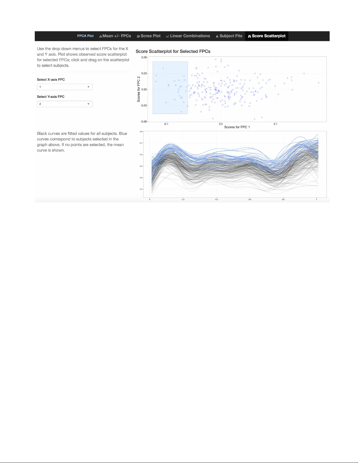
Authors: Julia Wrobel, So Young Park, Ana Maria Staicu
In teractiv e graphics for functional data analyses Julia W rob el 1,* , So Y oung P ark 2 , Ana Maria Staicu 2 , and Jeff Goldsmith 1 1 Departmen t of Biostatistics, Mailman School of Public Health, Columbia Univ ersit y 2 Departmen t of Statistics, North Carolina State Universit y * jw3134@cumc.c olumbia.e du F ebruary 15, 2016 Abstract Although there are established graphics that accompany the most common functional data analy- ses, generating these graphics for each dataset and analysis can be cumbersome and time consuming. Often, the barriers to visualization inhibit useful exploratory data analyses and preven t the develop- men t of in tuition for a metho d and its application to a particular dataset. The refund.shiny pac k age w as dev elop ed to address these issues for sev eral of the most common functional data analyses. After conducting an analysis, the plot shiny() function is used to generate an in teractiv e visualization envi- ronmen t that contains several distinct graphics, man y of which are updated in resp onse to user input. These visualizations reduce the burden of exploratory analyses and can serv e as a useful to ol for the comm unication of results to non-statisticians. Key W ords: F unctional principal comp onen t analysis, m ultilev el functional data, longitudinal functional data, function-on-scalar regression. 1 In tro duction F unctional data analysis (FD A) has b ecome a p opular and useful framew ork for applications in whic h the unit of measurement is a function, curve or image. Conceptually , FDA lev erages the underlying data structure, often temporal or spatial, to impro ve understanding of patterns and v ariation. A wide array of to ols ha ve b een developed for the functional data setting, for example, functional principal comp onent analysis (FPCA) and regression mo dels using functional resp onses ( Ramsay and Silverman , 2005 ; Morris , 2015 ; Sørensen et al. , 2013 ). The basic unit of observ ation is the curv e Y i ( t ) for sub jects i ∈ . . . , I in the 1 cross-sectional setting and Y ij ( t ) for sub ject i at visit j ∈ . . . , J i for the m ultilev el or longitudinal structure. Metho ds for functional data are typically presented in terms of contin uous functions, but in practice data are observed on a discrete grid that may b e sparse or dense at the sub ject level and that may b e the same across sub jects or irregular. Man y metho ds for FDA hav e standard visualization approaches that clarify the results of analyses; examples include scree plots for FPCA and coefficient function plots for function on scalar regression. Clear visualizations aid in exploratory analysis and help to communicate results to non-statistical collab orators. Ho wev er, creating useful plots is often time consuming and must be rep eated eac h time a model is changed, and no soft ware currently exists to facilitate this pro cess. The refund.shiny pack age ( Goldsmith and W robel , 2015 ) creates in teractiv e visualizations for func- tional data analyses, allowing researchers to create common graphics for standard analyses with just a few lines of co de. Curren tly , refund.shiny builds plots for functional principal comp onent analysis (FPCA), m ultilevel FPCA (MFPCA), time-v arying FPCA (TV-FPCA), and function-on-scalar regression (F oSR). The w orkflo w separates analysis and visualization steps: analyses are performed b y functions in the refund pac k age ( Crainicean u et al. , 2015 ) and interactiv e visualizations are generated by the plot shiny() func- tion in the refund.shiny pack age. Changes to the analysis – increasing the num b er of retained principal comp onen ts, for example, or augmen ting a regression mo del with new predictors – are easily incorp o- rated into the graphical interface. User interaction with the displa yed graphics facilitates comparisons and streamlines na vigation b etw een visualizations. W e illustrate the to ols in refund.shiny using a single dataset, whic h we describe briefly here. The diffusion tensor imaging ( DTI ) dataset av ailable in the refund pack age includes cerebral white matter tracts for m ultiple sclerosis patients and health y con trols. White matter tracts are collections of axons, pro jections of neurons that transmit electrical signals and are coated b y a fatt y substance called my elin ( Grev en et al. , 2010 ; Goldsmith et al. , 2011 ; Staicu et al. , 2012 ). DTI is a magnetic resonance imaging mo dalit y that measures diffusion of water in the brain; b ecause w ater mov emen t is restricted in white matter fib ers, DTI allo ws the quantification of white matter tract integrit y . The DTI dataset contains tract profiles – con tin uous summaries of tract prop erties along their ma jor axis – for 142 sub jects across m ultiple visits, with a median of 4 scans p er sub ject. The dataset includes tract profiles for several tracts, 2 the P ASA T score (a contin uous v ariable that indicates brain reactivity and attention span), sub ject sex, sub ject ID, visit num b er, and time of visit ( Strauss et al. , 2006 ). Because w e observe tract profiles for eac h sub ject ov er time, the DTI dataset is a functional dataset with longitudinal structure; in order to use the same dataset across examples we sometimes neglect this structure or subset the data. The following co de can b e used to install refund and refund.shiny and load the DTI data: > install.packages("refund.shiny") > library(refund.shiny) > library(refund) > data(DTI) Sections 2 , 3 , 4 , and 5 each pro vide a brief metho dological ov erview of an analysis technique for FDA and describ e the corresp onding in teractive visualization to ols in the refund.shiny pack age. Section 6 details the structure of the refund.shiny pack age. W e close in section 7 with a discussion. 2 F unctional Principal Comp onen t Analysis W e start with FPCA, one of the most common exploratory to ols for functional datasets. 2.1 FPCA Mo del FPCA c haracterizes modes of v ariabilit y b y decomp osing functional observ ations in to population lev el basis functions and sub ject-sp ecific scores ( Ramsay and Silverman , 2005 ). The basis functions hav e a clear in terpretation, analogous to that of PCA: the first basis function explains the largest direction of v ariation, and eac h subsequent basis function describ es less. The FPCA mo del is typically written Y i ( t ) = µ ( t ) + K X k =1 c ik ψ k ( t ) + i ( t ) (1) where µ ( t ) is the p opulation mean, ψ k ( t ) are a set of orthonormal population-level basis functions, c ik are sub ject-sp ecific scores with mean zero and v ariance λ k , and i ( t ) are residual curves. Estimated basis functions b ψ 1 ( t ) , b ψ 2 ( t ) , . . . , b ψ K ( t ) and corresp onding v ariances b λ 1 ≥ b λ 2 ≥ . . . ≥ b λ K are obtained from a truncated Karh unen-Lo ` ev e decomp osition of the sample cov ariance b Σ( s, t ) = d Co v ( Y i ( s ) , Y i ( t )). In practice, the co v ariance b Σ( s, t ) is often smo othed using a biv ariate smo other that omits entries on the main diagonal 3 to av oid a “n ugget effect” attributable to measurement error, and scores are estimated in a mixed mo del framew ork ( Y ao et al. , 2005 ; Goldsmith et al. , 2013 ). The truncation lag K is often chosen so that the resulting appro ximation accounts for at least 95% of observed v ariance. 2.2 Graphics for FPCA Our example uses the fpca.sc() function from the refund pack age. Sev eral other implementations of FPCA are a v ailable in refund , including fpca.face() , fpca.ssvd() , and fpca2s() , all of which are compatible with refund.shiny . The num b er of functional principal comp onents (FPCs) is chosen by p ercen t v ariance explained, with the default set to 0.99. See ?plot shiny for examples. Graphics for FPCA are implemented by the co de b elow: > fit.fpca = fpca.sc(Y = DTI$cca) > plot_shiny(obj = fit.fpca) Executing this code pro duces a user interface with five tabs. The first tab shows b µ ( t ) ± q b λ k b ψ k ( t ), and includes a drop-do wn men u through whic h the user can select k (an example for a similar tab, based on m ultilevel data, is shown in Section 3 ). The second tab presents static scree plots of the eigenv alues b λ k and the p ercent v ariance explained b y each eigenv alue. The third tab shows b µ ( t ) + P K k =1 c k b ψ k ( t ), and includes slider bars through which the v alues of c k can b e set; adjusting the sliders allows the user to see a fitted curv e for a h yp othetical sub ject with the selected com bination of scores. The fourth tab allo ws users to assess qualit y-of-fit by plotting fitted and observ ed v alues for any sub ject in the dataset. The fifth tab for the in teractive graphic produced b y the co de abov e is shown as a static plot in Figure 1 . A scatterplot of estimated FPC loadings b c ik against b c ik 0 is sho wn in the upper plot, and k and k 0 are selected using drop-do wn menus at the left. The low er plot shows fitted curv es for all sub jects. In the scatterplot, a subset of FPC loadings can b e selected b y clic king-and-dragging to create a blue b ox; blue curv es in the plot of fitted v alues corresp ond to selected sub jects in upp er plot. In Figure 1 the first and second FPCs are selected for the x and y axes of the score plot, respectively , and sev eral sub jects that hav e negativ e v alues for FPC 1 are highligh ted. Fitted v alues for these sub jects are clustered at the top of the y -axis, indicating that the first FPC largely represen ts a vertical shift from the mean. A w orking example of refund.shiny for FPCA on a different dataset is av ailable at h ttps://jeff-goldsmith.shiny apps.io/FPCA . 4 Figure 1: Screenshot showing tab 5 of the in teractive graphics for FPCA. A scatterplot of FPC loadings b c ik against b c ik 0 is shown in the upper plot, and k and k 0 are selected using drop-do wn men us at the left. The lo wer plot sho ws fitted curves for all sub jects. In the scatterplot, a subset of estimated loadings can b e selected by clicking-and-dragging to create a blue b ox; blue curves in the plot of fitted v alues corresp ond to selected p oin ts in upp er plot. 3 Multilev el F unctional Principal Comp onen ts Analysis Multilev el functional principal comp onen t analysis (MFPCA) extends the ideas of FPCA to functional data with a multilev el structure. 3.1 MFPCA Mo del Multilev el functional data are increasingly common in practice; in the case of our DTI example, this structure arises from m ultiple clinical visits made b y eac h sub ject. MFPCA mo dels the within-sub ject correlation induced b y rep eated measures as w ell as the b etw een-sub ject correlation mo deled by classic FPCA. This leads to a t wo-lev el FPC decomp osition, where level 1 concerns sub ject-sp ecific effects and level 2 concerns visit-sp ecific effects. Population-lev el basis functions and sub ject-sp ecific scores are calculated 5 for b oth lev els ( Di et al. , 2009 , 2014 ). The MFPCA mo del is: Y ij ( t ) = µ ( t ) + η j ( t ) + K 1 X k 1 =1 c (1) ik ψ (1) k ( t ) + K 2 X k 2 =1 c (2) ij k ψ (2) k ( t ) + ij ( t ) (2) where µ ( t ) is the p opulation mean, η j ( t ) is the visit-sp ecific shift from the ov erall mean, ψ (1) k ( t ) and ψ (2) k ( t ) are the eigenfunctions for levels 1 and 2, respectively , and c (1) ik and c (2) ij k are the sub ject-specific and sub ject-visit-sp ecific scores. Often, visit-sp ecific means η j ( t ) are not of in terest and can be omitted from the mo del. Estimation for MFPCA extends the approac h for FPCA: estimated b etw een- and within- co v ariances b Σ (1) ( s, t ) = d Co v( Y ij ( s ) , Y ij 0 ( t )) for j 6 = j 0 and b Σ (2) ( s, t ) = d Co v( Y ij ( s ) , Y ij ( t )) are derived from the observed data, smo othed, and decomp osed to obtain eigenfunctions and v alues. Giv en these ob jects, scores are estimated in a mixed-mo del framework. 3.2 Graphics for MFPCA MFPCA is implemen ted in the mfpca.sc() function from the refund pack age. By default, mfpca.sc() do es not calculate visit-means, but they can b e calculated b y sp ecifying the mfpca.sc() argumen t twoway = TRUE . Graphics for MFPCA are implemented by the co de b elow: > Y = DTI$cca > id = DTI$ID > fit.mfpca = mfpca.sc(Y = Y, id = id, twoway = FALSE) > plot_shiny(fit.mfpca) This co de pro duces an interface with fiv e tabs, which is similar to the interface for FPCA but includes features unique to m ultilevel analyses. T abs 1, 2, 3, and 5 for MFPCA are b µ ( t ) ± q b λ ( L ) k L b ψ ( L ) k L ( t ), static scree plots of the estimated eigenv alues b λ ( L ) k L , b µ ( t ) + P K L k L =1 c ( L ) k L b ψ ( L ) k L ( t ), and scatterplots of FPC scores (similar to Figure 1 ), resp ectively . These mirror the tabs for FPCA and include inset sub-tabs to toggle b etw een lev el, L , to displa y results for level 1 or level 2. The fourth tab plots fitted and observ ed v alues for an y user-selected sub ject in the dataset; the user can displa y all visits for the selected sub ject or c ho ose a subset of visits. The first tab for the interactiv e visualization pro duced b y the co de ab ov e is display ed in Figure 2 , and shows b µ ( t ) ± q b λ (1) 2 b ψ (1) 2 ( t ). 6 Figure 2: Screenshot showing tab 1 of the interactiv e graphic for MFPCA. The plot at right shows b µ ( t ) ± q b λ ( L ) k L b ψ ( L ) k L ( t ); k L is chosen by the drop-do wn menu in at left, and the user can switch b etw een level L b y clic king L evel 1 or L evel 2 inset tabs at the top left. 4 Time-v arying F unctional Principal Comp onen t Analysis Time-v arying functional principal component analysis (TV-FPCA) extends the ideas of FPCA to model functional data that are observ ed rep eatedly in a longitudinal framew ork. In contrast to MFPCA, TV- FPCA accounts for the actual time of visit T ij at which the functional ob ject Y ij ( · ) is recorded; this allo ws us to study the time-v arying b ehavior of the underlying true pro cess and mak e predictions of full tra jectory at an unobserved visit time ( Park and Staicu , 2015 ). Other mo deling metho ds for longitudinal functional data that incorp orate the actual visit times T ij include Grev en et al. ( 2010 ) and Chen and M ¨ uller ( 2012 ). 4.1 TV-FPCA Mo del TV-FPCA ( P ark and Staicu , 2015 ) mo del for Y ij ( t ) = Y i ( t, T ij ) is giv en as follows: Y ij ( t ) = µ ( t, T ij ) + K X k =1 c ik ( T ij ) ψ k ( t ) + ij ( t ) , (3) where µ ( t, T ij ) is the p opulation mean that is assumed to v ary smo othly ov er t and visit time T ij , ψ k ( t ) are orthogonal basis functions, c ik ( T ij ) are corresp onding loadings that v ary ov er T ij with mean zero and v ariance λ k , and ij ( t ) are residual curves. The time-v arying scores c ik ( t ij ) are uncorrelated o ver i , but correlated ov er j . Estimation of the TV-FPCA mo del comp onents en tails: 1) estimation of 7 the population mean b y using bi-v ariate smo othing, 2) estimation of the marginal cov ariance Σ( s, t ) = R Co v { Y i ( s, T ) , Y i ( t, T ) } g ( T ) dT , where g ( T ) is the density of the T ij ’s using the observ ed data, smo othing and decomposing it to get the eigenfunctions/eigen v alues b ψ k ( t ) and b λ k ; 3) estimation of the k th comp onen t co v ariance b G k ( T , T 0 ) = Co v { c ik ( T ) c ik ( T 0 ) } . The last step is carried out using either linear random effects, implying c ik ( T ) = b ( k ) 0 i + b ( k ) 1 i T or FPCA implying c ik ( T ) = b ik 1 φ k 1 ( T ) + . . . + b ikL k φ kL k ( T ). By mo deling these longitudinal dynamics, the time-v arying co efficien t function c ik ( · ) can b e used to predict scores at an y longitudinal time T and, as a result, to predict the full resp onse tra jectory Y i ( · , T ). 4.2 Graphics for TV-FPCA TV-FPCA is implemented in the fpca.lfda() function in the refund pack age. In Section 4.1 , we hav e used t to denote the functional argumen t for consistency with the rest of the pap er; ho wev er to main tain consistency with the notations used in P ark and Staicu ( 2015 ), the plot_shiny() function for TV-FPCA uses s to denote the functional argument and T to denote the longitudinal time. Graphics for TV-FPCA are implemented by the co de b elow: > MS <- subset(DTI, case ==1) > index.na <- which(is.na(MS$cca)); Y <- MS$cca; Y[index.na] <- fpca.sc(Y)$Yhat[index.na] > id <- MS$ID > visit.index <- MS$visit > visit.time <- MS$visit.time/max(MS$visit.time) > fit.tfpca <- fpca.lfda(Y = Y, subject.index = id, + visit.index = visit.index, obsT = visit.time, + LongiModel.method = ‘lme’) > plot_shiny(fit.tfpca) The co de pro duces an in terface with tw o tabs. T ab 1 shows exploratory plots and includes three inset sub-tabs. The first sub-tab, sho wn in Figure 3 , plots the observ ed curves for an y user-selected sub ject, and includes options to display the observed curv es of all sub jects in the background and to display the estimated p oint wise mean curv e, denoted by m ( t ). The second sub-tab allo ws the user to see the longitudinal c hanges of the observed curv es for a user-selected sub ject i ; a slider bar animates the sub ject’s visit times and highlights the corresp onding observed curve in the plot. The last sub-tab shows tw o plots of the actual visit times T ij : the b ottom plot presen ts static histogram of visit times of all sub jects, while the top plot presents all of observ ed visit times on a horizon tal line to help visualize the sparsit y of the longitudinal sampling. 8 T ab 2 sho ws estimated mo del components and predictions, and includes 8 inset sub-tabs. Sub-tabs 1 and 2 present static images of the estimated mean surface b µ ( t, T ) and estimated marginal cov ariance b Σ( s, t ). Sub-tabs 3, 4, and 5 illustrate the first step of estimation, and plot estimates of eigenfunctions b ψ k ( t ), m ( t ) ± 2 q b λ k b ψ k ( t ), and static scree plots of the estimated eigen v alues b λ k , respectively . Sub-tab 6 sho ws the estimated co v ariance of the time-v arying loadings c ik ( · ) for user-specified k . Sub-tab 7 sho ws the prediction of c ik ( T ) for any user-selected sub ject i and comp onen t k ; it also has an option of displaying predicted v alues of c ik ( T ) for all sub jects in the background. Lastly , sub-tab 8 shows the prediction of a full resp onse tra jectory Y i ( · , T ) for user-selected sub ject i in animation with change of v alues across 21 equi-spaced grid of p oin ts of T in the range of observ ed visit times of all sub jects. Figure 3: Screenshot sho wing T ab 1 of the in teractive graphic for TV-FPCA. The plot sho ws observ ed data of the selected sub ject. 5 F unction-on-Scalar Regression In many cases, a length p vector of scalar cov ariates x i = [ x i 1 , . . . , x ip ] is observ ed in addition to the function Y i ( t ). In these situations, it is often of interest to mo del the conditional exp ectation of the functional resp onse as it depends on the scalar predictors; indeed, this problem has been the fo cus of a large literature ( Brum back and Rice , 1998 ; Guo , 2002 ; Morris et al. , 2003 ; Morris and Carroll , 2006 ; Reiss et al. , 2010 ; Scheipl et al. , 2015 ; Goldsmith and Kitago , 2015 ; Goldsmith et al. , 2015 ). 9 5.1 F oSR Mo del The most common function-on-scalar regression mo del is Y i ( t ) = β 0 ( t ) + p X k =1 x ik β k ( t ) + i ( t ) (4) where the β k ( t ) are fixed effects asso ciated with scalar cov ariates and the i ( t ) are residual curves. The co efficien ts β k ( t ) are interpreted analogously to co efficients in a (non-functional) m ultiple linear regression – as the exp ected change in resp onse for each one unit change in the predictor – with the exception that they , lik e the outcome, are defined ov er t . Many estimation and inferen tial strategies are a v ailable for mo del ( 4 ); a p opular approac h is to expand co efficien ts β k ( t ) using a spline basis, which allows one to recast ( 4 ) as a traditional linear regression mo del and fo cus estimation on a v ector of unknown spline co efficien ts. Our example uses the bayes fosr() function in the refund pack age, which uses a rich cubic B-spline basis and estimates spline co efficients in a Bay esian framew ork with priors sp ecified to enforce smo othness in the resulting co efficien t functions. Both a Gibbs sampler and a computationally efficien t v ariational approximation are av ailable in refund . 5.2 Graphics for F oSR Graphics for F oSR are implemented by the code b elo w: > DTI = DTI[complete.cases(DTI),] > fit.fosr = bayes_fosr(cca ~ pasat + sex, data = DTI) > plot_shiny(fit.fosr) This co de produces a interface with four tabs, each showing plots associated with mo del 4 . The first tab is a plot of the observed data with the option to color curv es b y a user-selected cov ariate; this builds intuition analogously to scatterplots for non-functional regression. The second tab shows b β 0 ( t ) + P p k =1 x k b β k ( t ), where v alues of x k can b et set b y slider bars for con tinuous cov ariates or drop-do wn men us for categorical co v ariates; adjusting the sliders or drop-do wn men us sho ws the estimated conditional exp ectation for a sp ecified predictor v ector. The third tab, illustrated in Figure 4 , sho ws estimated co efficien t functions b β k ( t ) with p oin twise confidence in terv als for the co v ariate x k selected in a drop-down menu. The fourth tab is a plot of the residual curves b i ( t ) and allows for iden tification of median and outlying curves b y band 10 depth ( Lopez-Pintado and Romo , 2009 ; Sun and Gen ton , 2011 ; Sun et al. , 2012 ); the user can also c ho ose to ’rain b owize by depth’, whic h colors the curves from the median out ward based on depth. Figure 4: Screenshot showing tab 3 of the interactiv e graphic for F oSR. The plot sho ws the estimated co efficien t function b β k ( t ) for the selected cov ariate x k with p oin twise confidence interv als. 6 Co de Structure of the refund.shiny P ac k age W e now briefly describ e the co de infrastructure used to create the refund.shiny pac k age. As indicated in the in tro duction, the w orkflow separates visualization from analysis in the follo wing w ay . First, one analyzes a dataset using a function in the refund pac k age. The functions in refund tak e discretely observed functional data as input, p erform an analysis, and return an ob ject whose class corresp onds to the metho d used. F or example, the fpca.sc() function return as ob ject of class fpca and the bayes.fosr() function returns an ob ject of class fosr . The primary function in refund.shiny , plot shiny() , is a generic function whose b ehavior dep ends on the class of the ob ject passed as an argumen t. Because of this structure, the user exp erience is uniform across a v ariet y of analyses; this also suggests a dev elopment strategy for the addition of interactiv e graphics as new analysis techniques b ecome a v ailable. Lastly , b y separating the analysis and visualization steps, it is p ossible for analysis functions dev elop ed outside of the refund pack age to return ob jects of a defined class and thereby take adv antage of the plotting capabilities we describ e. The interactiv e graphics in the refund.shiny are built on RStudio’s R pack age shiny ( RStudio Inc. , 2015 ), whic h significan tly reduces the barriers to producing webpage-st yle representations of analysis results 11 in R . Other examples of interactiv e graphics that utilize the shiny framework are shinyMethyl ( F ortin et al. , 2014 ) for visualization of high-dimensional genomic data and shinystan ( Stan Dev elopment T eam , 2015 ) for exploring Ba y esian mo dels fit using Mark ov Chain Monte Carlo. In refund.shiny the plots within tabs are pro duced using ggplot2 ( Wickham and Chang , 2015 ); it is p ossible to exp ort each plot as a PDF or to sav e the corresp onding ggplot ob ject to the user’s R w orkspace for further manipulation. 7 Concluding Remarks Visualization has long b een ackno wledged as a central to ol in data analysis. F or functional datasets, the need for useful graphics is compounded: data are inheren tly complex, high-dimensional and structured. Although a robust literature for functional data exists and many metho ds hav e standard graphical represen- tations, the creation of these graphics is often time consuming. The refund.shiny pack age was developed to ease this pro cess by producing a visualization framew ork for several common functional data analyses. By lev eraging new to ols for interactivit y , refund.shiny responds to user input and actions and, in so doing, can build in tuition for analyses in b oth statisticians and practitioners. The in terfaces pro duced b y refund.shiny using the shiny framework are w eb applications, rendered locally b y a web browser. These applications can b e hosted publicly and ma y , in the spirit of “visuanimations“ ( Gen ton et al. , 2015 ), b e included as imp ortan t parts of scientific papers and rep orts. W e use an analytic workflo w that separates mo deling from visualization. Doing so allo ws several meth- o ds and implementations to take adv antage of the same visualization soft ware; as an example, fpca.sc() , fpca.face() , fpca.ssvd() , and fpca2s() implement different metho ds for FPCA but are all compatible with plot shiny() . This pro duces an intuitiv e user exp erience and leav es op en the p ossibility for future approac hes to FPCA or F oSR to use the refund.shiny pac k age for visualization with minimal effort. Sim- ilarly , this workflo w is amenable to the developmen t of in teractive visualizations for additional functional data analyses in future iterations of the pack age. 12 8 Ac kno wledgmen ts The third author’s research w as supp orted partially b y National Science F oundation DMS 0454942 and National Institutes of Health grants R01 NS085211 and R01 MH086633. The last author’s research was sup- p orted in part by Aw ard R01HL123407 from the National He art, Lung, and Blo o d Institute and by Aw ard R21EB018917 from the National Institute of Biomedical Imaging and Bio engineering. The MRI/DTI data w ere collected at Johns Hopkins Universit y and the Kennedy-Krieger Institute. References Brum back, B. and Rice, J. “Smo othing spline mo dels for the analysis of nested and crossed samples of curv es.” Journal of the American Statistical Asso ciation, 93:961–976 (1998). Chen, K. and M ¨ uller, H.-G. “Mo deling Repeated F unctional Observ ations.” Journal of the American Statistical Asso ciation, 107:1599–1609 (2012). Crainicean u, C., Reiss, P ., Goldsmith, J., Gellar, J., J, H., McLean, M. W., Swihart, B., Xiao, L., Chen, Y., Grev en, S., Kundu, M. G., W rob el, J., Huang, L., Huo, L., and Scheipl, F. refund: Regression with F unctional Data (2015). R pack age v ersion 0.1-13. URL http://CRAN.R- project.org/package=refund Di, C.-Z., Crainicean u, C. M., Caffo, B. S., and Punjabi, N. M. “Multilevel F unctional Principal Comp onent Analysis.” Annals of Applied Statistics, 4:458–488 (2009). Di, C.-Z., Crainiceanu, C. M., and Jank, S. J. “Multilev el Sparse F unctional Principal Comp onen t Analy- sis.” Stat, 3:126–143 (2014). F ortin, J. P ., F ertig, E., and Hansen, K. “shin yMethyl: in teractiv e quality con trol of Illumina 450k DNA meth ylation arrays in R [v ersion 1; referees: 2 approv ed].” f1000research, 3:175 (2014). Gen ton, M. G., Castruccio, S., Crippa, P ., Dutta, S., Huser, R., Sun, Y., and V ettori, S. “Visuanimation in statistics.” Stat, 4:81–96 (2015). Goldsmith, J., Bobb, J., Crainiceanu, C. M., Caffo, B., and Reich, D. “P enalized F unctional Regression.” Journal of Computational and Graphical Statistics, 20:830–851 (2011). Goldsmith, J., Greven, S., and Crainicean u, C. M. “Corrected Confidence Bands for F unctional Data using Principal Comp onen ts.” Biometrics, 69:41–51 (2013). Goldsmith, J. and Kitago, T. “Assessing Systematic Effects of Stroke on Motor Control using Hierarchical F unction-on-Scalar Regression.” Journal of the Roy al Statistical So ciety: Series C, T o App ear (2015). Goldsmith, J. and W rob el, J. refund.shiny: Interactiv e plotting for functional data analyses (2015). R pac k age v ersion 0.1. 13 Goldsmith, J., Zipunniko v, V., and Schrac k, J. “Generalized multilev el function-on-scalar regression and principal comp onen t analysis.” Biometrics, 71:344–353 (2015). Grev en, S., Crainiceanu, C. M., Caffo, B., and Reich, D. “Longitudinal F unctional Principal Comp onent Analysis.” Electronic Journal of Statistics, 4:1022–1054 (2010). Guo, W. “F unctional mixed effects mo dels.” Biometrics, 58:121–128 (2002). Lop ez-Pin tado, S. and Romo, J. “On The Concept of Depth for F unctional Data.” Journal of the American Statistical Asso ciation, 104:486–503 (2009). Morris, J. S. “F unctional Regression Analysis.” Annual Review of Statistics and Its Application, 2(1) (2015). Morris, J. S. and Carroll, R. J. “W av elet-based functional mixed mo dels.” Journal of the Roy al Statistical So ciet y: Series B, 68:179–199 (2006). Morris, J. S., V ann ucci, M., Bro wn, P . J., and Carroll, R. J. “W a velet-Based Nonparametric Mo deling of Hierarc hical F unctions in Colon Carcinogenesis.” Journal of the American Statistical Asso ciation, 98:573–583 (2003). P ark, S. and Staicu, A.-M. “Longitudinal functional data analysis.” Stat, 4:212–226 (2015). Ramsa y , J. O. and Silv erman, B. W. F unctional Data Analysis. New Y ork: Springer (2005). Reiss, P . T., Huang, L., and Mennes, M. “F ast F unction-on-Scalar Regression with P enalized Basis Ex- pansions.” International Journal of Biostatistics, 6:Article 28 (2010). RStudio Inc. shiny: W eb Application F ramew ork for R (2015). R pack age v ersion 0.12.2. URL http://CRAN.R- project.org/package=shiny Sc heipl, F., Staicu, A.-M., and Greven, S. “F unctional additive mixed mo dels.” Journal of Computational and Graphical Statistics, T o App ear (2015). Sørensen, H., Goldsmith, J., and Sangalli, L. “An Introduction with Medical Applications to F unctional Data Analysis.” Statistics in Medicine, 32:5222–5240 (2013). Staicu, A.-M., Crainiceanu, C. M., Reich, D. S., and Rupp ert, D. “Modeling functional data with spatially heterogeneous shap e c haracteristics.” Biometrics, 68(2):331–343 (2012). Stan Developmen t T eam. shin ystan: Interactiv e Visual and Numerical Diagnostics and Posterior Analysis for Ba yesian Mo dels (2015). R pack age v ersion 2.0.1. URL http://CRAN.R- project.org/package=shinystan Strauss, E., Sherman, E., and Spreen, O. Comp endium of neuropsyc hological tests: Administration, norms, and commen tary . New Y ork: Oxford Universit y Press (2006). Sun, Y. and Genton, M. G. “F unctional b o xplots.” Journal of Computational and Graphical Statistics, 20(2) (2011). 14 Sun, Y., Gen ton, M. G., and Nychk a, D. W. “Exact fast computation of band depth for large functional datasets: How quickly can one million curv es b e ranked?” Stat, 1(1):68–74 (2012). Wic kham, H. and Chang, W. ggplot2: An Implemen tation of the Grammar of Graphics (2015). R pac k age v ersion 1.0.1. URL http://CRAN.R- project.org/package=ggplot2 Y ao, F., M ¨ uller, H., and W ang, J. “F unctional data analysis for sparse longitudinal data.” Journal of the American Statistical Asso ciation, 100(470):577–590 (2005). 15
Original Paper
Loading high-quality paper...
Comments & Academic Discussion
Loading comments...
Leave a Comment