Multidimensional Scaling in the Poincare Disk

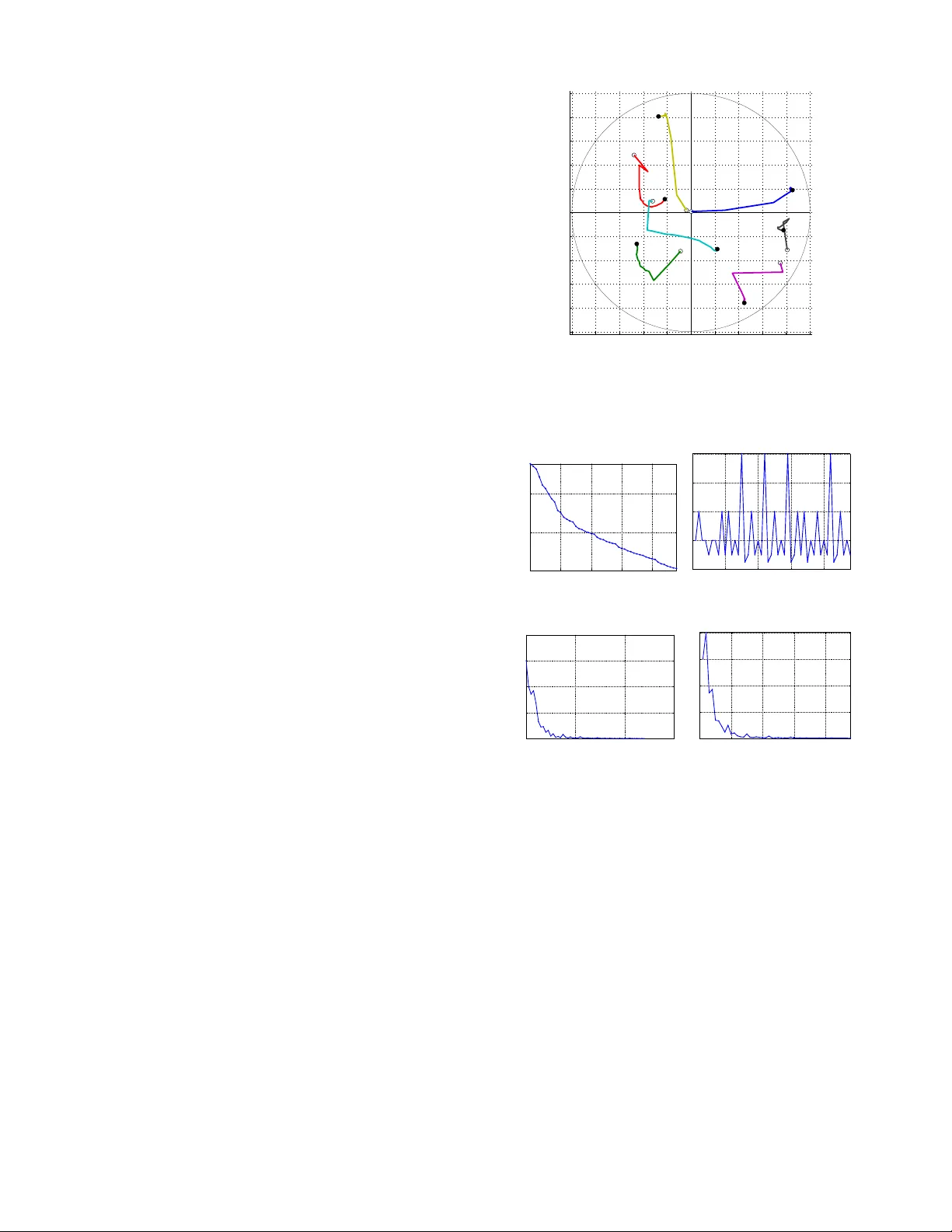
1 Multidimensional Scaling in the Poincaré Disk Andrej CVETK O VSKI, Mark CR O VELLA Abstract —Multidimensional scaling (MDS) is a class of projecti ve algorithms traditionally used in Euclidean space to produce tw o- or three-dimensional visualizations of datasets of multidimensional points or point distances. More recently however , sev eral authors ha ve pointed out that for certain datasets, hyperbolic target space may pro vide a better fit than Euclidean space. In this paper we develop PD-MDS, a metric MDS al- gorithm designed specifically f or the Poincaré disk (PD) model of the hyperbolic plane. Emphasizing the im- portance of proceeding from first principles in spite of the av ailability of various black box optimizers, our construction is based on an elementary hyperbolic line search and rev eals numerous particulars that need to be carefully addressed when implementing this as well as more sophisticated iterativ e optimization methods in a hyperbolic space model. Index T erms —Dimensionality reduction, hyperbolic multidimensional scaling, Poincaré disk, steepest descent, approximate line search, graph embedding I . I N T R O D U C T I O N Metric multidimensional scaling (MDS) [2], [3] is a class of algorithms that take as input some or all of the inter-object distances ( pair dissimilarities ) for n objects and produce as output a point configuration of n points specified by their coordinates in a chosen d -dimensional tar get space . The goal is to return the point configuration whose inter-point distances in the d -dimensional space match as Andrej Cvetkovski was with the Department of Computer Science, Boston Univ ersity , Boston, MA, 02215 USA. E-mail: acvetk@gmail.com. Mark Crovella is with the Department of Computer Sci- ence, Boston Univ ersity , Boston MA, 02215, USA. E-mail: crov- ella@bu.edu. This is an electronic pre-print of an article published in NSP Applied Mathematics & Information Sciences V ol. 10, No. 1, pp. 125-133, 2016, following peer revie w . The definitive publisher- authenticated version is a vailable as [1]. The authors acknowledge the National Science Foundation for supporting this work under Grant no. CNS1018266. closely as possible the original input distances. Usually , this goal is pursued by minimizing a scalar badness- of-fit objective function defined for an arbitrary n -point configuration in the target space; ideally , the output of an MDS algorithm should be the configuration that achie ves the global minimum of the objectiv e function. If the target space dimension is 2 or 3, the output con- figuration can be graphically represented, which makes MDS a visualization tool seeking to preserv e the input distances as faithfully as possible, thus clustering the objects in the target space by similarity . More generally , for a giv en dimension d , metric multidimensional scaling can be used to embed an input set of dissimilarities of the original objects into a d -dimensional metric space. In order to apply MDS, sev eral design decisions must be made. One first needs to choose a tar get metric space of appropriate dimension d and a corresponding distance function. An objective function should be chosen so that it provides a suitable measure of inaccuracy for a gi ven embedding application. If the objectiv e function is nonlinear but satisfies some mild general conditions (smoothness), a numerical optimization method can be chosen for the implementation. A. T arg et space The Euclidean plane is the most common choice of a target space for visualization and other applications due to its simplicity and intuitiveness. Spherical surface can be used, for example, to a void the edge effect of a planar representation [4]. In general, MDS on curved subspaces of Euclidean space can be viewed as MDS in a higher dimensional Euclidean space constrained to a particular surface [5], [6]. A multidimensional scaling algorithm for fitting dis- tances to constant-curv ature Riemannian spaces is gi ven by [7]. This work uses the hyperboloid model of the hy- perbolic space requiring an n + 1-dimensional Euclidean space to represent an n -dimensional hyperbolic space, and is less suitable for visualization purposes. The reader is referred to [8] or [9] for a re view of the history of MDS on Riemannian manifolds of constant or nonconstant curv ature. The use of metric MDS in the hyperbolic plane in the context of interacti ve visualization is proposed by [10], inspired by the focus and conte xt hyperbolic tree vie wer of [11]. The study focuses on the task of embedding higher-dimensional point sets into 2-dimensional config- urations for the purpose of interactiv e visualization. It is demonstrated that the PD has capacity to accommodate lo wer stress embedding than the Euclidean plane. Se veral important pointers to the difficulties one encounters in implementing such algorithms are giv en, b ut a definite specification or implementation is not provided. The adequacy of the hyperbolic spaces for embedding of v arious data is also studied and confirmed in the contexts of network embedding for path cost estimation [12] and routing [13], [14], [15], [16]. B. Objective function A least squares formulation of MDS, to be used in conjunction with an iterativ e numerical method for unconstrained optimization is proposed by [17]. The objecti ve function therein (the Sammon stress criterion) is defined as a normalized sum of the squared dif ferences between the original dissimilarities and the embedded distances of the final point configuration. T o minimize this function, Sammon proposes a descent method with step components calculated using the first two compo- nent deri vati v es of the objectiv e function. [10] adopts Sammon’ s badness-of-fit measure for hy- perbolic MDS b ut observes that applying Sammon’ s iterati ve procedure in the Poincaré disk (PD) using exact deri vati ves is dif ficult due to the complicated symbolic expressions of the second deri v ativ e of the hyperbolic distance function in this model. Subsequently , the Le venber g-Marquardt least squares method is applied in [10], using only first-order deriv ati ves for the opti- mization, but the details of applying this iterati ve method in the Poincaré disk are not elaborated. The proposed method to con vert the seemingly con- strained optimization problem to an unconstrained one by [10] (Eq.12) ensures that the moving configuration would stay inside the model during the optimization. Ho wev er , this transformation fails to follo w the distance 1 2 3 4 1 2 3 4 Figure 1. Comparison of the point trajectories: H-MDS of [10] (left) vs. PD-MDS hyperbolic lines (right) realizing (hyperbolic) lines, or e ven Euclidean lines. The problem is illustrated in Fig. 1. The possibility that the dissimilarity matrix has missing v alues is also not addressed in this work, as the dissimilarities are generated from higher-dimensional points. Input data, ho wev er , may also be sparse. C. PD-MDS In this paper we present PD-MDS, a metric multi- dimensional scaling algorithm using the Poincaré disc (PD) model. For didactic purposes, we complement our exhibition of PD-MDS with a simple steepest decent method with line search. W e show the details of the steepest descent along hyperbolic lines in the PD and present a suitable approximate hyperbolic line search procedure. Based on this dev elopment, we sho w the particulars of a numerical implementation of PD-MDS. PD-MDS is applicable in its own right; additionally , its construction also illustrates some of the specifics that need to be considered when transferring more sophis- ticated iterativ e optimization methods to the PD or to other hyperbolic models. Our numerical experiments indicate that the perfor- mance of a steepest descent method for minimizing a least squares objectiv e on large configurations in the PD is notably dependent on the line search method used, and that binary hyperbolic line search provides markedly better con v ergence and cost properties for PD-MDS compared to more sophisticated or precise methods. The rest of this paper is organized as follo ws. Section II consolidates the notation and concepts from hyperbolic geometry that will be used throughout, and proceeds to de velop two of the building blocks of PD-MDS – steep- est descent in the PD and a corresponding hyperbolic line search. Section III considers particular objectiv e functions and gradients and further discusses properties and applicability of multidimensional scaling in the PD. Section IV pro vides results from the numerical ev alua- tion of the proposed algorithm. Concluding remarks are gi ven in Section V. I I . A D E S C E N T M E T H O D F O R T H E P O I N C A R É D I S K In this section we introduce our notational con ventions and establish some properties of the Poincaré disk that will be used in what follows. W e then proceed to formally define a Poincaré-disk specific descent method and a binary hyperbolic line search, that together make a simple, yet efficient iterati ve minimization method for this model of the hyperbolic plane. A. Preliminaries The P oincaré disk model of the hyperbolic plane is con venient for our considerations since it has circular symmetry and a closed form of the inter-point distance formula exists [18]. W e will be using complex rectangular coordinates to represent the points of the hyperbolic plane, making the PD model a subset of the complex plane C : D = { z ∈ C | | z | < 1 } . (1) The hyperbolic distance between two points z j and z k in D is giv en by d D ( z j , z k ) = 2atanh   z j − z k     1 − z j z k   , (2) where z denotes the complex conjugate. Möbius transformations are a class of transformations of the comple x plane that preserve generalized circles. The special Möbius transformations that take D to D and preserve the hyperbolic distance hav e the form T ( z ) = az + b bz + a , a , b ∈ C , | a | 2 − | b | 2 6 = 0 . (3) Gi ven a point z 0 ∈ D and a direction γ ∈ C with | γ | = 1, we can trav el a hyperbolic distance s ≥ 0 along a hyperbolic line starting from z 0 in the direction γ , arri ving at the point z 0 0 . Lemma 1 . For z 0 ∈ D , γ ∈ C with | γ | = 1, and s ≥ 0, the point z 0 0 = γ tanh s 2 + z 0 z 0 γ tanh s 2 + 1 (i) belongs to the hyperbolic ray passing through z 0 and having direction γ at z 0 , and (ii) d D ( z 0 , z 0 0 ) = s . Pr oof. Given a point z 0 ∈ D and a direction γ ∈ C with | γ | = 1, the hyperbolic ray in D passing through z 0 and having direction γ at z 0 can be parametrized by r ∈ [ 0 , 1 ) as f ( r ) = r γ + z 0 r γ z 0 + 1 . (4) Noting that (4), seen as a function of z = r γ : T ( z ) = z + z 0 zz 0 + 1 is a Möbius transformation taking D to D and preserving hyperbolic distances, we see that d D ( f ( r ) , z 0 ) = d D ( 0 , r ) = ln 1 + r 1 − r whence it follo ws that moving z 0 along a hyper - bolic line in the direction γ by a hyperbolic distance s = ln (( 1 + r ) / ( 1 − r )) we arrive at the point z 0 0 = f  tanh s 2  .  Next, we introduce some of the notation that will be used throughout. • Let the point configuration at iteration t = 1 , 2 , . . . T consist of n points in the Poincaré disk D z j ( t ) , j = 1 . . . n represented by their rectangular coordinates: z j ( t ) = y j , 1 ( t ) + iy j , 2 ( t ) , i = √ − 1 , y j , 1 , y j , 2 ∈ R with   z j ( t )   < 1 . • W e also use vector notation to refer to the point configuration z ( t ) =  z 1 ( t ) z 2 ( t ) . . . z n ( t )  T = y 1 + i y 2 = =  y 1 , 1 ( t ) y 2 , 1 ( t ) . . . y n , 1 ( t )  T + i  y 1 , 2 ( t ) y 2 , 2 ( t ) . . . y n , 2 ( t )  T , where [ · ] T in this work indicates the real matrix transpose (to be distinguished from the complex conjugate transpose.) • The distance matrix for a gi ven point configuration z is the real valued symmetric matrix D ( z ) =  d jk  n × n whose entry d jk is the hyperbolic distance between points z j and z k in the configuration z : d jk = d D ( z j , z k ) . • The dissimilarity matrix ∆ =  δ jk  n × n is a symmet- ric, real-valued matrix containing the desired inter- point distances of the final output configuration (the dissimilarities ). The diagonal elements are δ j j = 0 and all other entries are positi ve real numbers: δ jk = δ k j > 0 for j 6 = k . • The indicator matrix I =  I jk  n × n is a symmetric 0-1 matrix, used to allo w for missing dissimilarity v alues. The entries of I corresponding to missing v alues in ∆ are set to 0. All other entries are set to 1. • The weight matrix W =  w jk  n × n is a symmetric, real-v alued matrix introduced to enable weighting of the error terms for individual pairs of points in the objecti ve function sum. For con venience, w jk corresponding to missing dissimilarities are set to some finite v alue, e.g. 1. • The objective function to be minimized is the embedding err or function E t = E t ( z , ∆ , W , I ) that, gi ven the sets of dissimilarities and weights, as- sociates to a configuration z an embedding error E t . An example of an error function is the sum of relati ve squared differences E t ( z , ∆ , W , I ) = n ∑ j = 1 n ∑ k = j + 1 w jk I jk  d jk ( t ) − δ jk δ jk  2 . (5) The objectiv e function can optionally be normalized per pair by dividing with the number of summands  n 2 − n  / 2. B. Descent in the P oincaré disk Gi ven a configuration of points z , matrices ∆ , W , and I , the distance function d D ( z j , z k ) , and an objectiv e function E ( z , ∆ , W , I ) , define g = ∇ E def =        ∂ E ∂ y 1 , 1 + i ∂ E ∂ y 1 , 2 ∂ E ∂ y 2 , 1 + i ∂ E ∂ y 2 , 2 . . . ∂ E ∂ y n , 1 + i ∂ E ∂ y n , 2        =      g 1 g 2 . . . g n      . (6) According to Lemma 1, moving the points z 1 , . . . , z n of the configuration z along distance realizing paths in the PD defined respecti vely by the directions − g 1 , . . . , − g n at z (Fig. 2) will result in configuration z 0 with points z 0 j = − rg j + z j − rg j z j + 1 (7) where r ≥ 0 is the step-size par ameter which determines the hyperbolic distances s j trav eled by z j : s j = ln 1 + r   g j   1 − r   g j   . (8) 1 2 3 4 Figure 2. An example of moving a 4-point configuration in a given (descent) direction along distance realizing paths of the Poincaré disk The PD model (1) implies the constraints   z j   < 1 for the point coordinates. Still, the optimization on the PD can be vie wed as unconstrained by observing that the constraints    z 0 j    < 1 will not be violated while moving a configuration z in D if the distances s j trav eled by each point are always kept finite, i.e. s M = max j s j < ∞ . (9) Since (9), according to (8), corresponds to r max j   g j   < 1, we hav e the constraint on r r < 1 k g k ∞ . When implementing iterative descent minimization methods with line search in the Poincaré disk, it is important to specify a hyperbolic distance window s M along the descent lines where the next configuration will be sought. In this case the corresponding v alue of the parameter r is r M = 1 k g k ∞ · tanh s M 2 < 1 k g k ∞ . (10) Since the Poincaré disk model is conformal, following the direction − g (the opposite of (6)) corresponds to the steepest descent optimization method. Moving the point configuration along hyperbolic lines (distance realizing paths), on the other hand, ensures that the steepest descent direction is exhausted most ef ficiently giv en the current information about the objectiv e function. C. A steepest descent algorithm for the PD Figure 3 sho ws a framew ork for PD-MDS. The input data of PD-MDS consists of the initial con- figuration z ( 1 ) , and the input metric: the dissimilarities Algorithm PD-MDS Input data: an initial configuration z ( 1 ) the dissimilarities ∆ , weights W , indicators I Input parameters: an objecti ve function E ( z , ∆ , W , I ) the stopping tolerances ε E , ε ∆ E , ε g , ε r , T M Output: a final point configuration z ( T ) a final embedding error E T Initialize: t ← 1; s M ← 10; E − 1 ← ∞ ; z ← z ( 1 ) ; . . . . . . . {3.1} Loop: E ← E ( z , ∆ , W , I ) ; g ← ∇ E ( z , ∆ , W , I ) ; . . . . . {3.2} r M ← 1 k g k ∞ · tanh s M 2 ; . . . . . . . . . . . . . . . . . . . . . . . . {3.3} Break if E < ε E or E − 1 − E < ε ∆ E or k g k ∞ < ε g or r M < ε r or t > T M ;            . . . . . . . . . . . . . . {3.4} E − 1 ← E ; r ← HypLineSearch ( E ( z , ∆ , W , I ) , − g , 0 , r M ) ; . {3.5} ∀ j ∈ { 1 .. n } , z j ← − rg j + z j − rg j z j + 1 ; . . . . . . . . . . . . . . . . . {3.6} t ← t + 1; Return z ( T ) ← z and E T ← E ( z , ∆ , W , I ) . Figure 3. PD-MDS ∆ with the associated weights W and the indicators of missing dissimilarities I . The input parameters are the objectiv e error function E ( z , ∆ , W , I ) and the stopping tolerances ε E , ε ∆ E , ε g , ε r , and T M . The output of PD-MDS consists of the final point configuration z ( T ) and its associated embedding error E T = E ( z ( T ) , ∆ , W , I ) . The initialization {3.1} sets the maximum hyperbolic distance s M that can be trav eled by any point of the configuration, and the previous v alue of the embedding error E − 1 . Each iteration starts by determining the gradient of the error in the current configuration {3.2} and the corresponding windo w r M {3.3} for the parameter r (Eq. (10)). A hyperbolic line search (described in Sec. II-D) is performed {3.5} in the direction of the steepest descent − g of the embedding error and the resulting step- size parameter r is used in {3.6} to arri ve at the next configuration as in (7). Se veral stopping criteria are used (line {3.4}) to terminate the search. Ideally , the algorithm exits when the embedding error is close to 0 ( E < ε E ). T ermination also occurs in the cases when the error decreases too slo wly ( E − 1 − E < ε ∆ E ), or when the gradient or the step- ping parameter become too small ( k g k ∞ < ε g , r M < ε r ). Finally , T M , the maximum allowed number of iterations, is used as a guard against infinite looping. The line sear ch subprogram used in {3.5} is described next. D. Appr oximate hyperbolic line sear ch An exact line sear ch could be used in line {3.5} (Fig. 3) to determine a v alue for the step size r such that the corresponding new configuration {3.6} achieves a local minimum of the embedding error along the search path with tight tolerance: r ≈ argmin r ∈ [ 0 , r M ] q ( r ) , (11) where q ( r ) is the embedding error as a function of r . Ho wev er , increasing the precision of this computation is not essential to the conv ergence performance since the steepest descent search direction is only locally optimal. Further , exact line search can fail to con ver ge to a local minimum e ven for a second degree polynomial due to finite machine precision [19]. On the other hand, appr oximate line sear ch generally provides con vergence rates comparable to the exact line search while significantly reducing the computational cost per line search. In fact, the step calculation used in [17] is a “zero-iteration” approximate line search, where the step size is simply guessed based on the first two deri vati v es of the error . Concei vably , the simplest inexact step calculation would guess the step size based only on the directional gradient at the current configuration. Approximate line search procedures aim to reduce the computational cost of determining the step parameter by posing weaker conditions on the found solution: Rather than searching for a local or global minimizer of q ( r ) on ( 0 , r M ] , a value is returned by the line search function as satisfactory if it provides sufficient decrease of the objecti ve function and suf ficient progress to ward the solution configuration. A common approach to defining suf ficient decrease is to define the “roof ” function λ ( r ) = q ( 0 ) + p · q 0 ( 0 ) · r , 0 < p < 1 (12) r pq ′ ( 0 ) slope q ′ ( 0 ) slope acceptable acceptable λ ( r ) q(r) r M Figure 4. Acceptable step lengths for inexact line search obtained from the sufficient decrease condition. which is a line passing through ( 0 , q ( 0 )) and ha ving a slope which is a fraction of the slope of q ( r ) at r = 0. W ith this function, we define that sufficient decrease is provided by all values of r such that q ( r ) < λ ( r ) , r ∈ ( 0 , r M ] (13) Fig. 4 shows an example of acceptable step length segments obtained from the sufficient decrease condition (13). T o ensure suf ficient progress, we adopt a binary search algorithm motiv ated by the simple backtracking approach (e.g. [20]). The details are giv en in Fig. 5. Procedur e HypLineSearch Input data: an initial guess of the step parameter r 0 the maximum step value r M the function q ( r ) Input parameters: the slope parameter p for the roof function λ ( r ) ; Output: an acceptable step parameter r Initialize: r ← r 0 ; While r < r M and q ( r ) < λ ( r ) , r ← 2 · r ; . . . . . . . . . . . . . . . . . . . . . . . . . . . . . . . . . . {5.1} While r < r M or q ( r ) > λ ( r ) , r ← r / 2; . . . . . . . . . . . . . . . . . . . . . . . . . . . . . . . . . . . {5.2} Return r . Figure 5. Line search procedure for PD-MDS W e start the line search with an initial guess r 0 for the step size parameter , and in the expansion phase {5.1} we double it until it violates the window r M or the suf ficient decrease condition. In the reduction phase {5.2}, we halve r until it finally satisfies both the windo w requirement r < r M and the decrease criterion q ( r ) < λ ( r ) . W e observ e that, when started at a point with nonzero gradient, the line search will always return a nonzero v alue for r . Since the returned acceptable step r is such that the step 2 · r is not acceptable, there will be a maximum acceptable point r m from the same acceptable segment as r , such that r ≤ r m < 2 · r , whence r > r m / 2. In other words, the returned v alue is always in the upper half of the interval [ 0 , r m ] and we accept this as sufficient progress to ward the solution, thus eliminating some more computationally demanding progress criteria that would require calculation of q 0 ( r ) at points other than r = 0 or cannot always return a nonzero r [20], [19]. It remains to show how to calculate the slope of λ ( r ) , that is pq 0 ( 0 ) (Eq. 12). Giv en a configuration z and a direction − g = − ∇ E ( z , ∆ , W , I ) , the configuration z 0 as a function of r (7) can be conv eniently represented as a column-vector function M ( − r g , z ) (14) whose j -th entry is the Möbius transform M j ( r ) = − rg j + z j − rg j z j + 1 . The associated embedding error as a function of r is then q ( r ) = E ( M ( − r g , z ) , ∆ , W , I ) , (15) and it can be easily shown that its slope is giv en by q 0 ( r ) = d d r q ( r ) = =  Re M 0 ( − r g , z )  T Re ∇ E ( M ( − r g , z ) , ∆ , W , I ) +  I m M 0 ( − r g , z )  T I m ∇ E ( M ( − r g , z ) , ∆ , W , I ) where the entries of M 0 ( − r g , z ) are given by M 0 j ( r ) = d d r M j ( r ) = g j   z j   2 − 1 ( 1 − rg j z j ) 2 . W e thus ha ve a general explicit formula for calculating q 0 ( r ) gi ven a configuration z and the corresponding gradient g of E at z . In particular , this formula can be used to calculate pq 0 ( 0 ) , the slope of λ ( r ) . I I I . M U LT I D I M E N S I O N A L S C A L I N G I N T H E P D A. Objective functions and gradients The iterati ve minimization method presented in Sec. II requires a choice of an embedding error function with continuous first deriv atives. In this work we consider the least squares error function E = c n ∑ j = 1 n ∑ k = j + 1 c jk  d jk − a δ jk  2 . (16) W e note that (16) is a general form from which se veral special embedding error functions can be obtained by substituting appropriate v alues of the constants c , c jk , and a . Examples include: • Absolute Differences Squared (ADS) E = n ∑ j = 1 n ∑ k = j + 1 w jk  I jk  d jk − a δ jk  2 (17) • Relati ve Differences Squared (RDS) E = n ∑ j = 1 n ∑ k = j + 1 w jk  I jk d jk − a δ jk a δ jk  2 (18) • Sammon Stress Criterion (SAM) E = 1 a n ∑ j = 1 n ∑ k = j + 1 I jk δ jk · n ∑ j = 1 n ∑ k = j + 1 w jk  I jk  d jk − a δ jk  2 a δ jk (19) As the most general case of (16), individual importance dependent on the input dissimilarities can be assigned to the pairwise error terms using the weights terms w jk . PD-MDS also requires calculation of the gradient of the error function. For a general error function, closed form symbolic deriv atives may or may not exist. In any case, one can resort to approximating the gradient using finite difference calculations. Numerical approximation may also hav e lower computational and implementation costs than the formal deri v ativ es. Ho we ver , the use of nu- merical deriv atives can introduce additional conv ergence problems due to limited machine precision. For the sum (16), a symbolic deriv ation of the gradient of (16), including both the Euclidean and hyperbolic cases, can be easily carried out and is omitted here for bre vity . From the obtained result, symbolic deriv ati ves of (17)–(19), as well as any other special cases deriv able from (16) can be obtained by substituting appropriate constants. B. Local vs. global minima PD-MDS, being a steepest descent method that termi- nates at near-zero progress, can find a stationary point of the objectiv e function. In the least squares case, if the v alue at the returned solution is close to zero (that is, E < ε E ), then the final configuration can be considered a global minimizer that embeds the input metric with no error . In all other cases, a single run of PD-MDS cannot distinguish between local and global points of minimum or between a minimizer and a stationary point. A common way of getting closer to the global minimum in MDS is to run the minimization multiple times with dif ferent starting configurations. Expectedly , there will be accumulation of the results at several v alues, and the more values are accumulated at the lowest accumulation point, the better the confidence that the minimal value represents a global minimum i.e. the least achiev able embedding error . Numerous methods that are more likely to find a lower minimum than the simplest repeated descent methods in a single run ha ve been contemplated in the numerical optimization literature. Ho we ver , to guarantee in general that the global minimizer is found is difficult with any such method. It may be necessary to resort to running the sophisticated methods sev eral times as well in order to gain confidence in the final result. Since these methods are usually computationally more comple x or incorporate a larger number of heuristic parameters, the incurred computational and implementational costs often of fset the benefits of their sophistication. C. Dissimilarity scaling The objective functions used in metric Euclidean MDS are typically constructed to be scale-in variant in the sense that scaling the input dissimilarities and the coordinates of the output configuration with the same constant factor a does not change the embedding error . This is possible for Euclidean space since the Euclidean distance function scales by the same constant factor as the point coordinates: L ∑ s = 1 ( a · y js − a · y ks ) 2 ! 1 / 2 = a · d jk . Thus, for example, if d jk is the Euclidean distance, then the sums (18) and (19) are scale-inv ariant, whereas (17) is not. Ho wev er , when d jk is the hyperbolic distance function (2), none of the (17)–(19) are scale-in variant. Therefore, the simplest ADS error function (17) may be a prefer- able choice for reducing the computational cost in the hyperbolic case. The lack of scale-inv ariance of the hyperbolic distance formula (2) implies an additional de gree of freedom in the optimization of the embedding error – the dissimi- larity scaling factor . In Eqs. (16)–(19) this extra degree of freedom is captured via the parameter a that scales the original entries of the dissimilarity matrix. I V . N U M E R I C A L R E S U LT S A. A synthetic example T o illustrate the functioning of PD-MDS, we provide an example random configuration consisting of sev en points in the Poincaré disk. T o carry out this experiment, we populate the in- put dissimilarity matrix with the hyperbolic inter-point distances and start PD-MDS from another randomly- generated se ven point initial configuration in the PD. Fig. 6 shows the trajectories trav eled by the points during the minimization. The clear points denote the initial configuration, whereas the solid ones represent the final point configuration. The operation of the PD-MDS algorithm as it iterates ov er the provided example configuration is examined in detail in Fig. 7. The figure shows the PD-MDS internal parameters vs. the iteration number: In Fig. 7a, the embedding error E monotonically decreases with ev ery iteration; the iterations terminate at the fulfillment of E < ε E = 10 − 6 , which means that likely the output configuration represents the global minimum and the final inter-point distances match the input dissimilarities very closely . The step-size parameter r is initialized with a value of 1 and assumes only v alues of the form 2 k , for integral k (Fig. 7b). The exponential character of the change of r in accord with {5.1} and {5.2} (Fig. 5) ensures the low computational cost of the line search subprogram. The refining of the step size as the current configura- tion approaches a local minimum of the error function, on the other hand, is achie ved by the decrease of the gradient norm. This is further illustrated in Figs. 7c and 7d. In our pool of numerical experiments, we produced graphs similar to those shown in Fig. 7 while using two −1 −0.8 −0.6 −0.4 −0.2 0 0.2 0.4 0.6 0.8 1 −1 −0.8 −0.6 −0.4 −0.2 0 0.2 0.4 0.6 0.8 1 1 2 3 4 5 6 7 1 2 3 4 5 6 7 Figure 6. The minimization trajectory for a sev en point configuration using PD-MDS. The clear and the solid points are respectively the initial and the final point configuration. 0 10 20 30 40 10 −6 10 −4 10 −2 (a) Embedding error E Iterations 0 10 20 30 40 0 2 4 6 8 (b) Step−size parameter r Iterations 0 20 40 60 0 0.1 0.2 0.3 0.4 (c) Norm of gradient ||g|| ∞ Iterations 0 10 20 30 40 0 0.2 0.4 0.6 0.8 (d) Rel. step−size parameter r/r M Iterations Figure 7. The PD-MDS internal parameters vs. the iteration number for the seven point example of Fig. 6: (a) the embedding error E , (b) the step-size parameter r , (c) the norm of the gradient k g k ∞ , and (d) the step-size parameter relative to the maximum allowed value r / r M . other line search strategies: (i) exact search and (ii) line search using an adaptiv e approximate step-size parame- ter . Both of these strategies sho wed slower con v ergence compared to the binary hyperbolic line search, and were of higher computational cost. B. Scaling of the Iris dataset in the PD As a first experiment on real-w orld data, we apply PD- MDS to the Iris dataset [21]. This classical dataset con- sists of 150 4-dimensional points from which we extract the Euclidean inter-point distances and use them as input dissimilarities. The embedding error as a function of the 10 −2 10 −1 10 0 10 1 0.3 0.35 0.4 0.45 0.5 0.55 0.6 Hyperbolic Scaling of the Iris Dataset Embedding error Input scaling factor a Figure 8. The ef fect of scaling of the dissimilarities on the embedding error for the Iris Dataset [21]. The input dissimilarities are the Euclidean distances between pairs of original points. This PD-MDS result rev eals that the Iris dataset is better suited for embedding to the hyperbolic plane that to the Euclidean plane. scaling factor a is sho wn in Fig. 8. Each value in the diagram is obtained as a minimum embedding error in a series of 100 replicates starting from randomly chosen initial configurations. Minimal embedding error o verall is achie ved for a ≈ 4. The improvement with respect to the 2-dimensional Euclidean case is 10%. Thus, the Iris dataset is an ex- ample of dimensionality reduction of an original higher - dimensional dataset that can be done more successfully using the PD model. V . C O N C L U S I O N In this paper , we elaborated the details of PD-MDS, an iterati ve minimization method for metric multidimen- sional scaling of dissimilarity data in the Poincaré disk model of the hyperbolic plane. While our exposition concentrated on a simple steepest descent minimization with approximate binary hyperbolic line search, we belie ve that elements of the presented material will also be useful as a general recipe for transferring other , more sophisticated iterativ e methods of unconstrained optimization to v arious models of the hyperbolic space. A C K N O W L E D G E M E N T The authors acknowledge the National Science Foun- dation for supporting this work under Grant no. CNS- 1018266. R E F E R E N C E S [1] Andrej Cvetkovski and Mark Crovella. Multidimensional scal- ing in the Poincaré disk. Applied Mathematics & Information Sciences , 10(1):125, 2016. [2] T . F . Cox and M. A. A. Cox. Multidimensional Scaling (Monographs on Statistics and Applied Probability) . Chapman & Hall/CRC, 2nd edition, 2000. [3] I. Borg and P . J. F . Groenen. Modern Multidimensional Scaling: Theory and Applications (Springer Series in Statistics) . Springer , Berlin, 2nd edition, 2005. [4] T . F . Cox and M. A. A. Cox. Multidimensional scaling on a sphere. Communications in Statistics , 20:2943–2953, 1991. [5] P . M. Bentler and D. G. W eeks. Restricted multidimensional scaling models. J . Math. Psychol. , 17:138–151, 1978. [6] B. Bloxom. Constrained multidimensional scaling in N-spaces. Psychometrika , 43:397–408, 1978. [7] H. Lindman and T . Caelli. Constant curvature Riemannian scaling. J . Math. Psychol. , 2:89–109, 1978. [8] J. D. Carroll and P . Arabie. Multidimensional scaling. Ann. Rev . Psychol. , 31:607–649, 1980. [9] J. De Leeuw and W . Heiser . Theory of multidimensional scaling. In P . R. Krishnaiah and L. N. Kanal, editors, Handbook of statistics , volume 2. North-Holland, 1982. [10] J. A. W alter . H-MDS: a new approach for interactiv e visual- ization with multidimensional scaling in the hyperbolic space. Information Systems , 29(4):273 – 292, 2004. [11] J. Lamping and R. Rao. Laying out and visualizing large trees using a hyperbolic space. In UIST ’94: Proceedings of the 7th annual A CM symposium on User interface software and technology , pages 13–14, New Y ork, NY , USA, 1994. ACM. [12] Y . Shavitt and T . T ankel. Hyperbolic embedding of Inter- net graph for distance estimation and overlay construction. IEEE/A CM T rans. Netw . , 16(1):25–36, Feb. 2008. [13] R. Kleinberg. Geographic routing using hyperbolic space. In Pr oceedings of IEEE Infocom 2007 , pages 1902–1909, May 2007. [14] D. Krioukov , F . Papadopoulos, M. Boguñá, and A. V ahdat. Greedy forwarding in scale-free networks embedded in hyper - bolic metric spaces. SIGMETRICS P erform. Eval. Rev . , 37:15– 17, October 2009. [15] A. Cvetkovski and M. Crovella. Hyperbolic embedding and routing for dynamic graphs. In Pr oceedings of IEEE Infocom 2009 , pages 1647–1655, Apr 2009. [16] F . Papadopoulos, D. Krioukov , M. Boguñá, and A. V ahdat. Greedy forwarding in dynamic scale-free networks embedded in hyperbolic metric spaces. In INFOCOM, 2010 Proceedings IEEE , March 2010. [17] J. W . Sammon. A nonlinear mapping for data structure analysis. IEEE T rans. Comput. , C-18(5):401–409, May 1969. [18] J. W . Anderson. Hyperbolic Geometry . Springer , 2nd edition, 2007. [19] P . E. Frandsen, K. Jonasson, H. B. Nielsen, and O. Tinglef f. Unconstrained Optimization . IMM, DTU, 3rd edition, 2004. [20] J. Nocedal and S. J. Wright. Numerical Optimization . Springer , 1999. [21] E. Anderson. The irises of the Gaspé peninsula. Bulletin of the American Iris Society , 59:2–5, 1935.