The Degree Distribution of Random Birth-and-Death Network with Network Size Decline
In this paper, we provide a general method to obtain the exact solutions of the degree distributions for RBDN with network size decline. First by stochastic process rules, the steady state transformation equations and steady state degree distribution…
Authors: Xiaojun Zhang, Huilan Yang
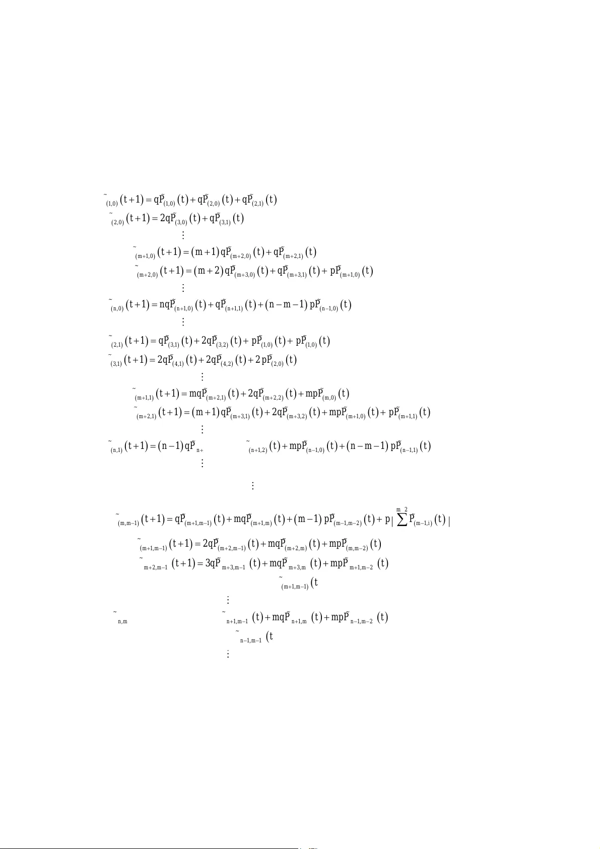
Th e D egr ee Distr ibu tion of Ra n d om B i r th -a n d-D ea th Netw or k w ith N etw or k S iz e D ec li n e Xi aojun Zhang * , Hui l an Y ang School of Mathemati cal Sci ences, Uni versi ty of El ectroni c Sci ence and Technol og y of Chi na, Cheng du 61 1731 , P . R. Chi na A b s tr act In thi s paper , we provi de a g eneral method to obtai n the ex act sol uti on s of the deg ree di stri buti ons for RBDN wi th network si ze decl i ne . Fi rst by stochasti c process rul es , the steady state transformati on equati ons and steady state deg ree di stri buti on equati ons are g i ven i n t h e c a s e of m ≥ 3 , 0< p <1/2 , then the averag e deg ree of network wi th n nodes i s i ntroduced to cal cul ate the deg ree di stri buti on . Especi al l y , taki ng m =3 as an ex ampl e, we expl ai n the detai l ed sol vi ng process, i n whi ch computer si mul ati on i s used to veri fy our deg ree di stri buti on sol uti ons. In addi ti on, the tai l characteri sti cs of the deg ree di stri buti on are di scussed. Our fi ndi ng s sug g est t h a t the deg ree di stri buti ons wi l l exhi bi t P oi sson tai l property for the decl i ni ng RBDN. K e y wor d s: random bi rth- and -death network (RBDN), stochas ti c p rocesses, Markov chai n, g enerati ng functi on, deg ree di stri buti on * Correspondi ng author: Xi aojun Zhang Emai l address: sczhx j@uestc.edu. cn Th e D egr ee D istr i bu tion of Ra ndom B ir th-a n d -D ea th Netw or k w ith Netw or k Siz e D ec li n e 1. In tro du c ti on In the real worl d, there ex i st many bi rth- and -death networks such as the W orl d W i de W eb [1 - 3], the communi cati on networks [4-6], the fri end rel ati onshi p networks [7-10] and the food chai n networks [1 1-13] , i n whi ch nodes may enter or ex i t at any ti me . For thi s ki nd of evol vi ng networks , the deg ree di stri buti on i s al ways one of the most i mportant stati sti cal properti es. Several methods h ave been proposed to cal cul ate the ir deg ree di stri buti ons l i ke the fi rst-order parti al -di fferenti al equati on method by Sal dana [14], the mean -fi el d approach [15] by Sl ater et al . [ 1 6 ] , the r a t e e q u a t i o n approach by Sarshar and Roychowdhury [ 17] Moore et al . [18], Garci a-Domi ng o et al . [19] Ben- Nai m and Krapi vsky [ 20]. Whi l e these approaches ai m at the networks whose si ze i s g rowi ng or remai n unchang ed at each ti me step keep , Zhang et al . [21] put forward the stochasti c proces s r u l e s (S P R) based Markov chai n method to sol ve evol vi ng network s i n whi ch the network si ze may i ncrease or decrease at each ti me step. Furthermore, a random bi rth- and -death network model (RBDN) i s consi dered [22 ], i n whi ch at each ti me step, a new node i s added i nto the network wi th probabi l i ty p (0< p <1) wi t h connect i o n to m ol d nodes uni form ly , or an ex i sti ng node i s del eted from the network wi th the probabi l i ty q =1 - p . For network si ze decl i ne (0< p <1/2), si nce m i s a cri ti cal parameter for the deg ree di stri buti ons, sol uti on methods may vary for di fferent m . Whi l e Zhang et al . [22 ] onl y consi der a speci a l c a s e m = 1 , 2 , i n thi s paper , a g eneral approach i s proposed for sol vi ng the deg ree di stri buti ons of R BDN wi th network si ze decl i ne i n case of m ≥ 3 . Taki ng m =3 as an ex ampl e, we provi de the ex act sol uti on s o f the deg ree di stri buti ons . Our fi ndi ng s al so i ndi cate that the tai l of the deg ree di stri buti on for the decl i ni ng RBDN i s subject to P oi sson tai l . Th is paper i s structured as fol l ows: Secti on 2 g i ves the RBDN model wi th 0 < p <1/2 and i ts steady -state equati ons ; Secti on 3 provi des the method of sol vi ng deg ree di stri buti on of RBDN w i t h 0< p <1/2; Secti on 4 further di scusses the tai l characteri sti cs of the deg ree di stri buti on and Secti on 5 concl udes the paper . 2. St e ady S t a te Equa t i ons o f R B D N w i th N e t w o rk Si z e De c l i ne 2.1 RB DN m od e l Consi der the RBDN model [ 22]: (i ) T he i ni ti al network i s a compl ete g raph wi th m +1 nodes, where m i s a posi ti ve i nteg er ; (ii ) A t each uni t of ti me, add a new node to the network wi th probabi l i ty p (0 < p <1/2) and connect i t wi th m ol d nodes uni form ly , or randoml y del ete a node from the network wi th probabi l i ty q =1 - p . Note: (a) Here we assume the l ow-bound of the network si ze 0 1 n , that i s , i f the number of nodes i n the network i s 0 n at ti me t , then at ti me 1 t , we onl y add a new node to the network w i t h probabi l i ty p and connect i t to the ol d node i n the network. (b) If at ti me t , a new node i s added to the network and the network si ze i s l ess than m , then t h e new node i s connected to al l ol d nodes. 2.2 Ste ad y s t ate t r an s f or m ati on e q u at i on s Usi ng SP R [21] , we use , nk to descri be the state of node v , where n i s t h e n u m b e r o f nodes i n the network that contai ns v , and k i s the deg ree of node v . Let NK t denote the state of node v at ti me t , the stochasti c process ,0 N K t t i s an erg odi c aperi odi c homog eneous Markov chai n wi th the state space , , 1 , 0 1 E n k n k n . Let t P be the probabi l i ty di stri buti on of NK t , i . e. , , nk P t P NK t n k (1) T he s tate transformati on equati ons are as fol l ows (see the A ppendi x for the detai l s ): +1 tt P P P (2) where P i s the one-step transi ti on probabi l i ty matri x . L et , lim , ik t P N K t i k (3) Taki ng the l i mi t of Eq. (2) as + t , the steady state transformati on equati ons can be obtai ned 1,0 1,0 2 ,0 2,1 2 ,0 3,0 3, 1 1,0 2 ,0 2 , 1 2 ,0 3,0 3, 1 1,0 ,0 1,0 1, 1 1,0 22 11 22 1 m m m m m m m n n n n q q q qq m m q q m m q q p n nq q n m p (4) 2 , 1 3,1 3, 2 1,0 1,0 3, 1 4 , 1 4 ,2 2 ,0 1, 1 2,1 2 , 2 ,0 2 , 1 3, 1 3,2 1,0 1 ,1 , 1 1, 1 1 , 2 1,0 1, 1 22 3 2 2 2 12 2 1 2 1 2 1 m m m m m m m m m n n n n n q q p p q q p m mq q mp m m q q mp p nP n q q mp n m p ( 5) 2 , 1 1, 1 1, 1, 2 1, 0 1, 1 2 , 1 2, , 2 2 , 1 3, 1 3, 1, 2 1, 1 , 1 1, 1 1, 1, 1 12 2 3 + 2 1 1 m m m m m m m m m m i i m m m m m m m m m m m m m m m m m m n m n m n m n m m q mq m p p m q mq m p m q mq mp m m p n n m q mq m p 2 1, 1 1 nm n m p 1 1, 2, 2 , 1 , 1 , 0 2 , 3, 3, 1 1, 1 1, 1, 0 2 , 1, 1, 1 1, 1 1 , 1, 0 11 2 2 1 11 m m m m m m m m m m i i m m m m m m m m m m m m i i n n m n m n m n m n m n i i m q m q mp p m q m q mp p p n n m q m q m p n m p p (7) 1, 2, 2 , 1 , 1 2 , 3, 3, 1 1, 1 1 , , 1, 1, 1 1, 1 1, 11 2 2 1 2 1 11 r r r r r r r r r r r r r r r r r r n r n r n r n r n r r q r q mp r q r q mp r m pP n n r q r q mp n m p (8) 1 rm 2.3 Ste ad y s t ate d e gr e e d istr i b u t i o n e q u ation s Let K be the steady state deg ree di stri buti on [15, 23,24] , and k be the probabi l i ty di stri buti on of K , that i s, , , 11 lim i k i k t i k i k k P K k P t (9) Combi ni ng Eq.( 9) and steady state transformati on equati ons (4)-(8), we can obtai n the st e a d y state deg ree di stri buti on equati ons as fol l ows: 1 1,0 ,0 1 11 1,0 ,0 , 1 12 3 1, 0 1 1 01 2 1 2 2 0 12 1 1 1 1 2 1 2 2 1 m i i mm ii ii m mi i m N i q mp q q m i p q mp q mp p m i p m i p mq m p m mq m m p m p m q mp m m q m mp m p p i m q mp m m q m mp m r 1 1 1 q mp r r q r mp r (10) 3. De g re e Di stri but i on o f R B D N w i th N e two rk S i z e De c l i ne Let Nt be the number of nodes i n RBDN at ti me t and 01 Nm . Let N be the steady state network si ze , and N n be the probabi l i ty di stri buti on of N , that i s, 1 , 0 lim = 1 n N nk t k n P N n P N t n n (1 1) Consi deri ng ,0 N t t i s an one di mensi onal random wal k wi th a l eft bound 1 , we have 1 1 n N q p p nn qq (1 2) A s shown i n Eq. (10) , i n the case of m =1 , 2 , we onl y need to cal cul ate 1,0 before the probabi l i ty g enerati on functi on method i s empl oyed for the ex act sol uti on of the deg ree di stri but i o n [22] , i n whi ch 1,0 can be obtai ned di rectl y as fol l ows: 1,0 1 N qp q (1 3) However, i n the case of m ≥ 3 , , ik i s requi red for the cal cul ati on, rather than 1,0 whi ch i s a speci al cases. Obvi ousl y, , ik i s much more di ffi cul t to obtai n. T hus i n the fol l owi ng sec t i o n , w e focus on the cal cul ati on of , ik . 3.1 Cal cu lation of , ik To obtai n , ik , n e i s i ntroduced , i . e. 1 , 0 n n nk k ek (14) Si nce , 1 1 , 1 0 1 ik k k i k i i ik i k i E K k k k k e (15) n e denotes the contri buti on of the network wi th n nodes to the averag e deg ree EK . From Eq. ( 1 4 ) and the steady state transformati on equati ons (4-8), we can obtai n the e q u a t i o n s a b o u t 1 , 2 , i ei , as fol l ows: 11 11 1 1 2 1 1 2 1 1 2 1 1 n n n N n n n N n e n p e n q e n p n n m n e n p e n q e m p n n m (16) where 1 0 e (17) To sum up the fi rst n n m i tems i n Eq. (16) , we can g et 11 12 21 2 1 2 2 n m n i n n N N i i i m q e n p e n q e p i i mp i (18) Note 2 02 ii i e a n d e m (19) then we have lim =0 n n n e (2 0) From Eq. (18), we have 1 1 + 1 2 1 1 = i mm i N N i i i m i p p q p p e i i m i m m i q q q q (21) T hen g enerati on functi on for Eq. (16) can be re wri tten as 2 0 i i i T x e x (22) s ati sfyi ng 2 2 2 2 2 1 1 21 2 1 2 1 1 1 i m i ii q pqx p x px p q p T x T x x q px q x q px p q p p T e m m i q q q (23) Sol vi ng the di fferenti al equati on (23), 2 i ei can be obtai ned. C ombi ni ng Eqs . (14) and (4)- (8) , we have 2 2 , 1 3 3, 1 3,2 2 ,0 2,1 3,0 3, 1 3,2 3,0 3,1 2, 0 3, 1 3, 2 2 ,1 1,0 1,0 2 2 3 2 = 2 2 = 2 - - N N e e qq q q p p (24) T hen , ik can be sol ved by Eq. (24). 3.2 Exact s ol u t i on s of t h e d e gr e e d i s tr ib u t io n s for m =3 , 0< p < 1/ 2 , Once , ik i s obtai ned, probabi l i ty g enerati ng functi on approach can be empl oye d f o r E q . ( 1 0 ) to obtai n the steady state deg ree di stri buti on k . In thi s secti on , taki ng m =3 as an ex ampl e, w e ex pl ai n how thi s approach i s used. F rom Eq. (10), we can obtai n the deg ree di stri buti on equati ons of RBDN wi th 0
Original Paper
Loading high-quality paper...
Comments & Academic Discussion
Loading comments...
Leave a Comment