Poor starting points in machine learning

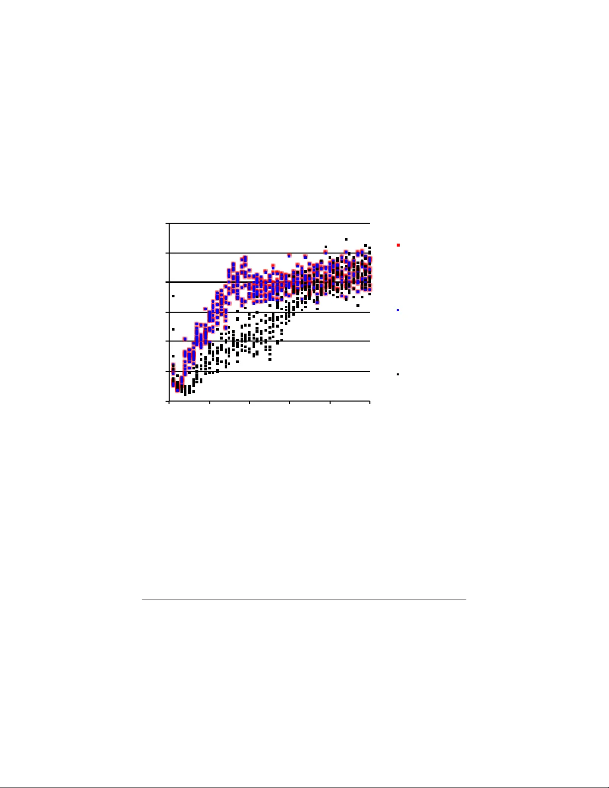
P o or starting p oin ts in mac hine learning Mark T ygert F aceb ook Artificial Intelligence Researc h 1 F aceb ook W ay , Menlo P ark, CA 94025 t ygert@fb.com or tygert@a y a.y ale.edu Septem b er 24, 2018 Abstract P o or (ev en random) starting p oin ts for learning/training/optimization are common in mac hine learning. In man y settings, the metho d of Robbins and Monro (online sto c hastic gradien t descent) is kno wn to b e optimal for goo d starting p oin ts, but may not b e optimal for p o or starting points — indeed, for p oor starting p oints Nesterov acceleration can help during the initial iterations, ev en though Nesterov metho ds not designed for sto c hastic approximation could h urt during later iterations. A go od option is to roll off Nestero v acceleration for later iterations. The common practice of training with nontrivial minibatches enhances the adv an tage of Nesterov acceleration. 1 In tro duction The sc heme of Robbins and Monro (online stochastic gradien t descen t) has long been kno wn to be optimal for sto c hastic approximation/optimization . . . pro vided that the starting p oin t for the iterations is go o d. Y et p o or starting p oin ts are common in mac hine learning, so higher-order metho ds (suc h as Nesterov acceleration) ma y help during the early iterations (ev en though higher-order methods generally hurt during later iterations), as explained b elo w. Belo w, w e elab orate on Section 2 of Sutsk ever et al. (2013), giving some more rigorous mathematical details, somewhat similar to those given by D´ efossez and Bac h (2015) and Flammarion and Bach (2015). In particular, we discuss the key role of the noise level of estimates of the ob jectiv e function, and stress that a large minibatch size mak es higher- order metho ds more effectiv e for more iterations. Our presentation is purely exp ository; w e disav o w an y claim we might mak e to originalit y — in fact, our observ ations should be ob vious to experts in sto c hastic appro ximation. W e opt for concision o ver full mathematical rigor, and assume that the reader is familiar with the sub jects reviewed b y Bach (2013). The remainder of the presen t pap er has the following structure: Section 2 sets math- ematical notation for the s tochastic appro ximation/optimization considered in the sequel. Section 3 elab orates a principle for accelerating the optimization. Section 4 discusses mini- batc hing. Section 5 supplemen ts the n umerical examples of Bac h (2013) and Sutsk ever et al. (2013). Section 6 reiterates the ab o ve, concluding the pap er. 1 2 A mathematical form ulation Mac hine learning commonly inv olves a cost/loss function c and a single random sample X of test data; we then w ant to select parameters θ minimizing the exp ected v alue e ( θ ) = E [ c ( θ, X )] (1) ( e is kno wn as the “error” or “risk” — specifically , the “test” error, as opp osed to “training” error). The cost c is generally a nonnegative scalar-v alued function, whereas θ and X can b e vectors of real or complex n umbers. In sup ervised learning, X is a vector which con tains b oth “input” or “feature” entries and corresp onding “output” or “target” entries — for example, for a regression the input entries can b e regressors and the outputs can b e regressands; for a classification the outputs can b e the lab els of the correct classes. F or training, we hav e no access to X (nor to e ) directly , but can only access indep endent and iden tically distributed (i.i.d.) samples from the probabilit y distribution p from whic h X arises. Of course, e ( θ ) dep ends only on p , not on an y particular sample dra wn from p . T o finish setting our notational con ven tions, we define the deviation or disp ersion d ( θ , X ) = c ( θ , X ) − e ( θ ) , (2) yielding the decomp osition c ( θ , X ) = e ( θ ) + d ( θ , X ) . (3) Com bining (2) and (1) yields that E [ d ( θ , X )] = 0 (4) for all θ , that is, the mean of d ( θ , X ) is 0 (whereas the mean of c ( θ , X ) is e ( θ )). 3 Accelerated learning F or definiteness, w e limit consideration to algorithms whic h ma y access only v alues of c ( θ , x ) and its first-order deriv atives/gradien t with respect to θ . W e assume that the cost c is calibrated (shifted by an appropriate constan t) suc h that the absolute magnitude of c is a go od absolute gauge of the quality of θ (low er cost is b etter, of course). As reviewed, for example, by Bac h (2013), the algorithm of Robbins and Monro (online sto chastic gradien t descen t) minimizes the test error e in (1) using a num b er of samples (from the probabilit y distribution p ) that is optimal — optimal to within a constant factor whic h dep ends on the starting point for θ . Despite this kind of optimality , if e happ ens to start muc h larger than d = c − e , then a higher-order metho d (such as the Nestero v acceleration discussed by Bach (2013) and others) can dramatically reduce the constan t. W e sa y that θ is “p o or” to mean that e ( θ ) is m uch larger than d ( θ , X ). If θ is p o or, that is, e ( θ )  | d ( θ , X ) | , (5) then (3) yields that c ( θ , X ) = e ( θ ) + d ( θ , X ) ≈ e ( θ ) (6) 2 is effectively deterministic, and so Nesterov and other metho ds from Bach (2013) could accelerate the optimization until the up dated θ is no longer p o or. Clearly , θ b eing p o or, that is, e ( θ ) b eing muc h larger than d ( θ , X ), simply means that c ( θ , x ) = e ( θ ) + d ( θ , x ) dep ends mostly just on the probability distribution p underlying X , but not so m uch on an y particular sample x from p . (F or supervised learning, th e probabilit y distribution p is join t ov er the inputs and outputs, enco ding the relation b et w een the inputs and their respective outputs.) If θ is p o or, that is, e ( θ ) is m uc h larger than d ( θ, X ), so that c ( θ , X ) ≈ e ( θ ) is mostly deterministic, then Nesterov methods can be helpful. Of course, optimization p erformance ma y suffer from applying a higher-order metho d to a rough, random ob jectiv e (say , to a random v ariable c ( θ , X ) estimating e ( θ ) when the standard deviation of c ( θ , X ) is high relativ e to e ( θ )). F or instance, Nestero v metho ds essen tially sum across several iterations; if the v alues b eing summed w ere sto c hastically indep enden t, then the summation w ould actually increase the v ariance. In ac c or danc e with the optimality of the metho d of R obbins and Monr o (online sto chastic gr adient desc ent), Nester ov ac c eler ation c an b e effe ctive only when the estimates of the obje ctive function ar e dominantly deterministic, with the obje ctive function b eing the test err or e fr om (1). In practice, we can apply higher-order methods during the initial iterations when the starting p oin t is po or, gradually transitioning to the original metho d of Robbins and Monro (sto c hastic gradient descen t) as the test error approaches its low er limit, that is, as sto c hastic v ariations in estimates of the ob jectiv e function and its deriv atives become imp ortant. 4 Minibatc hes Some practical considerations detailed, for example, b y LeCun et al. (1998) are the follo wing: Man y mo dern micropro cessor arc hitectures can lev erage the parallelism inherent in batc h pro cessing. With suc h parallel (and partly parallel) pro cessors, minimizing the n umber of samples drawn from the probability distribution underlying the data may not b e the most efficient p ossibilit y . Rather than up dating the parameters b eing learned for random individual samples as in online stochastic gradient descen t, the common curren t practice is to draw all at once a num b er of samples — a collection of samples known as a “minibatc h” — and then up date the parameters sim ultaneously for all these samples b efore pro ceeding to the next minibatch. With sufficient parallelism, pro cessing an entire minibatc h may tak e little longer than pro cessing a single sample. Av eraging the estimates of the ob jective function (that is, of the test error e ) and its deriv atives o ver all samples in a minibatch yields estimates with smaller standard deviations, effectiv ely making more parameter v alues b e “po or,” so that Nesterov acceleration is more effectiv e for more iterations. Moreov er, minibatches pro vide (essen tially for free) estimates of the standard deviations of the estimates of e . The num b er of initial iterations for which Nestero v metho ds can accelerate the optimization can b e made arbitrarily large by setting the size of the minibatches arbitrarily large. That said, smaller minibatch sizes t ypically require fewer samples in total to approac h full con vergence (albeit t ypically with more iterations, pro cessing one minibatch p er iteration). Also, after sufficien tly many iterations, sto c hastic v ariations in estimates of the ob jective function and its deriv atives can b ecome imp ortan t, and contin uing to use Nesterov acceleration in these later iterations would b e coun terpro ductiv e. Again, w e recommend applying higher-order metho ds during the initial 3 iterations when the starting p oin t is p o or, noting that larger minibatc hes mak e the higher- order metho ds adv antageous for more iterations b efore the p oin t requiring turning off the Nestero v acceleration. 5 Numerical exp erimen ts The present section supplemen ts the examples of Bach (2013) and Sutskev er et al. (2013) with a few more exp erimen ts indicating that a higher-order metho d — namely , momen tum, a form of Nestero v acceleration — can help a bit in training conv olutional net works. All training rep orted is via the metho d of Robbins and Monro (sto c hastic gradien t descent), with minibatc hes first of size 1 sample p er iteration (as in the original, online algorithm) and then of size 100 samples p er iteration (size 100 is among the most common c hoices used in practice on modern pro cessors which can lev erage the parallelism inherent in batch pro cessing). Section 4 and the third-to-last paragraph of the presen t section describ e the minibatc hing in more detail. Figures 1 and 3 report the accuracies for v arious configurations of “momentum” and “learning rates”; momentum appears to accelerate training somewhat, esp ecially with the larger size of minibatches. Eac h iteration subtracts from the parameters being learned a m ultiple of a stored v ector, where the m ultiple is the “learning rate,” and the stored v ector is the estimated gradien t plus the stored vector from the previous iteration, with the latter stored v ector scaled by the amount of “momen tum”: θ ( i ) = θ ( i − 1) − α ( i ) l . r . v ( i ) , (7) with v ( i ) = β ( i ) mom . v ( i − 1) + 1 k k X j =1  ∂ c ∂ θ  θ , x ( i,j )       θ = θ ( i − 1) , (8) where i is the index of the iteration, θ ( i ) is the up dated vector of parameters, θ ( i − 1) is the previous vector of parameters, v ( i ) is the up dated stored auxiliary vector, v ( i − 1) is the previous stored auxiliary vector, α ( i ) l . r . is the learning rate, β ( i ) mom . is the amount of momen tum, x ( i,j ) is the j th training sample in the i th minibatch, k is the size of the minibatch, and ∂ c/∂ θ is the gradient of the cost c with resp ect to the parameters θ . F ollowing LeCun et al. (1998) exactly as done b y Chintala et al. (2015), the arc hitecture for generating the feature activ ations is a con volutional net work (convnet) consisting of a series of stages, with eac h stage feeding its output in to the next. The last stage has the form of a multinomial logistic regression, applying a linear transformation to its inputs, follo w ed b y the “softmax” detailed by LeCun et al. (1998), thus pro ducing a probability distribution o ver the classes in the classification. The cost/loss is the negativ e of the natural logarithm of the probability so assigned to the correct class. Each stage b efore the last conv olves eac h image from its input against sev eral learned conv olutional k ernels, summing together the con volv ed images from all the inputs into sev eral output images, then takes the absolute v alue of eac h pixel of eac h resulting image, and finally av erages o ver each patch in a partition of each image into a grid of 2 × 2 patches. All conv olutions are complex v alued and pro duce pixels only where the original images cov er all necessary inputs (that is, a conv olution reduces each dimension of the image by one less than the size of the conv olutional k ernel). 4 W e subtract the mean of the pixel v alues from each input image b efore pro cessing with the con vnet, and w e app end an additional feature activ ation feeding into the “softmax” to those obtained from the convnet, namely the standard deviation of the set of v alues of the pixels in the image. The data is a subset of the 2012 ImageNet set of Russak ovsky et al. (2015), retaining 10 classes of images, representing eac h class by 100 samples in a training set and 50 p er class in a testing set. Restricting to this subset facilitated more extensive exp erimen tation (optimizing h yp erparameters more extensiv ely , for example). The images are full color, with three color channels. W e neither augmen ted the input data nor regularized the cost/loss functions. W e used the T orch7 platform — h ttp://torch.c h — for all com putations. T able 1 details the convnet architecture we tested. “Stage” sp ecifies the p ositions of the indicated la yers in the con vnet. “Input channels” specifies the num b er of images input to the giv en stage for each sample from the data. “Output channels” sp ecifies the num b er of images output from the given stage. Each input image is conv olved against a separate, learned con volutional k ernel for each output image (with the results of all these con vol utions summed together for each output image). “Kernel size” sp ecifies the size of the square grid of pixels used in the conv olutions. “Input c hannel size” sp ecifies the size of the square grid of pixels constituting each input image. “Output channel size” sp ecifies the size of the square grid of pixels constituting eac h output image. The feature activ ations that the con vnet pro duces feed into a linear transformation follow ed by a “softmax,” as detailed b y LeCun et al. (1998). F or the minibatch size 100, rather than up dating the parameters b eing learned for randomly selected individual images from the training set as in online sto c hastic gradient descen t, w e instead do the following: we randomly p erm ute the training set and partition this p erm uted set of images into subsets of 100, up dating the parameters simultaneously for all 100 images constituting eac h of the subsets (known as “minibatches”), pro cessing the series of minibatc hes in series. Each sweep through the entire training set is kno wn as an “ep och.” LeCun et al. (1998), among others, made the ab o v e terminology the standard for training convnets. The horizontal axes in the figures count the n umber of epo chs. Figures 1 and 2 presen t the results for minibatches of size 100 samples p er iteration; Figure 3 presen ts the results for minibatches of size 1 sample p er iteration. “Av erage precision” is the fraction of all classifications which are correct, c ho osing only one class for eac h input sample image from the test set. “Error on the test set” is the av erage o ver all samples in the test set of the negative of the natural logarithm of the probabilit y assigned to the correct class (assigned by the “softmax”). “Co efficien t of v ariation” is an estimate of the standard deviation of c ( θ , X ) (from (1)) divided b y the mean of c ( θ , X ), that is, an estimate of the standard deviation of d ( θ, X ) (from (2)) divided b y e ( θ ) (from (1) and (2)). Rolling off momentum as the co efficien t of v ariation increases can b e a go od idea. Please b ew are that these exp erimen ts are far from definitiv e, and ev en here the gains from using momentum seem to b e marginal. Even so, as Section 4 discusses, minibatching effectiv ely reduces the standard deviations of estimates of the ob jective function e , making Nestero v acceleration more effectiv e for more iterations. 5 6 Conclusion Though in many settings the metho d of Robbins and Monro (sto c hastic gradient descen t) is optimal for go od starting p oin ts, higher-order metho ds (suc h as momentum and Nestero v acceleration) can help during early iterations of the optimization when the parameters b eing optimized are p o or in the sense discussed ab ov e. The opportunity for accelerating the optimization is clear theoretically and apparen tly observ able via n umerical experiments. Minibatc hing makes the higher-order methods adv antageous for more iterations. That said, higher order and higher accuracy need not b e the same, as higher order guarantees only that accuracy increase at a faster rate — higher order guaran tees higher accuracy only after enough iterations. Ac kno wledgemen ts W e would like to thank F rancis Bach, L´ eon Bottou, Y ann Dauphin, Piotr Doll´ ar, Y ann LeCun, Marc’Aurelio Ranzato, Arthur Szlam, and Rac hel W ard. A A simple analytical example This app endix w orks through a v ery simple one-dimensional example. Consider the cost c as a function of a real scalar parameter θ and sample of data x , defined via c ( θ , x ) = ( θ − x ) 2 . (9) Supp ose that X is the (Rademac her) random v ariable taking the v alue 1 with probabilit y 1 / 2 and the v alue − 1 with probabilit y 1 / 2. Then, the co efficien t of v ariation of c ( θ , X ), that is, the standard deviation σ ( θ ) of c ( θ , X ) divided by the mean e ( θ ) of c ( θ, X ), is σ ( θ ) e ( θ ) = 2 | θ | θ 2 + 1 : (10) (pr o of ) X taking the v alue 1 with probability 1 / 2 and the v alue − 1 with probabilit y 1 / 2 yields that | X | = 1 (11) and that the exp ected v alue of X is 0, E [ X ] = 0 . (12) Com bining (9) and (11) then yields c ( θ , X ) = θ 2 + 1 − 2 θ X . (13) Moreo ver, together with the definitions (1) and (2), com bining (13) and (12) yields e ( θ ) = E [ c ( θ, X )] = θ 2 + 1 (14) 6 and d ( θ , X ) = c ( θ, X ) − e ( θ ) = − 2 θX . (15) The mean of c ( θ , X ) is this e ( θ ) in (14). The standard deviation of c ( θ , X ) is the same as the standard deviation of d ( θ , X ) in (15), whic h is just σ ( θ ) = 2 | θ | , (16) due to (15) combined with X taking the v alue 1 with probability 1 / 2 and the v alue − 1 with probabilit y 1 / 2. Com bining (14) and (16) yields (10), as desired.  The secant method (a higher-order metho d) consists of the iterations up dating θ ( i − 2) and θ ( i − 1) to θ ( i ) via θ ( i ) = θ ( i − 1) − ∂ c ∂ θ  θ ( i − 1) , x ( i − 1)  ·  θ ( i − 1) − θ ( i − 2)    ∂ c ∂ θ  θ ( i − 1) , x ( i − 1)  − ∂ c ∂ θ  θ ( i − 2) , x ( i − 2)   , (17) where x ( i − 2) , x ( i − 1) , and x ( i ) are independent realizations (random samples) of X and the deriv ative of c ( θ, x ) from (9) with resp ect to θ is ∂ c ∂ θ = 2( θ − x ); (18) com bining (17) and (18) and simplifying yields θ ( i ) =  θ ( i − 1) x ( i − 2) − θ ( i − 2) x ( i − 1)    θ ( i − 1) − x ( i − 1) − θ ( i − 2) + x ( i − 2)  . (19) In the limit that b oth x ( i − 1) and x ( i − 2) b e 0, (19) shows that θ ( i ) is also 0 (pro vided that θ ( i − 1) and θ ( i − 2) are distinct), that is, the secan t metho d finds the optimal v alue for θ in a single iteration in such a limit. In fact, (14) mak es clear that the optimal v alue for θ is 0, while combining (19) and (11) yields that | θ ( i ) | ≤  | θ ( i − 1) | + | θ ( i − 2) |    | θ ( i − 1) − θ ( i − 2) | − 2  , (20) so that | θ ( i ) | is likely to b e reasonably small (around 1 or so) even if | θ ( i − 1) | or | θ ( i − 2) | (or b oth) are v ery large and random and | X | = 1. Ho wev er, these iterations generally fail to con v erge to any v alue muc h s maller than unit magnitude: with probability 1 / 2, indeed, x ( i − 2) = x ( i − 1) = 1 or x ( i − 2) = x ( i − 1) = − 1; hence (19) yields that | θ ( i ) | = 1 with probability at least 1 / 2, assuming that θ ( i − 2) and θ ( i − 1) are distinct (while in the degenerate case that θ ( i − 2) and θ ( i − 1) tak e exactly the same v alue, θ ( i ) also takes that same v alue). All in all, a sensible strategy is to start with a higher-order method (such as the secant metho d) when | θ | is large, and transition to the asymptotically optimal method of Robbins and Monro (sto c hastic gradien t descent) as | θ | b ecomes of roughly unit magnitude. The transition can b e based on | θ | or on estimates of the co efficien t of v ariation — due to (10), the co efficien t of v ariation is essentially in v ersely prop ortional to | θ | when | θ | is large. 7 Figure 1: T est accuracies for v arious settings of momen tum (mom.) and learning rates (l.r.) [minibatc h size 100] (a) 0" 0.1" 0.2" 0.3" 0.4" 0.5" 0.6" 0" 10" 20" 30" 40" 50" average&precision& epoch& higher&average-precision&is&be0er& mom.=.9,"l.r.=8," when"epoch<20;" mom.=0,"l.r.=.02," otherwise" mom.=.9,"l.r.=8," when"epoch<20;" mom.=.9,"l.r.=.02," otherwise" mom.=0,"l.r.=3," when"epoch<30;" mom.=0,"l.r.=.9," otherwise" (b) 0" 0.5" 1" 1.5" 2" 2.5" 0" 10" 20" 30" 40" 50" error$on$the$test$set$ epoch$ lower$error$on$the$test$set$is$be/er$ mom.=.9,"l.r.=8," when"epoch<20;" mom.=0,"l.r.=.02," otherwise" mom.=.9,"l.r.=8," when"epoch<20;" mom.=.9,"l.r.=.02," otherwise" mom.=0,"l.r.=3," when"epoch<30;" mom.=0,"l.r.=.9," otherwise" 8 Figure 2: Estimated co efficien ts of v ariation (CVs) of the cost c ( θ , X ) in (1) and (3), using all samples in eac h minibatch to construct estimates of the CVs (the estimates of the CVs are themselves sub ject to sto c hastic v ariations; the distribution of the plotted p oints within an ep o c h provides an indication of the probabilit y distribution of the estimates of the CVs) [minibatc h size 100] 0" 0.2" 0.4" 0.6" 0.8" 1" 1.2" 0" 10" 20" 30" 40" 50" coefficient(of(varia-on(of(the(cost ( ( c ( θ , # X ) ( —(the(cost's(std.(dev.(divided(by(its(mean( epoch( mom.=.9,"l.r.=8," when"epoch<20;" mom.=0,"l.r.=.02," otherwise" mom.=.9,"l.r.=8," when"epoch<20;" mom.=.9,"l.r.=.02," otherwise" mom.=0,"l.r.=3," when"epoch<30;" mom.=0,"l.r.=.9," otherwise" T able 1: Architecture of the conv olutional netw ork input output k ernel input output stage c hannels c hannels size c hannel size c hannel size first 3 16 5 × 5 128 × 128 62 × 62 second 16 64 3 × 3 62 × 62 30 × 30 third 64 256 3 × 3 30 × 30 14 × 14 fourth 256 256 3 × 3 14 × 14 6 × 6 9 Figure 3: T est accuracies for v arious settings of momen tum (mom.) and learning rates (l.r.) [minibatc h size 1] (a) 0" 0.1" 0.2" 0.3" 0.4" 0.5" 0.6" 0" 5" 10" 15" 20" average&precision& epoch& higher&average-precision&is&be0er& mom.=.6,"l.r.=.002," when"epoch<8;" mom.=0,"l.r.=.0002," otherwise" mom.=.6,"l.r.=.002," when"epoch<8;" mom.=.6,"l.r.=.0002," otherwise" mom.=0,"l.r.=.002," when"epoch<10;" mom.=0,"l.r.=.0002," otherwise" (b) 0" 0.5" 1" 1.5" 2" 2.5" 0" 5" 10" 15" 20" error$on$the$test$set$ epoch$ lower$error$on$the$test$set$is$be/er$ mom.=.6,"l.r.=.002," when"epoch<8;" mom.=0,"l.r.=.0002," otherwise" mom.=.6,"l.r.=.002," when"epoch<8;" mom.=.6,"l.r.=.0002," otherwise" mom.=0,"l.r.=.002," when"epoch<10;" mom.=0,"l.r.=.0002," otherwise" 10 References Bac h, F. (2013). Sto c hastic gradient metho ds for machine learning. T ec hnical rep ort, INRIA-ENS, Paris, F rance. http://www.di.ens.fr/ ~ fbach/fbach_sgd_online.pdf . Chin tala, S., Ranzato, M., Szlam, A., Tian, Y., T ygert, M., and Zarem ba, W. (2015). Scale-in v arian t learning and con volutional netw orks. T echnical Rep ort 1506.08230, arXiv. http://arxiv.org/abs/1506.08230 . D ´ efossez, A. and Bach, F. (2015). Av eraged least-mean-squares: bias-v ariance trade-offs and optimal sampling distributions. In Pr o c. 18th Internat. Conf. Artificial Intel ligenc e and Statistics , volume 38, pages 205–213. http://jmlr.org/proceedings/papers/v38/ defossez15.pdf . Flammarion, N. and Bach, F. (2015). F rom av eraging to acceleration, there is only a step- size. T echnical Report 1504.01577, arXiv. . LeCun, Y., Bottou, L., Bengio, Y., and Haffner, P . (1998). Gradien t-based learning ap- plied to do cumen t recognition. Pr o c. IEEE , 86(11):2278–2324. http://yann.lecun. com/exdb/publis/pdf/lecun- 98.pdf . Russak ovsky , O., Deng, J., Su, H., Kruse, J., Satheesh, S., Ma, S., Huang, Z., Karpath y , A., Khosla, A., Bernstein, M., Berg, A. C., and F ei-F ei, L. (2015). ImageNet large scale visual recognition challenge. T echnical Report 1409.0575v3, arXiv. abs/1409.0575 . Sutsk ever, I., Martens, J., Dahl, G., and Hinton, G. (2013). On the imp ortance of ini- tialization and momen tum in deep learning. In Pr o c. 30th International Confer enc e on Machine L e arning , v olume 28, pages 1139–1147. J. Machine Learning Research. http://www.jmlr.org/proceedings/papers/v28/sutskever13.pdf . 11