Machine Learning Model of the Swift/BAT Trigger Algorithm for Long GRB Population Studies

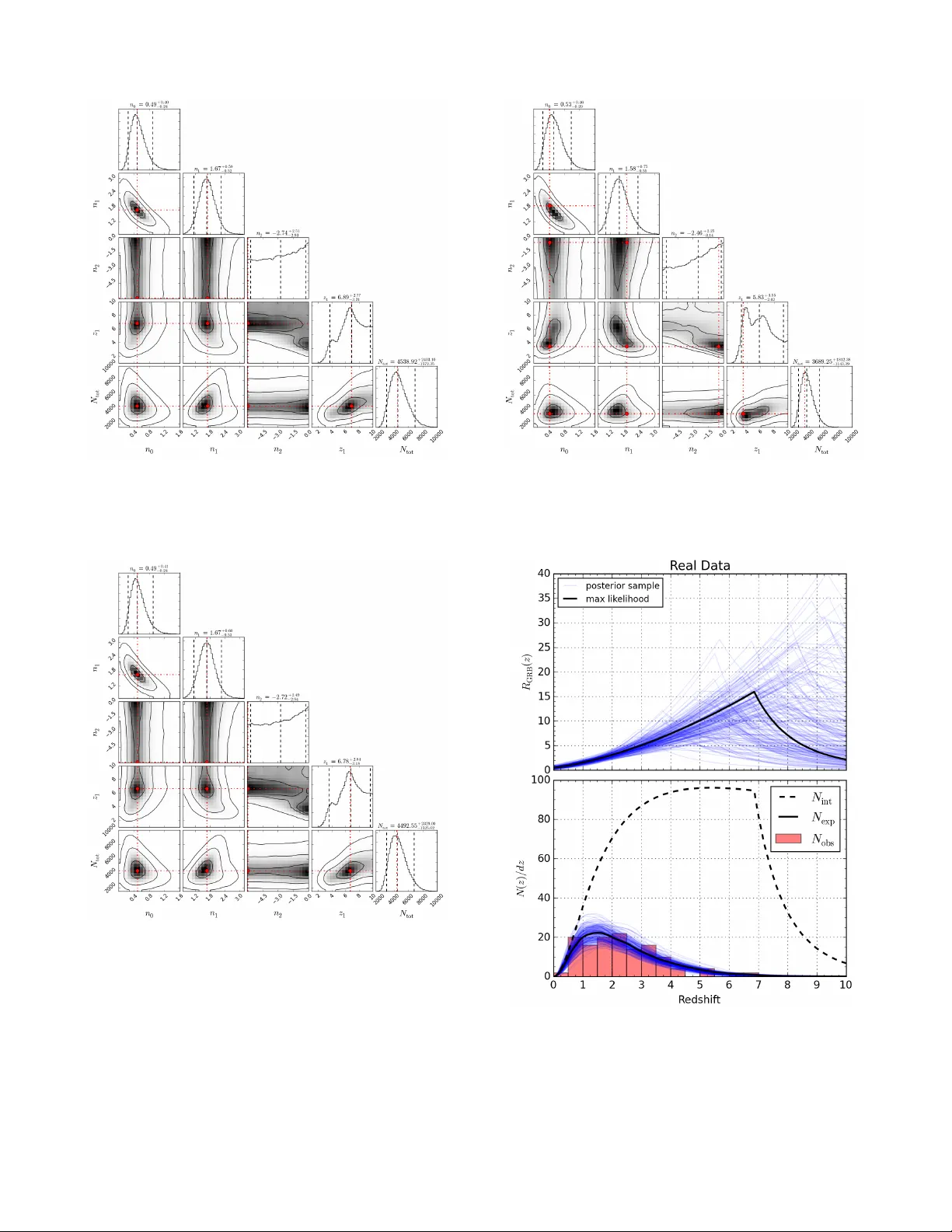
S U B M I T T E D T O A P J Preprint typeset using L A T E X style emulateapj v . 01/23/15 MA CHINE LEARNING MODEL OF THE SWIFT/B A T TRIGGER ALGORITHM FOR LONG GRB POPULA TION STUDIES P H I L I P B . G R A FF Department of Physics and Joint Space Science Institute, Univ ersity of Maryland, College Park, MD 20742, USA and N ASA Goddard Space Flight Center, 8800 Greenbelt Rd., Greenbelt, MD 20771, USA A M Y Y . L I E N N ASA Goddard Space Flight Center, 8800 Greenbelt Rd., Greenbelt, MD 20771, USA J O H N G . B A K E R N ASA Goddard Space Flight Center, 8800 Greenbelt Rd., Greenbelt, MD 20771, USA T A K A N O R I S A K A M O TO Department of Physics and Mathematics, College of Science and Engineering, Aoyama Gakuin Uni versity , 5-10-1 Fuchinobe, Chuo-ku, Sagamihara-shi, Kanagawa 252-5258, Japan Submitted to ApJ ABSTRA CT T o draw inferences about gamma-ray burst (GRB) source populations based on Swift observations, it is es- sential to understand the detection efﬁcienc y of the Swift burst alert telescope (BA T). This study considers the problem of modeling the Swift /B A T triggering algorithm for long GRBs, a computationally expensiv e proce- dure, and models it using machine learning algorithms. A lar ge sample of simulated GRBs from Lien et al. ( 2014 ) is used to train v arious models: random forests, boosted decision trees (with AdaBoost), support v ector machines, and artiﬁcial neural networks. The best models have accuracies of & 97% ( . 3% error), which is a signiﬁcant improvement on a cut in GRB ﬂux which has an accuracy of 89 . 6% ( 10 . 4% error). These models are then used to measure the detection efﬁciency of Swift as a function of redshift z , which is used to perform Bayesian parameter estimation on the GRB rate distribution. W e ﬁnd a local GRB rate density of n 0 ∼ 0 . 48 +0 . 41 − 0 . 23 Gp c − 3 yr − 1 with po wer-la w indices of n 1 ∼ 1 . 7 +0 . 6 − 0 . 5 and n 2 ∼ − 5 . 9 +5 . 7 − 0 . 1 for GRBs above and below a break point of z 1 ∼ 6 . 8 +2 . 8 − 3 . 2 . This methodology is able to impro ve upon earlier studies by more accurately modeling Swift detection and using this for fully Bayesian model ﬁtting. The code used in this is analysis is publicly av ailable online a . K eywor ds: gamma rays: general, methods: data analysis 1. INTR ODUCTION Long gamma-ray b ursts (GRBs) are related to core-collapse supernov ae from the death of massive stars. These are im- portant for studying star-formation history , particularly in the early universe where other methods become difﬁcult. The Swift space telescope ( Gehrels et al. 2004 ) is able to detect and localize these out to large distances and quickly do wnlink the data to the ground. These abilities enable prompt ground- based followup observations that can provide redshift mea- surements of the GRBs. T o date, Swift has detected over 900 GRBs, of which ∼ 30% hav e redshift measurements. From these observations, one can try to infer the intrinsic GRB rate that is connected to stellar ev olution over the history of the Univ erse. Many researchers have used Swift ’ s observ ations to study intrinsic GRB redshift and luminosity distrib utions, and the implications for star-formation history (e.g., Guetta and Della V alle 2007 ; Guetta and Piran 2007 ; Y ¨ uksel et al. 2008 ; Kistler et al. 2008 ; Butler et al. 2010 ; Robertson and Ellis 2012 ; P ´ elangeon et al. 2008 ; Salvaterra et al. 2009 ; Campisi et al. 2010 ; W anderman and Piran 2010 ; V ir gili et al. 2011 ; pgraff@umd.edu amy .y .lien@nasa.gov john.g.baker@nasa.gov a https://github.com/PBGraff/SwiftGRB_PEanalysis Qin et al. 2010 ; Salvaterra et al. 2012 ; Cow ard et al. 2013 ; Kanaan and de Freitas Pacheco 2013 ; W ang 2013 ; Lien et al. 2014 ; Howell et al. 2014 ; Y u et al. 2015 ; Petrosian et al. 2015 ; Pescalli et al. 2015 ). Sev eral studies have suggested that the GRB rate at high redshift ( z & 5 ) is larger than the expectation based on star-formation rate (SFR) measurements (e.g., Le and Der- mer 2007 ; Y ¨ uksel et al. 2008 ; Kistler et al. 2009 ; Butler et al. 2010 ; Ishida et al. 2011 ; T an vir et al. 2012 ; Jakobsson et al. 2012 ; Lien et al. 2014 ). This result could imply sev eral pos- sibilites, such as a larger star-formation rate in the early uni- verse(e.g., Kistler et al. 2009 ; T an vir et al. 2012 ), an ev olv- ing luminosity function(e.g., V ir gili et al. 2011 ; Pescalli et al. 2015 ), or a different GRB to supernova ratio (i.e. a different scenario of stellar e volution) due to a different en vironment in the early univ erse (e.g., W oosley and Heger 2012 ). Howe ver , it remains difﬁcult to constrain the GRB rate. Though Swift has observed a lar ge population of GRBs only some of these ha ve measured redshifts. Even with a relati vely complete redshift sub-sample, there are complicated selec- tion effects from the complex trigger algorithm adopted by the burst alert telescope (B A T) on-board Swift and the difﬁ- culty in searching through a large parameter space. It is chal- lenging to distinguish the luminosity function and the redshift 2 distribution using the observational data. W e address some of these issues with a machine learning approach to produce a fast, but reliable, treatment of Swift ’ s instrumental selection effects, thereby enabling a robust Bayesian treatment of pop- ulation model analysis. Machine learning (ML) is a ﬁeld of research that inv olves designing algorithms (MLAs) for building models that learn from generic data. The models are ﬁt to a set of training data in order to make predictions or decisions. Often, the original training data come from actual observations or simulations of a complex process. The models trained by MLAs can be ev aluated very quickly for any new example after a one-time cost of training the model. In this study , we look to aid the analysis of GRB data by using MLAs to train models that emulate the Swift trigger al- gorithm. Our training data comes from simulations of GRB populations computed by Lien et al. ( 2014 ). The structure of this paper is as follows. In Section 2 we de- scribe the aspects of Swift and its model for triggering on in- cident GRBs that are relev ant to GRB population inferences. Then, in Section 3 we describe the machine learning algo- rithms used and compared in this study . Section 4 presents the results of training the dif ferent ML models on the training data from the Swift pipeline. W e apply a trained ML model for accelerating Bayesian inference with faster likelihoods in Section 5 , ﬁtting the parameters of the intrinsic GRB rate dis- tribution. Section 6 compares our study to pre vious work es- timating the intrinsic distributions of long GRBs with Swift observations. Lastly , in Sections 7 and 8 we summarize and propose future projects to follow-up. 2. THE Swift DETECTION ALGORITHM The b urst alert telescope (B A T) on-board Swift adopts o ver 500 rate trigger criteria based on photon count rate in the raw light curv e. Moreo ver , the burst needs to pass the “im- age threshold” determined by the signal-to-noise ratio esti- mated from an image generated on-board based on the dura- tion found by the rate trigger criteria. Each rate trigger crite- rion uses a dif ferent ener gy band, dif ferent part of the detector plane, and different fore ground and background durations for calculating the signal-to-noise ratio. In addition to the rate trigger algorithm, the BA T also generates an image e very & minute to search for bursts that are missed by the rate trigger method (which is the so-called “image trigger”) ( Barthelmy et al. 2005 ; Fenimore et al. 2003 , 2004 ; McLean et al. 2004 ; Palmer et al. 2004 ). This complex trigger algorithm successfully increases the number of GRB detections. Howe ver , it also increases the dif- ﬁculty of estimating the detection theshold, which is curcial for probing many intrinsic GRB properties from the observa- tions. T o address this problem, Lien et al. ( 2014 ) de veloped a code that simulates the B A T trigger algorithm, and used it to study the instrinsic GRB rate and luminosity function. This “trigger simulator” follo ws the same trigger algorithm and cri- teria for the rate trigger as those adopted by the B A T , and mimics the image threshold and image trigger (see Lien et al. ( 2014 ) for detailed descriptions). Although the trigger simu- lator can be used to address the complex detection thresholds of the B A T , it takes ∼ 10 seconds to a few minutes to simulate the trigger status of a burst using a common PC with the 2.7 GHz Intel Core processor (the speed mainly depends on the number of bins in the light curve). Therefore, it is computa- tionally intensi ve to perform a lar ge number of simulations to cov er a wide parameter space. This is where machine learning is able to accelerate our analysis. 3. MACHINE LEARNING ALGORITHMS T o generate a fast emulator for the Swift trigger simula- tor , we consider a v ariety of supervised learning algorithms, where the goal is to infer a function from labeled training data. Each example consists of input properties which are used to predict the output label. Here we brieﬂy describe each of the machine learning algo- rithms used in this study . W e denote the set of input features by x and the machine learning model’ s predicted output is giv en by y ( x ) . The inputs are a set of 15 parameters describ- ing the GRB and detector as detailed in T able 1 . Depending on the MLA, the output may be a discrete label, e.g. { 0 , 1 } , or it may be a continuous probability in [0 , 1] and is designed to be the probability that a GRB, as speciﬁed by the features in x , is detected by Swift ’ s B A T . The true output is giv en by t and is 0 for a non-detection and 1 for a detection. 3.1. Random F or ests and AdaBoost Random forests and AdaBoost both inv olve creating en- sembles of decision trees, so we ﬁrst introduce these as a ma- chine learning model. In a decision tree, binary splits are per- formed on the training data input features, the dimensions of x . In training a tree on data, a series of splits are made that choose a dimension and a threshold that optimize some crite- rion. Examples of this criterion are the accuracy of the result- ing classiﬁcations (maximize; equiv alently minimize errors) or the Gini impurity (minimize) which giv en by G = 1 − X i = { 0 , 1 } f 2 i , (1) where f i is the fraction of correctly classiﬁed samples labeled with value i . This measure aims to make each sub-set result- ing from a branch as “pure” as possible in the class labels of its members. Each split creates a pair of “branches”, one with each class label. These splits are made until a stopping con- dition is reached (e.g. the samples are all of uniform class, a maximum number of splits has been reached, or the num- ber of samples left to split among has fallen below a mini- mum v alue). This branch now becomes a “leaf ” that assigns a class to all samples ending there. When a new event of un- known class is put into the tree, the tree will pass it through the learned splits/branches until it reaches a leaf, at which point it will be labeled according to the label of the leaf. An example tree ﬁt to this data (with a hard limit of 3 in depth) is sho wn in Figure 1 ; it has a classiﬁcation accurac y of 93 . 9% on the training data to which it was ﬁt. T rees ﬁt in the later models will be much larger and thus more accurate. 3.1.1. Random F orests Random forests (RFs) ( Breiman 2001 ) improve upon clas- sical decision trees by training an ensemble of trees that vote on the ﬁnal classiﬁcation. A “strong learner” (the RF) is cre- ated from an ensemble of “weak learners” (decision trees). In a RF , many decision trees are trained on the data – often hundreds. T o obtain many different trees, at each split in a tree, a random subset of the dimensions of x are chosen and the optimal binary split to be made out of these dimensions is made. Furthermore, each tree is trained on a bootstrap sample of the data; the original K points are sampled with replace- ment to form a new set of K points that may contain repeats. A RF thus guards against overﬁtting to the training data and 3 Figure 1. A decision tree ﬁt to the Swift training data with a maximum depth of 3 . An accuracy of 93 . 9% is achiev ed. Each box shows the parameter chosen for branching and the threshold used, as well as the total number of samples used to make that decision. The Gini factor shown is that from Equation ( 1 ) for the subset at that location. At the leaves, the number of items with class 0 and class 1 are shown; the tree can assign class probabilities based on this split at the leaf that any ne w sample arrives at after follo wing the branches down. potentially badly performing individual trees. A single tree can provide a probabilistic classiﬁcation, y DT ( x ) ∈ [0 , 1] , and combining many allows us to obtain a near-continuous probability , y RF ( x ) ∈ [0 , 1] by using y RF ( x ) = 1 N N X n =1 y DT ,n ( x ) , (2) with N being the number of trees in the forest. This value we obtain as y RF ( x ) is simply the probability that the GRB described by x is detected by Swift . W e use the implementation of RFs in the scikit-learn 1 Python library ( Pedregosa et al. 2011 ). 3.1.2. AdaBoost AdaBoost is short for “ Adapti ve Boosting”, a meta- algorithm for machine learning ( Freund and Schapire 1997 ). It creates a single strong learner from an ensemble of weak learners, much like RFs. Ho wev er , in the boosting frame- work, the decision trees are trained iterativ ely and when added together (as in Equation ( 2 )) are weighted, typically based on their accuracy . Additionally , unlike for RFs, the training ex- amples will not be all equally weighted when e valuating the accuracy . After an indi vidual decision tree is added to the en- semble, the training data is reweighed so that examples that are misclassiﬁed increase in weighting and those classiﬁed correctly decrease in weighting. Therefore, future decision trees will attempt to better ﬁt examples previously misclassi- ﬁed. In this w ay , the o verall ensemble prediction may become more accurate. Boosting may be applied to any machine learning algo- rithm, but in this work we apply it only to the decision tree weak learner (the other classiﬁers qualify as strong learners on their own and would thus likely not beneﬁt signiﬁcantly from boosting). W e use the implementation of AdaBoost for decision tree classiﬁers in scikit-learn . W e note that the predicted probability , y AB ( x ) ∈ [0 , 1] , is approximately continuous, similarly to y RF ( x ) . 3.2. Support V ector Machines Support vector machines (SVMs) ( Cortes and V apnik 1995 ) are a tool for binary classiﬁcation that ﬁnds the optimal hyper-plane for separating the two classes of training sam- ples. Events are classiﬁed by which side of the hyper-plane they fall on. The hyper -plane that maximizes the separation 1 http://scikit- learn.org/stable/index.html from points in either class will (in general) have minimal gen- eralization error for new data points. In a linear SVM, we label the two classes with t i ∈ {− 1 , 1 } corresponding to an un-detected GRB and a detected GRB, respectiv ely . A hyper-plane separating the two classes will satisfy w · x − b = 0 , where w and b must be found by training on the data { x } . If the classes are separable, we can place two parallel hyper-planes that separate the points and hav e no points between them in the “margin”. This can be seen for a toy example in Figure 2 . W e describe these hyper- planes mathematically as w · x − b = ± 1 , (3) Examples will lie on either side of the two planes such that t i ( w · x i − b ) ≥ 1 (4) for all samples, x i . As the samples are typically not sepa- rable, we introduce slack variables ξ i ≥ 0 that measure the misclassiﬁcation of x i by setting t i ( w · x i − b ) ≥ 1 − ξ i . (5) W e then seek to minimize Cost ( w , ξ , b ) = 1 2 k w k 2 + C X i ξ i (6) subject to the constraint in Equation 5 . The C parameter is a penalty factor for misclassiﬁcation and this optimization will face the trade-off between a smaller margin and smaller mis- classiﬁcation error . The cost function seeks to maximize the distance between the two hyper-planes at the margin edges, which is giv en by 2 / || w || . This separation by hyper-plane is demonstrated for a toy example in Figure 2 . The two classes of points are generally not easily separated in the original parameter space of the problem. Therefore, we map the points into a higher-dimensional space where they may be more easily separated. T o make this a computation- ally tractable problem, we consider mappings such that the dot product between pairs of points may be easily computed in terms of the original v ariables by a kernel function, k ( x i , x j ) . Hyper-planes in the higher-dimensional space are deﬁned as surfaces on which the kernel is constant. If the kernel is de- ﬁned such that k ( x i , x j ) decreases as the points x i and x j mov e away from one another , then the kernel is a measure of closeness. Thus, the sum of many kernels like this can be used to measure the proximity of a sample data point to data points in the two classes; this distance can then be used to classify the 4 Figure 2. The maximum separating hyper-plane and the mar gin hyper-planes for a toy data set. The “support vectors” are the highlighted points along the margin hyper-planes. Image courtesy of Wikimedia Commons ( Commons 2008 ). point into one class or the other . This mapping can result in a very con v oluted hyper-plane separating the two sets of points – this can accurately model the true classiﬁcation boundary , but we must be careful not to o verﬁt this to the training data. In order to perform a non-linear separation, we employ a Gaussian kernel function (a.k.a. radial basis function), k ( x i , x j ) = exp  − γ k x i − x j k 2  (7) where γ is a tunable parameter reﬂecting the width of the Gaussian. A point is classiﬁed by which side of the learned hyper - plane it falls on, as determined (in our notation) by y ( x ) = sign ( K ( w , x ) − b ) , (8) where K is the aggre gate kernel function that is a linear com- bination of the individual kernel functions (closeness to each of the other points). Minimizing the cost gi ven by Equa- tion ( 6 ) under the constraint of Equation ( 5 ) can be solved as a quadratic programming problem with the solution locally independent of all b ut a few data points, the “support vectors” of the model. These will be those samples closest to or on the margin in both classes and a weighted sum of distances from them will determine which class a ne w sample is in. Points that are not support vectors will have small or zero weight in the aggregate k ernel function. In this study , we use the implementation of SVMs in scikit-learn . A radial basis function is chosen and we perform 5 -fold cross-validation to optimize the hyper- parameters of the model, γ and C . The model is also trained to allow for the prediction of continuous class probabilities, y SVM ∈ [0 , 1] 2 . 3.3. Artiﬁcial Neural Networks Artiﬁcial neural networks are a machine learning method that is inspired by the function of a brain. A neural network (NN) consists of interconnected nodes, each of which pro- cesses information that it receiv es and passes this product on to other nodes via weighted connections. In a feed-forward NN, these nodes are organized into layers that pass informa- tion uniformly in a certain direction. The input layer passes 2 See the scikit-learn documentation for details on this procedure. information to an output layer via zero, one, or many “hid- den” layers in between. Each node in the network performs a simple function, b ut their combined activity can model com- plex relationships. A useful introduction to NNs as well as their training and use can be found in MacKay ( 2003 ). A single node takes an input vector of activ ations a ∈ < N and maps it to a scalar output f ( a ; w , b ) through f ( a ; w , b ) = g b + N X i =1 w i a i ! , (9) where w and b are the parameters of the node, called the “weights” and “bias”, respecti vely . The function, g , is the activ ation function of the node; we use the sigmoid, linear , and rectiﬁed linear activ ation functions in this work. g ( z ) =    (1 + e − z ) − 1 sigmoid z linear max { 0 , z } rectiﬁed linear (10) The sigmoid and rectiﬁed linear activ ations are used for hid- den layer nodes and the linear acti vation is used for the output layer nodes to obtain v alues in ( −∞ , ∞ ) . This is then con- verted into a probability by the softmax transform gi ven by y j ( x ; w , b ) → exp ( y j ( x ; w , b )) P l = { 0 , 1 } exp ( y l ( x ; w , b )) (11) where j indexes over the output nodes. After the softmax, all output values are in (0 , 1) and sum to 1 . W e show here the case where there are only two output nodes for a binary classiﬁcation problem; these values are degenerate, b ut the setup of one output node per class generalizes to the multi- class problem. The weights and biases of all nodes in the network are the parameters that must be optimized with respect to the training data. The number of input nodes is the number of features giv en by the data. The two output nodes are the values in which are the probabilities that the input GRB features would result in detection or non-detection. In this work, we will tak e y NN ( x ) to be the continuous probability given in the output node for the “detection” class. Thus, the output is the pre- dicted probability that the giv en input GRB features corre- spond to a detected GRB. The optimization algorithm seeks to minimize the cross- entropy of the predicted probabilities, gi ven by Cost ( p ) = − X i X k = { 0 , 1 } t i,k log y k ( x i ) (12) where p is a parameter vector containing all of the weights and biases of the nodes in the NN. The index i is over all data samples in the training set and the index k is over the 2 output nodes corresponding to the non-detection and de- tection classes, respecti vely . t i = { 1 , 0 } for a non-detection and t i = { 0 , 1 } for a detection. This cost function pushes predicted probabilities to ward their correct values with large penalties for incorrect predictions and is based in information theory . W e take the v alue from the output node corresponding to the detection class as the probability that the input GRB, x , is detected by Swift , y NN ( x ) . W e use the S K Y N E T 3 algorithm ( Graff et al. 2014 ) for train- ing of the NN and refer the reader to that paper for more in- 3 http://www.mrao.cam.ac.uk/software/skynet/ 5 formation on NNs, including the optimization function used, how the optimization is performed, and additional data pro- cessing that is performed. S K Y N E T provides an easy-to-use interface for training as well as an algorithm that will efﬁ- ciently and consistently ﬁnd the best ﬁt NN parameters for the training data provided. 3.4. Heuristics Used For each model’ s optimal settings, we compute the accu- racy of predictions using a na ¨ ıve probability threshold of 0 . 5 for the output probability for the detection class; i.e. y m ( x ) for the different models, m . This is later found to be close to optimal. W e also plot the receiv er operating characteristic (R OC) curves for the classiﬁers as seen in Figure 9 later . A R OC curve plots the true positive rate (a.k.a. recall) against the false positiv e rate. The F1-score is a useful metric for ﬁnding the optimal probability threshold to balance type I (false positi ve) and type II (false negati ve) errors. The F1- score takes v alues in [0 , 1] and is maximized at the optimal probability threshold. These values are gi ven by: TP = # positives correctly labeled TN = # of negati ves correctly labeled FP = # of negati ves labeled as positiv e FN = # of positives labeled as ne gativ e TPR = TP TP + FN = recall FPR = FP FP + TN precision = TP TP + FP F1-score = 2 precision × recall precision + recall where positiv es are detections and negati ves are non- detections of GRBs. For a random classiﬁer, the R OC will be a diagonal line from (0 , 0) to (1 , 1) . Better classiﬁers will be abov e and to the left of this line. A common measure is the area under the curve (A UC), which is the inte grated area under the R OC. V alues closer to 1 indicate better classiﬁers. In this study , we will use the R OC (with A UC) to ﬁnd the MLA that best models the Swift pipeline. W e can then use the F1-score to identify the best probability threshold for declar- ing a detection from the predictions of the model. 3.5. Cr oss-V alidation T o measure the performance for each type of MLA, we per - form hyper-parameter optimization over a range of settings for each. T o properly compare these settings against each other , we perform cr oss-validation . In this setup, with 5 folds, we split the data into 5 random subsets of equal size. In train- ing, we train 5 models for each setting, using 4 of the 5 dur- ing ﬁtting and then e valuating the model on the left-out set. Thus we make predictions on the entire set but without ha v- ing trained the model on the data it was predicting (this would lead to ov er-ﬁtting). Once the optimal model settings are found for each MLA, the entire data set is used to re-train a model with those val- ues. This model is then ev aluated on the left-out validation data set so as to compare it with the other MLAs. This latter test is much more stringent, as the ev aluation data is from dif- ferent populations than what was used in training. This better reﬂects how the ML model will be used in practice and is used to pick a MLA and model ﬁt for use in Bayesian parameter es- timation (Section 5 ). 4. MACHINE LEARNING RESUL TS In this section we present the details of the MLA model ﬁt- ting we performed. W e describe the data set used for training and validation followed by results from hyper -parameter op- timization searches performed for each classiﬁer . The hyper - parameter optimization uses only the training data and e val- uates different settings with cross-validation as described in Section 3.5 . Once we obtain optimal settings for each MLA, we ev aluate the models on a validation data set (separate from the training data) for ﬁnal performance measurement and comparison. 4.1. T raining Data Used The data used in this analysis w as generated by simulations of the Swift pipeline – as described in Section 2 – for dif ferent settings of the GRB redshift and luminosity distrib ution func- tions (Equations 2 and 3 in Lien et al. ( 2014 ) and reproduced below). R GRB ( z ) = n 0  (1 + z ) n 1 z ≤ z 1 (1 + z 1 ) n 1 − n 2 (1 + z ) n 2 z > z 1 (13) φ ( L ) = dN dL =     L L ?  x L ≤ L ?  L L ?  y L > L ? (14) R GRB ( z ) is the como ving GRB rate, with units of Gp c − 3 yr − 1 . In these data sets, the luminosity distribution function was held constant with x = − 0 . 65 , y = − 3 . 00 , and L ? = 10 52 . 05 erg / s . Additionally , the break in the redshift distribution was also held constant at z 1 = 3 . 60 . Therefore, we only varied values of n 1 and n 2 ( n 0 is ignored for the purpose of generating training data as it is only a normaliza- tion parameter). In total, 38 datasets are combined for use in training. These datasets were originally generated for Lien et al. ( 2014 ) and do not cover the space systematically . W e use 34 of the 38 data sets for training models, including opti- mization of hyper-parameters; each of these contains ∼ 4000 samples. The ﬁnal 4, which contain ∼ 10000 samples each, are set aside for ev aluating the ﬁnal model from each MLA as the v alidation data. The distribution of parameters for each of these data sets is shown in Figure 3 . W e used this data for training as it was generated around the best-ﬁt values from Lien et al. ( 2014 ) for the real Swift GRB redshift measurements of Fynbo et al. ( 2009 ). In the end, our goal is to ﬁt the GRB rate model to these same observations. A total of 15 parameters are taken from each simulated GRB in order to determine whether or not the GRB was de- tected by Swift . These are summarized in T able 1 . These are used for classiﬁcation of GRBs by MLAs. The tar get value is giv en by the trigger index, which is 0 for GRBs that are not detected by the Swift algorithm and 1 for those that are detected. A pair -wise plot of a fe w of the most signiﬁcant parameters in determining detection is shown in Figure 4 . Lighter points are GRBs that are detected by Swift in the trigger simula- tor ( Lien et al. 2014 ) while darker ones are undetected GRBs. This plot shows a random subset of 5000 points from the en- tire training data set. 6 Figure 3. V alues of the parameters for the redshift distribution function for sample GRB populations used to train ML models. Blue stars were used in training and optimization, red circles were used for ﬁnal ev aluation. Parameter Description log 10 ( L ) luminosity of the GRB z redshift r distance from center of detector grid of peak φ azimuthal angle in detector grid of peak bin size emit source time bin size α Band function parameter β Band function parameter log 10 ( E peak ) peak of the energy spectrum of the GRB bgd 15-25keV background count rate in 15 – 25 keV band bgd 15-50keV background count rate in 15 – 50 keV band bgd 25-100keV background count rate in 25 – 100 keV band bgd 50-350keV background count rate in 50 – 350 keV band θ incoming angle of GRB log 10 (Φ) incident ﬂux of GRB ndet number of activ e detector pixels (constant) trigger index 0 for non-detections and 1 for detections T able 1 Parameters describing each simulated GRB. There are 15 inputs and the output class label. See Equation 4 in Lien et al. ( 2014 ) for details of α , β , and log( E peak ) . Figure 4. Pair -wise scatterplot of a few of the most signiﬁcant parameters in determining detection. A random subset of 5000 points from the training data set is shown. GRBs that are detected are indicated by light red points, non-detected ones are blue. T o determine how much training data is required, we ev al- uated the learning curve for the random forest classiﬁer . This plots the prediction accuracies, computed using 5 -fold cross- validation, as a function of the size of the training data. The “training data” in this case is the 4 / 5 of the data used for ﬁtting the model and the “test data” is the 1 / 5 left out for e valuation. The learning curv e was done after ﬁnding the optimal RF set- tings in Section 4.2 as a check. W e thus examined if use of the entire data set beneﬁts model ﬁtting signiﬁcantly . The data was randomly shuf ﬂed before performing this test. The resulting learning curve is sho wn in Figure 5 . For small sample sizes, there is ov erﬁtting of the training data that be- gins to ﬂatten out by 3 × 10 4 samples. The accuracy of the test set continues to increase as we add more data points, mean- ing that more data improves the generalizability of the model. Therefore, in all subsequent training we will use the entire data set for ﬁtting a model; using fe wer points would increase the bias of subsequent predictions. Figure 5. Learning curve for the random forest classiﬁer . The training data set accuracy is fairly constant above 3 × 10 4 samples but the test accuracy continues to increase with the number of data points. 4.2. Random F or est The random forest model was optimized for combina- tions of the min samples split and max features parame- ters. These govern the minimum number of samples needed to perform a branching split and the number of features con- sidered at each split, respectiv ely . Choices for each are as follows 4 : min samples split ∈ { 2 , 4 , 8 , 16 , 32 , 64 } max features ∈ { 3 , 4 , 5 , 6 , 7 , 8 , 9 , 10 , 11 , 12 , 13 , 14 } Forests were trained with 500 trees, using the Gini impu- rity for deciding the optimal split at each branching point and with no limit on the number of branches before reach- ing a leaf. The 5 -fold cross-validation e valuates the test ac- curacy for each pairwise combination of the parameters; the set with the highest test accuracy is the optimal model. The optimal parameters found were min samples split = 4 and 4 The v alues for min samples split go from the absolute minimum, 2 , to a signiﬁcantly larger value where we see degraded performance by powers of 2 . The choices for max features vary from a low number (minimum is 1 ) to the maximum value that doesn’ t consider e very parameter at each split and thus would hav e no randomness. 7 max features = 5 , ho wev er, it can be seen in Figure 6 that there is very little v ariation in accuracy with reg ard to the value of max features . The minimum number of samples required to make a split is the dominant factor for improv- ing the accurac y , where smaller v alues that naturally ﬁne-tune the model further obtain better accuracy on the test set as well. The ov erall range in test set accuracy is not large and the worst model hyper -parameters still achie ve accuracy > 98% . The preference for lower values in max features can be under- stood as increasing variability between trees in the forest and thus minimizing ov er-ﬁtting. Figure 6. T est set accuracy for random forest classiﬁer hyper-parameters. The optimal value is (4 , 5) . It is clear that min samples split is a much stronger inﬂuence on over -ﬁtting to the training data. Using the optimal model, we perform predictions on the validation data set. W ith a na ¨ ıve threshold of 0 . 5 on the out- put probability for the detection class for declaring a GRB detected, these predictions have an accuracy of 97 . 5% . This is lower than the test accuracy obtained earlier as the test sam- ples were from the same distribution as the training ones while this validation data presents ne w distributions. The R OC for this classiﬁer is shown with the others in Figure 9 and has an A UC = 0 . 9935 . Analysis of the F1-score found no signiﬁ- cant dif ference between the optimal probability threshold and the na ¨ ıve threshold of 0 . 5 . 4.3. AdaBoost The AdaBoost model was optimized for combinations of the n estimators and learning rate parameters. The for- mer describes the number of ‘weak learners’ (decision trees) ﬁt in each ensemble model and the latter describes the rate for adjusting the weighting of the weak learners as each is added to the ensemble. Settings for the individual decision trees were chosen to match those found as optimal for the random forest classiﬁer , with min samples split = 4 and max features = 5 . Choices for each were as follows 5 n estimators ∈ { 100 , 200 , 300 , 400 , 500 } log 10 (learning rate) ∈ {− 3 , − 2 . 5 , − 2 , − 1 . 5 , − 1 , − 0 . 5 , 0 } 5 The n estimators range was determined by having enough trees for reﬁned probability estimates while not needing more than the RF model. The range for the learning rate parameter goes from a large value, 1 , do wn to a small rate; we did not test smaller v alues as all models achie ved very similar performance with each other and with the best RF model. The 5 -fold cross-v alidation found that the optimal parameters are (100 , 0 . 001) . Ho wev er, the range in test set accuracies is extremely small, v arying only between 99 . 01% and 99 . 05% . Therefore, an y of these models would be nearly equally accu- rate. Figure 7. T est set accuracy for AdaBoost classiﬁer hyper-parameters. The optimal v alue is (100 , 0 . 001) . All options are very close to each other , rang- ing only from 99 . 01% to 99 . 05% in accuracy . Using the optimal model, we perform predictions on the validation data set. W ith a na ¨ ıve threshold of 0 . 5 on the out- put probability for the detection class for declaring a GRB detected, these predictions hav e an accuracy of 97 . 4% . The R OC for this classiﬁer is shown with the others in Figure 9 and has an AUC = 0 . 9921 . Analysis of the F1-score found no signiﬁcant difference between the optimal probability thresh- old and the na ¨ ıve threshold of 0 . 5 . 4.4. Support V ector Machines The support vector machine model was trained using a Gaussian (radial basis function) kernel, as described in Equa- tion ( 7 ). The input data values were all scaled to hav e zero mean and unit variance, so as to prev ent undue bias in the kernel’ s distance measure. As errors in the predictions are al- lowed, there are thus two hyper-parameters to optimize, the penalty factor for errors, C , and the tunable parameter for the width of the Gaussian, γ . Choices examined for these were (after ﬁrst searching ov er a larger grid with coarser spacing): log 10 ( C ) ∈ { 1 . 25 , 1 . 5 , 1 . 75 , 2 , 2 . 25 , 2 . 5 , 2 . 75 , 3 } log 10 ( γ ) ∈ {− 1 , − 0 . 75 , − 0 . 5 , − 0 . 25 , 0 , 0 . 25 , 0 . 5 , 0 . 75 , 1 } 5 -fold cross validation found optimal parameters of ( C , γ ) = (10 2 . 25 , 1) with a test set accuracy of 99 . 0% . For smaller v al- ues of C , there is a much more limited range in γ that gi ves comparable results, if at all. Using the optimal model and a 0 . 5 probability threshold for classiﬁcation as a detection, the SVM has a prediction accu- racy of 94 . 5% . The R OC for this classiﬁer is shown in Fig- ure 9 and has an AUC = 0 . 9348 . From all of these measures it is clear that the SVM model, in this scenario, does not gen- eralize as well as the decision tree ensemble methods (RF and AdaBoost). 4.5. Neural Networks Using S K Y N E T , we trained several neural network archi- tectures using either the sigmoid or rectiﬁed linear activ ation 8 Figure 8. T est set accuracy for support vector machine classiﬁer hyper- parameters. The optimal value is ( C, γ ) = (10 2 . 25 , 1) . Hidden Layers Activation T est Accuracy 25 sigmoid 97.89 rectiﬁed 97.25 50 sigmoid 98.33 rectiﬁed 97.57 100 sigmoid 98.47 rectiﬁed 98.00 1000 sigmoid 97.49 rectiﬁed 98.28 25+25 sigmoid 98.33 rectiﬁed 97.65 50+50 sigmoid 98.73 rectiﬁed 98.16 100+30 sigmoid 98.47 rectiﬁed 98.27 100+50 sigmoid 98.64 rectiﬁed 98.41 100+100 sigmoid 97.95 rectiﬁed 98.35 T able 2 T est set accuracy from 5 -fold cross-v alidation from the training of neural networks with S K Y N E T . The acti vation functions are given in Equation ( 10 ). function for the hidden layer nodes. Training NNs is much more computationally expensi ve than any of the other models, despite the ef ﬁciencies in the training algorithm. Therefore, the size of our NN models (in both number and width of hid- den layers) as well as the time spent training them, is limited. For each architecture 6 we emplo yed 5 -fold cross validation in order to asses its performance. W e report in T able 2 the test set accuracies for each of the networks trained. They are all similar and are getting close to the 99% achieved by the previ- ous MLAs. It is possible that more complex networks would achiev e this lev el of accuracy . Due to the constraints on training, we consider the NN architecture with highest average test accuracy , considering both activ ation functions: the 100+50 architecture of hidden layers. This is retrained on the entire data set with both acti- vation functions and we ﬁnd that the optimal model has hid- den layers of 100+50 with the rectiﬁed linear unit activ ation function. W e use this NN to make predictions on the valida- tion data set with a na ¨ ıve probability threshold of 0 . 5 . This yields and accuracy of 96 . 9% . The R OC curve for this NN is shown in Figure 9 and has an AUC = 0 . 989 . Analysis of the 6 The architecture is given by X or X+Y , the former indicating a single hidden layer with X nodes and the latter indicating two hidden layers with X and Y nodes, respectiv ely . Classiﬁer Threshold Accuracy A UC F1-score Random Forest 0.449 0.975 0.994 0.912 AdaBoost 0.362 0.975 0.992 0.910 Neural Net 0.459 0.969 0.989 0.890 SVM 0.028 0.947 0.935 0.824 Flux -7.243 0.896 0.945 0.663 T able 3 Results for measuring the performance of the classiﬁers trained in this study . The accuracy on the v alidation data, the area under the ROC curv e, and the optimal F1-score are reported. The threshold values are probabilities for all models except the ﬂux cut, which uses the log 10 (Φ) . F1-score found no signiﬁcant difference between the optimal probability threshold and the na ¨ ıve threshold of 0 . 5 . 4.6. Summary of Results Here we summarize the results for the optimal model re- turned by each MLA. The accuracy , A UC, and optimal F1- score are all reported in T able 3 . W e also include in this com- parison the use of a constant cut in GRB ﬂux; GRBs with ﬂux greater than a threshold value will be labeled as detected and those with lower ﬂux are non-detections. V arying this ﬂux threshold produces a R OC and we ﬁnd an optimal cut at log 10 (Φ) = − 7 . 243 erg / s / cm 2 (based on the F1-score) for which we measure the accuracy . It is clear that all ML classi- ﬁers except SVMs signiﬁcantly outperform a ﬂux threshold; SVMs still outperform a ﬂux cut at optimal settings. Figure 9. Receiver operating characteristic (ROC) curves for the classiﬁers. A dot is placed at the values for the optimal probability threshold found for each classiﬁer . The ROC curve of a random classiﬁer is shown in a dashed red line. A logarithmic scale for the x-axis is used to display the differences in the R OC curves. From this analysis, we see that the RF and AdaBoost clas- siﬁers performed the best in classiﬁcation task. NNs were very close behind, with SVMs performing the worst among the MLAs 7 . 5. USE OF ACCELERA TED PIPELINE FOR BA YESIAN INFERENCE Here we demonstrate the use of the trained ML models in accelerating Bayesian inference, namely ﬁtting the intrinsic redshift distribution of GRBs. W e do so with best-ﬁt random forest, AdaBoost, and S K Y N E T NN models, these being the most accurate. 7 It should be noted that this is not a comment on the general performance of the MLAs, merely how well they performed on this task with this data set. 9 5.1. Likelihood Function W e ﬁrst consider how we will evaluate the ﬁt of a model to a set of GRB redshift observations, a.k.a. “the data”. If we bin the observations to obtain a redshift density , then in each bin (with central redshift z i ) there will be an observed number of GRBs, N obs ( z i ) . There is also an expected number of intrinsic GRBs occurring in Swift ’ s ﬁeld of vie w during the observation time in each redshift bin gi ven by N int ( z i ) = 4 π 6 ∆ t obs R GRB; dz ( z i ) dz , (15) where R GRB; dz ( z ) = R GRB ( z ) 1 + z dV comov d Ω dz . (16) R GRB; dz ( z ) is the observed GRB rate that accounts for time dilation and the comoving volume in addition to the comoving rate, R GRB ( z ) . The 4 π / 6 factor introduced here reﬂects that Swift observ es only a sixth of the entire sk y and ∆ t obs reﬂects the fraction of time (per year) that Swift is observing; this is taken as ∆ t obs ≈ 0 . 8 as calculated from related Swift log data. V comov is the cosmological co-moving volume and Ω is the subtended sky angle. Not all GRBs occurring in Swift ’ s ﬁeld of view will be de- tected, howe ver; this is taken into account by the extra factor , F det ( z ) . This is the fraction of GRBs at redshift z that are detected by Swift and is further discussed in Section 5.1.1 . In- cluding this factor gives us the expected number of observed GRBs in each bin, N exp ( z i ) = 4 π 6 ∆ t obs R GRB; dz ( z i ) F det ( z i ) dz . (17) The probability , then, of observing N obs ( z i ) GRBs when N exp ( z i ) are expected is gi ven by the Poisson distribution. The bins can be treated as independent, so for K bins we can multiply their probabilities. Pr( { N obs ( z i ) } ; { N exp ( z i ) } ) = K Y i =1 Pr( N obs ( z i ); N exp ( z i )) = K Y i =1 N exp ( z i ) N obs ( z i ) e − N exp ( z i ) N obs ( z i )! (18) The log-likelihood is therefore the log of this probability , L ( ~ n ) = log (Pr( N obs ( z i ); N exp ( z i ))) = K X i =1 N obs ( z i ) log ( N exp ( z i )) − N exp ( z i ) − log( N obs ( z i )!) (19) where ~ n = { n 0 , n 1 , n 2 , z 1 , x, y , L ∗ } is the set of model parameters that let us obtain N exp ( z i ) , which is really N exp ( z i | ~ n ) . In the limit of a large number of bins, each bin will con- tain either 0 or 1 detected GRBs so N obs ( z i )! = 1 ⇒ log( N obs ( z i )!) = 0 . W e can also split terms and rewrite Eq ( 19 ) as L ( ~ n ) = K X i =1 [ N obs ( z i ) log ( N exp ( z i ))] − K X i =1 N exp ( z i ) = − N exp + X { i } det log( N exp ( z i )) (20) where { i } det are those bins with a detection. W e can perform this calculation in the limit of inﬁnite bins, essentially a con- tinuous measurement. N exp is the integrated expected rate of observations gi ven by N exp = Z 10 0 N exp ( z ) dz . (21) This likelihood is the same as the C -statistic deri ved in Cash ( 1979 ) in the un-binned limit (see Equation 7 therein, where C = − 2 L ). This likelihood function is also equiv alent to that of Stevenson et al. ( 2015 ), which compares discrete intrinsic population models for binary black hole mergers as observed by advanced LIGO and V irgo using the observed mass distribution, if the latter is taken to the same limit of in- ﬁnite bins of inﬁnitesimal width. This is particularly notable as Ste venson et al. ( 2015 ) uses a Poisson probability for the total number of detections multiplied by a multinomial dis- tribution describing the fractional distrib ution of detections among bins in mass space. 5.1.1. Detection F raction The detection fraction (also known as detection efﬁciency) F det ( z ) is computed in advance of the analysis by utilizing the ML models trained to reproduce the Swift detection pipeline. 10 6 GRBs are simulated at each of 10 , 001 redshift points in [0 , 10] in order to precisely measure the average detection fraction. These points are used as the basis for a spline inter- polation to compute F det ( z ) at any z . The detection fraction as a function of z from each the three models used is sho wn in Figure 10 . It is important to note that this F det ( z ) is calcu- lated under the assumption of the particular luminosity func- tion used in this study; it may change signiﬁcantly for other choices of the luminosity function parameters. W e also show , for comparison, the detection fraction as computed by the constant ﬂux cut and from an analytic ﬁt used in Ho well et al. ( 2014 ). This was computed using the data from Lien et al. ( 2014 ), so we are not surprised that it matches well in the lo w-redshift range where there is better sampling. The ﬂux cut has discrepancies across the entire redshift range while the analytic ﬁt is close until z = 5 . 96 , after which the authors used a constant value. These can all be compared against the detection fraction of the entire data set (training and validation) provided from using the original Swift pipeline of Lien et al. ( 2014 ). There is less resolution and large uncertainty on this curve as there are much fewer samples ( O (10 5 ) vs O (10 9 ) ), but we can see that RF , AB, and NN track it well. 5.2. Model, P ar ameters, and Prior In our analysis, as the detection fraction is av eraged ov er the luminosity distribution, we hold those parameters constant with x = − 0 . 65 , y = − 3 . 00 , and L ? = 10 52 . 05 erg / s . The parameters describing the redshift distribution are allowed to vary with ranges and prior distrib ution giv en in T able 4 . 10 Figure 10. F det ( z ) as computed by the three different MLAs used as well as the constant ﬂux cut and an analytic form used in Howell et al. ( 2014 ). The detection fraction of all data provided for training and validation is also shown. This is calculated under the assumption of the particular luminosity function used in this study and may change signiﬁcantly for other choices of the luminosity function parameters. Parameter Min Max Prior n 0 0.01 2.00 logarithmic n 1 0.00 4.00 ﬂat n 2 -6.00 0.00 ﬂat z 1 0.00 10.00 ﬂat T able 4 Prior ranges and distributions for the redshift distrib ution model parameters. The population generation code dev eloped in Lien et al. ( 2014 ) was used to generate simulated data for testing pur- poses. In addition to the above-speciﬁed parameters, we also return the total number of GRBs, N exp . 5.3. P ar ameter Estimation T ests The B AMBI algorithm ( Feroz and Hobson 2008 ; Feroz et al. 2009 ; Graff et al. 2012 ) is a general-purpose imple- mentation of the nested sampling algorithm for Bayesian in- ference. W e use it to perform Bayesian parameter estima- tion, measuring the full posterior probability distribution of the model parameters. In the ideal case, any X % credible interv al calculated from the posterior distribution should contain the true parameters ∼ X % of the time. W e sampled a large number of parame- ter values from the prior and obtained a posterior distribution from simulated data generated with each. For each param- eter , we then computed the cumulativ e fraction of times the true value w as found at a credible interval of p - as integrated up from the minimum value - as a function of p . This re- sult was compared to a perfect one-to-one relation using the K olmogorov-Smirnov test. All parameters passed this test, thus conﬁrming the validity of returned credible interv als. The posterior distribution for a particular realization of an observ ed GRB redshift distribution generated using { n 0 , n 1 , n 2 , z 1 } = { 0 . 42 , 2 . 07 , − 0 . 70 , 3 . 60 } (best-ﬁt v alues from Lien et al. ( 2014 )) is sho wn in Figures 11 , 12 , and 13 for the random forest, AdaBoost, and S K Y N E T NN models, re- spectiv ely . While the random forest and AdaBoost posteriors are nearly identical, the S K Y N E T posterior has small differ- ences due to the difference in detection fraction. Ho wev er , these differences are not major . W e can see that n 2 is effec- tiv ely unconstrained due to the lo w number of observed GRBs with redshift greater than z 1 . The true v alues are marked by Figure 11. Posterior distrib ution for simulated data with { n 0 , n 1 , n 2 , z 1 } = { 0 . 42 , 2 . 07 , − 0 . 70 , 3 . 60 } using the random forest classiﬁer for data genera- tion and detection fraction. N tot is the total number of GRBs in the Univ erse per year . Blue lines indicate true values and dot-dash red lines indicate max- imum likelihood (i.e. best-ﬁt) values. 2D plots show contour lines every σ ( 68% , 95% , 99% ). V ertical dashed lines in 1D plots show 5% , 50% , and 95% quantiles, with values gi ven in the titles. Figure 12. Posterior distrib ution for simulated data with { n 0 , n 1 , n 2 , z 1 } = { 0 . 42 , 2 . 07 , − 0 . 70 , 3 . 60 } using the AdaBoost classiﬁer for data generation and detection fraction. Same features as Figure 11 . the blue lines. W e also plot in Figure 14 the distribution of model predic- tions as speciﬁed by the posterior (from RF). In both panels, we select 200 random models selected from the set of poste- rior samples (light blue lines) as well as the maximum L ( ~ n ) point (black line). The upper panel shows R GRB ( z ) (Equa- tion ( 13 )); the lower panel sho ws N exp ( z ) /dz (Equation ( 17 )) and N int ( z ) /dz . The lower panel also plots a histogram of the simulated population of measured redshifts for observed 11 Figure 13. Posterior distrib ution for simulated data with { n 0 , n 1 , n 2 , z 1 } = { 0 . 42 , 2 . 07 , − 0 . 70 , 3 . 60 } using the S K Y N E T NN classiﬁer for data genera- tion and detection fraction. Same features as Figure 11 . GRBs. The upper panel clearly shows us the allo wed v ariabil- ity in the high redshift predictions of the model; in the lo wer panel, we see that the detection fraction and other factors con- strain this variability to consistently lo w predictions. These tests sho w that we can trust the results of an analy- sis – under the model assumptions, we can recov er the true parameters of a simulated GRB redshift distribution. 5.4. Analysis of Swift GRBs In Lien et al. ( 2014 ), the authors use a sample of 66 GRBs observed by Swift whose redshift has been measured from afterglo ws only or afterglows and host galaxy observations. These observ ations are taken from the larger set of Fynbo et al. ( 2009 ) and the selection is done in order to remove bias tow ards lower-redshift GRBs in the fraction with measured redshifts (see Section 4.1 of Lien et al. ( 2014 )). In our ﬁnal analysis, we use these 66 GRB redshift measurements as data that we ﬁt with the models described in this paper . Using random forests, AdaBoost, and neural network ML models for the detection fraction, we ﬁnd posterior probability distributions for n 0 , n 1 , n 2 , and z 1 , as seen in Figures 15 , 16 , and 17 , respectively . The maximum likelihood estimate and posterior probability central 90% credible interval are gi ven in T able 5 . W e also plot in Figure 18 the distrib ution of model predictions as speciﬁed by the posterior (from RF) as we did in Figure 14 for the test population. Parameters n 0 , n 1 , and N tot show mostly Gaussian marginal distributions and some correlation between n 0 and n 1 – larger v alues of the former lead to lo wer values of the latter in order to maintain a constant value for N tot and sim- ilar values at the peak of the observed distribution. The data do not strongly constrain the high redshift part of the distribu- tion, namely the n 2 parameter . The upper panel of Figure 18 clearly shows us the allowed variability in the high redshift predictions of the model; in the lo wer panel, we see that the detection fraction and other factors constrain this variability to consistently lo w predicted numbers of GRB observations. W e see a double-peak in z 1 , not the clear single peak seen in Figure 14. The distribution of model predictions from the posterior (RF) for a simulated population of GRBs. 200 models with parameters chosen randomly from the posterior are sho wn in light blue lines in both panels. The maximum L ( ~ n ) point is shown in black. The upper panel shows R GRB ( z ) (Equation ( 13 )) and the lower panel sho ws N exp ( z ) /dz (Equation ( 17 )). The lower panel also shows the simulated population of measured redshifts for observed GRBs and N int ( z ) /dz for the maximum L ( ~ n ) point in dashed black. Parameter Method Max Like 90 % CI RF 0.480 [0.247, 0.890] n 0 AB 0.489 [0.249, 0.902] NN 0.416 [0.238, 0.986] RF 1.700 [1.155, 2.261] n 1 AB 1.681 [1.146, 2.273] NN 1.875 [1.030, 2.334] RF -5.934 [-5.675, -0.238] n 2 AB -5.950 [-5.665, -0.230] NN -0.483 [-5.598, -0.217] RF 6.857 [3.682, 9.654] z 1 AB 6.682 [3.603, 9.622] NN 3.418 [3.215, 9.385] RF 4455 [2967, 6942] N exp AB 4392 [2967, 6822] NN 3421 [2546, 5502] T able 5 Maximum likelihood (i.e. best-ﬁt) estimates and central 90% credible intervals for the redshift distrib ution parameters as ﬁt to the real set of 66 Swift GRBs ( Fynbo et al. 2009 ; Lien et al. 2014 ) using each of the MLAs. the simulated data. One peak occurs around z 1 ≈ 3 . 6 , the best-ﬁt v alue from Lien et al. ( 2014 ) and is more prominent when using the NN model. This shows a sensitivity to the detection fraction for this set of GRB observations. A hint of this can be seen in the posterior plots of Section 5.3 – Fig- ures 11 , 12 , and 13 . All measured parameters are consistent with the best-ﬁt values found by Lien et al. ( 2014 ). 5.5. Computational Cost 12 Figure 15. Posterior distribution for the real set of 66 Swift GRBs using the random forest classiﬁer for the detection fraction. N tot is the total number of GRBs in the Univ erse per year . The dot-dash red lines indicate maximum likelihood (i.e. best-ﬁt) values. 2D plots show contour lines every σ ( 68% , 95% , 99% ). V ertical dashed lines in 1D plots show 5% , 50% , and 95% quantiles, with values gi ven in the titles. Figure 16. Posterior distribution for the real set of 66 Swift GRBs using the AdaBoost classiﬁer for the detection fraction. Similar to Figure 15 . The main computational costs of this entire analysis proce- dure were: 1. Producing the training data 2. Performing MLA model ﬁtting and hyper-parameter optimization 3. Using the MLA models to compute the detection frac- tion. These steps are in roughly decreasing order of cost, from CPU weeks to days. Howe ver , all three are one-time initialization Figure 17. Posterior distribution for the real set of 66 Swift GRBs using the S K Y N E T NN classiﬁer for the detection fraction. Similar to Figure 15 . Figure 18. The distribution of model predictions from the posterior (RF) for the real set of 66 Swift GRBs ( Fynbo et al. 2009 ). 200 models with parameters chosen randomly from the posterior are shown in light blue lines in both panels. The maximum L ( ~ n ) point is shown in black. The upper panel shows R GRB ( z ) (Equation ( 13 )) and the lower panel shows N exp ( z ) /dz (Equation ( 17 )). The lower panel also shows the distribution of measured redshifts for observed GRBs and N int ( z ) /dz for the maximum L ( ~ n ) point in dashed black. 13 costs and can be run massiv ely parallel to reduce wall-time. After this initialization is complete, howe ver , subsequent analysis of real or simulated data is performed extremely quickly . A single lik elihood ev aluation takes < 0 . 1 ms, mean- ing that a Bayesian analysis can be computed in less than a minute on a laptop. Providing this same kind of accurate mea- surement of the detection fraction without the MLAs would take orders of magnitude more time; while O (10 5 ) samples were used for training the MLA mdoels, O (10 10 ) ev aluations were used in measuring the detection fraction as a function of redshift. The precision of the detection fraction would need to be reduced signiﬁcantly to make the overall cost comparable. Furthermore, we now are equipped with accurate models of the Swift detection algorithm. 6. COMP ARISON TO PREVIOUS W ORK W e have dev eloped a machine learning algorithm (simula- tor) for the detailed Swift B A T long GRB pipeline simulator dev eloped in Lien et al. ( 2014 ). These techniques allo w us to complete a thorough Bayesian analysis of the long GRB rate redshift dependence using the Fynbo et al. ( 2009 ) data set, improving on the more coarsely sampled study in Lien et al. ( 2014 ). Our results are compatible with those from Lien et al. ( 2014 ) with tight agreement for lower redshifts up to z ∼ 4 with compatible results and relativ ely narrow distri- butions for our n 1 and n 0 rate parameters. W e ﬁnd values of n 0 ∼ 0 . 48 +0 . 41 − 0 . 23 Gp c − 3 yr − 1 and n 1 ∼ 1 . 7 +0 . 6 − 0 . 5 , consistent with the best-ﬁt values of n 0 = 0 . 42 and n 1 = 2 . 07 from Lien et al. ( 2014 ). For larger redshifts the model is less constrained; n 2 spans the prior range and z 1 is signiﬁcantly constrained only at the low- z end. Our general agreement with Lien et al. ( 2014 ) supports their identiﬁcation of dif ferences between the long GRB redshift distribution and estimates of the star for- mation rate ( Hopkins and Beacom 2006 ). Though our analy- sis indicates that the Fynbo et al. ( 2009 ) data do not provide strong constraints on the rate at high redshift the results seem to indicate signiﬁcant differences for z < 4 . A follow-up Bayesian analysis comparing with a two-break model would allow a more direct comparison with SFR models. W e can also note how our results compare with several other studies which use GRB observations and subsequent redshift mea- surements in order to estimate the redshift or luminosity dis- tribution of GRBs in the Uni verse. The paper by Butler et al. ( 2010 ) used an e xtensive set of GRBs both with and without redshift measurements to ﬁt in- trinsic distributions for GRB redshift, luminosity , peak ﬂux, and more. This ﬁtting was performed using PyMC, a python package for Marko v chain Monte Carlo analyses, mar ginaliz- ing over all redshifts when no measurement is av ailable; the log-likelihood function used is un-binned, similar to the one used in our study . The detection fraction (a.k.a. detection ef ﬁ- ciency) used by Butler et al. ( 2010 ), howe ver , is a probability dependent solely on the photon count rate. Their results for n 1 , n 2 , and z 1 are consistent with 90% conﬁdence intervals that we measure. W anderman and Piran ( 2010 ) performs a careful study of the GRB rate and luminosity distribution via a Monte-Carlo approach. This study adopts an empirical probability func- tion to determine whether a burst is detectable based on the peak ﬂux. In addition, they also introduce an empirical func- tion to estimate the probability of obtaining a redshift mea- surement based on the GRB peak ﬂux. Since we adopt the same functional form as W anderman and Piran ( 2010 ), it is possible to compare the v alues of the same parameters. Howe ver , in this paper we quantify the parameter uncertain- ties of the GRB rate, and assume an un-changed luminosity function from Lien et al. ( 2014 ), which is different the one found in W anderman and Piran ( 2010 ). The parameters found by W anderman and Piran ( 2010 ) are n 0 ∼ 1 . 25 , n 1 ∼ 2 . 07 , and n 2 ∼ − 1 . 36 (as listed in T able 2 of by W anderman and Piran ( 2010 )). These values of n 1 and n 2 are consistent with our ﬁndings; the value of n 0 is at the upper end of our range, but this dif ference is lik ely due to the dif ference in luminosity distribution. Salvaterra et al. ( 2012 ) constructs a sub-sample of Swift long GRBs that is complete in redshift by selecting bursts that satisfy certain observational criteria that are optimal for follow-up observ ations. In addition, these authors select only bright bursts with 1 -s peak photon ﬂux es greater than 2 . 6 pho- tons s − 1 cm − 2 , in order to achiev e a high completeness of 90% in redshift measurements. They use this sub-sample to estimate the luminosity function and GRB rate via maximum likelihood estimation – using the same likelihood as our study and marginalizing over a ﬂat z distrib ution if no value was measured for a GRB –, and found that either the rate or the lu- minosity function is required to ev olve strongly with redshift, in order to explain the observational data. The Swift detection efﬁcienc y is modeled as a threshold on the GRB ﬂux. The rate model ﬁts of Salvaterra et al. ( 2012 ) are not directly compara- ble to ours due to a different functional form based off of the SFR. The study of Howell et al. ( 2014 ) takes advantage of some of the work done by Lien et al. ( 2014 ) in using the detec- tion efﬁciency computed from simulated GRB populations. The authors perform a time-dependent analysis that consid- ers the rarest ev ents – the largest redshift or the highest peak ﬂux – and ho w these values progress over observ ational time. These are used to ﬁt the intrinsic redshift and luminosity dis- tributions of GRBs and infer 90% conﬁdence intervals. Ho w- ell et al. ( 2014 ) measures a local GRB rate density consistent with our constraints on n 0 . Other rate parameters were held ﬁxed to values obtained by Lien et al. ( 2014 ) and are thus also consistent with our measurements. Y u et al. ( 2015 ) and Petrosian et al. ( 2015 ) use sub-sets of observed GRBs at different redshifts to construct a more com- plete GRB sample and account for observational biases. This method is called L ynden-Bells c − method. Each sub-sample is selected based on the minimum detectable GRB luminosity at each redshift. Both of these studies ﬁnd signiﬁcant lumi- nosity ev olution and a rather high GRB rate at low redshift in comparison to the one expected from previous star-formation rate measurements. Howe ver , as noted in Y u et al. ( 2015 ) and Petrosian et al. ( 2015 ), se veral additional selection ef fects can be the cause of this discrepancy , including the potential bias to ward redshift measurements of nearby GRBs and those with bright X-ray and optical afterglo ws. The rate e volution found by Y u et al. ( 2015 ) is not consistent with our results at low redshift, b ut is consistent at high redshift due to the large uncertainty in measuring n 2 . Our study is able to improve upon the methodology of these studies and may be e xtended to co ver the same breadth of GRB source models to be ﬁt. These improv ements are not the same for all, but in summary in volv e using a fully Bayesian model ﬁtting procedure with a likelihood function that does not inv olve any binning of observ ations. Furthermore, the detection efﬁciency of the Swift B A T detector can be better modeled using ML techniques that incorporate all av ailable information (marginalizing over parameters not under consid- 14 eration) than with probabilities dependent solely on the ﬂux or photon counts. W ith both of these, not only will we be able to extract as much information as possible out of GRB detec- tions and follo w-up observ ations, but such analyses will in- cur minimal modeling bias while maintaining computational speed. 7. SUMMAR Y AND CONCLUSIONS W e have built a set of models emulating the Swift BA T de- tection algorithm for long GRBs using machine learning. Us- ing a large set of simulated GRBs from the work of Lien et al. ( 2014 ) as training data, we used the random forest, AdaBoost, support v ector machine, and neural network algorithms to op- timize, ﬁt, and validate models that simulate the Swift trigger - ing algorithm to high accuracy . RF and AdaBoost perform best, achie ving accuracies of 97 . 5% ; NNs and SVMs ha ve accuracies of 96 . 9% and 94 . 7% , respectively . These all out- perform a threshold in GRB ﬂux, which has an accuracy of 89 . 6% . The improv ed faithfulness to the full Swift triggering remov es potential sources of bias when performing analyses based on the model. Using these models, we computed the detection fraction (efﬁcienc y) of Swift as a function of redshift for a ﬁxed lu- minosity distribution. Using this empirical detection fraction and a model for the GRB rate given by Equation ( 13 ), we ﬁt the model parameters on both simulated redshift measure- ments and on the redshifts reported by Fynbo et al. ( 2009 ). W e ﬁnd best-ﬁtting values and 90% credible intervals as reported in T able 5 for each of the top three MLAs. These, expectedly , are consistent with values found by Lien et al. ( 2014 ). After incurring the initial costs of generating training data, ﬁtting the models, and computing the detection fraction, we are able to perform Bayesian parameter estimation extremely rapidly . This allows us to explore the full parameter space of the model and determine not only the best-ﬁt parameters but also the uncertainty and degeneracies present. 8. FUTURE WORK In performing this analysis, we identiﬁed sev eral potential av enues for further work to improve our model and extend the analysis performed. Hence, we see this work as just the ﬁrst step in adv ancing GRB research. The easiest extension is to analyze different samples of measured GRB redshifts that may contain different selection biases. T o improve our ML models, we would like to continue building on our training data set and making it more agnostic with respect to GRB parameters. This would allow for better modeling of the Swift detection algorithm and its dependenc y on different GRB characteristics. The GRB rate model can also be expanded to include a second break point in redshift. This would allow for more direct comparison with most ﬁts of the SFR that use a double-broken power -law model. Bayesian model selection could then be used to compare these and other models. The analyses can be extended to ﬁtting the intrin- sic luminosity distrib ution by including GRB luminos- ity or ﬂux in the detection fraction, F det (log 10 ( L ) , z ) or F det (Φ (log 10 ( L ) , z ) , z ) . The likelihood function can then jointly describe both the luminosity and redshift distributions – including luminosity distrib ution ev olution with redshift – by analyzing measured GRB ﬂuxes and redshifts; the redshift distribution can be marginalized over if there is no measured value for a particular GRB. The likelihood function can also be modiﬁed to account for known selection biases, including the probability of measuring a redshift for each GRB. Beyond improving and extending the model used in this paper , a similar analysis can be performed for the study of short GRBs detected by Swift and other detectors. This work has demonstrated the v alue of machine learning for GRB data analysis and the algorithms and techniques may be e xtended to other problems in GRB follow-up and analysis. A CKNOWLEDGEMENTS The authors would like to thank Brad Cenko, Judith Racusin, and Neil Gehrels for helpful discussions. PG ac- knowledges support from NASA Grant NNX12AN10G and an appointment to the N ASA Postdoctoral Program at the Goddard Space Flight Center , administered by Oak Ridge As- sociated Univ ersities through a contract with NASA. JB ac- knowledges support from N ASA Grant A TP11-00046. REFERENCES S. D. Barthelmy, L. M. Barbier, J. R. Cummings, E. E. Fenimore, N. Gehrels, D. Hullinger, H. A. Krimm, C. B. Markwardt, D. M. Palmer, A. Parsons, G. Sato, M. Suzuki, T . T akahashi, M. T ashiro, and J. T ueller. The Burst Alert T elescope (B A T) on the SWIFT Midex Mission. Space Sci. Rev ., 120:143–164, October 2005. doi:10.1007/s11214-005-5096-3. Leo Breiman. Random forests. Machine Learning , 45(1):5–32, 2001. ISSN 0885-6125. doi:10.1023/A:1010933404324. URL http://dx.doi.org/10.1023/A%3A1010933404324 . N. R. Butler, J. S. Bloom, and D. Poznanski. The Cosmic Rate, Luminosity Function, and Intrinsic Correlations of Long Gamma-Ray Bursts. ApJ, 711:495–516, March 2010. doi:10.1088/0004-637X/711/1/495. M. A. Campisi, L.-X. Li, and P . Jakobsson. Redshift distribution and luminosity function of long gamma-ray bursts from cosmological simulations. MNRAS, 407:1972–1980, September 2010. doi:10.1111/j.1365-2966.2010.17044.x. W . Cash. Parameter estimation in astronomy through application of the likelihood ratio. ApJ, 228:939–947, March 1979. doi:10.1086/156922. W ikimedia Commons. Svm max sep hyperplane with margin, 2008. URL https://commons.wikimedia.org/wiki/File: Svm_max_sep_hyperplane_with_margin.png . Corinna Cortes and Vladimir V apnik. Support-vector networks. Machine Learning , 20(3):273–297, 1995. ISSN 0885-6125. doi:10.1007/BF00994018. URL http://dx.doi.org/10.1007/BF00994018 . D. M. Cow ard, E. J. Howell, M. Branchesi, G. Stratta, D. Guetta, B. Gendre, and D. Macpherson. The Swift gamma-ray burst redshift distrib ution: selection biases and optical brightness ev olution at high z? MNRAS, 432: 2141–2149, July 2013. doi:10.1093/mnras/stt537. E. E. Fenimore, D. Palmer, M. Galassi, T . T avenner, S. Barthelmy, N. Gehrels, A. Parsons, and J. T ueller. The Trigger Algorithm for the Burst Alert T elescope on Swift. In G. R. Ricker and R. K. V anderspek, editors, Gamma-Ray Burst and After glow Astr onomy 2001: A W orkshop Celebrating the F irst Y ear of the HETE Mission , volume 662 of American Institute of Physics Confer ence Series , pages 491–493, April 2003. doi:10.1063/1.1579409. E. E. Fenimore, K. McLean, D. Palmer, S. Barthelmy, N. Gehrels, H. Krimm, C. Markwardt, A. Parsons, and J. T ueller. Swift’ s Ability to Detect Gamma-Ray Bursts. Baltic Astr onomy , 13:301–306, 2004. F . Feroz and M. P . Hobson. Multimodal nested sampling: an ef ﬁcient and robust alternati ve to Markov Chain Monte Carlo methods for astronomical data analyses. MNRAS , 384:449–463, February 2008. doi:10.1111/j.1365-2966.2007.12353.x. F . Feroz, M. P . Hobson, and M. Bridges. MUL TINEST : an efﬁcient and robust Bayesian inference tool for cosmology and particle physics. MNRAS , 398:1601–1614, October 2009. doi:10.1111/j.1365-2966.2009.14548.x. Y oav Freund and Robert E Schapire. A decision-theoretic generalization of on-line learning and an application to boosting. Journal of Computer and System Sciences , 55(1):119 – 139, 1997. ISSN 0022-0000. doi:http://dx.doi.org/10.1006/jcss.1997.1504. URL http://www.sciencedirect.com/science/article/pii/ S002200009791504X . 15 J. P . U. Fynbo, P . Jakobsson, J. X. Prochaska, D. Malesani, C. Ledoux, A. de Ugarte Postigo, M. Nardini, P . M. Vreeswijk, K. W iersema, J. Hjorth, J. Sollerman, H.-W . Chen, C. C. Th ¨ one, G. Bj ¨ ornsson, J. S. Bloom, A. J. Castro-T irado, L. Christensen, A. De Cia, A. S. Fruchter, J. Gorosabel, J. F . Graham, A. O. Jaunsen, B. L. Jensen, D. A. Kann, C. K ouveliotou, A. J. Lev an, J. Maund, N. Masetti, B. Milvang-Jensen, E. P alazzi, D. A. Perley, E. Pian, E. Rol, P . Schady, R. L. C. Starling, N. R. T an vir, D. J. W atson, D. Xu, T . Augusteijn, F . Grundahl, J. T elting, and P .-O. Quirion. Low-resolution Spectroscop y of Gamma-ray Burst Optical Afterglows: Biases in the Swift Sample and Characterization of the Absorbers. ApJS, 185:526–573, December 2009. doi:10.1088/0067-0049/185/2/526. N. Gehrels, G. Chincarini, P . Giommi, K. O. Mason, J. A. Nousek, A. A. W ells, N. E. White, S. D. Barthelmy, D. N. Burro ws, L. R. Cominsky, K. C. Hurley, F . E. Marshall, P . M ´ esz ´ aros, P . W . A. Roming, L. Angelini, L. M. Barbier, T . Belloni, S. Campana, P . A. Caraveo, M. M. Chester, O. Citterio, T . L. Cline, M. S. Cropper, J. R. Cummings, A. J. Dean, E. D. Feigelson, E. E. Fenimore, D. A. Frail, A. S. Fruchter, G. P . Garmire, K. Gendreau, G. Ghisellini, J. Greiner, J. E. Hill, S. D. Hunsberger, H. A. Krimm, S. R. Kulkarni, P . Kumar, F . Lebrun, N. M. Lloyd-Ronning, C. B. Markwardt, B. J. Mattson, R. F . Mushotzky, J. P . Norris, J. Osborne, B. Paczynski, D. M. Palmer, H.-S. P ark, A. M. Parsons, J. Paul, M. J. Rees, C. S. Reynolds, J. E. Rhoads, T . P . Sasseen, B. E. Schaefer, A. T . Short, A. P . Smale, I. A. Smith, L. Stella, G. T agliaferri, T . T akahashi, M. T ashiro, L. K. T ownsley, J. T ueller, M. J. L. T urner, M. V ietri, W . V oges, M. J. W ard, R. W illingale, F . M. Zerbi, and W . W . Zhang. The Swift Gamma-Ray Burst Mission. ApJ, 611:1005–1020, August 2004. doi:10.1086/422091. P . Graff, F . Feroz, M. P . Hobson, and A. Lasenby. B AMBI: blind accelerated multimodal Bayesian inference. MNRAS, 421:169–180, March 2012. doi:10.1111/j.1365-2966.2011.20288.x. P . Graf f, F . Feroz, M. P . Hobson, and A. Lasenby. SKYNET: an efﬁcient and robust neural network training tool for machine learning in astronomy. MNRAS, 441:1741–1759, June 2014. doi:10.1093/mnras/stu642. D. Guetta and M. Della V alle. On the Rates of Gamma-Ray Bursts and T ype Ib/c Supernov ae. ApJ, 657:L73–L76, March 2007. doi:10.1086/511417. D. Guetta and T . Piran. Do long duration gamma ray bursts follow star formation? J. Cosmology Astropart. Phys., 7:003, July 2007. doi:10.1088/1475-7516/2007/07/003. Andrew M. Hopkins and John F . Beacom. On the normalization of the cosmic star formation history . The Astr ophysical Journal , 651(1):142, 2006. URL http://stacks.iop.org/0004- 637X/651/i=1/a=142 . E. J. Howell, D. M. Co ward, G. Stratta, B. Gendre, and H. Zhou. Constraining the rate and luminosity function of Swift gamma-ray bursts. MNRAS, 444:15–28, October 2014. doi:10.1093/mnras/stu1403. E. E. O. Ishida, R. S. de Souza, and A. Ferrara. Probing cosmic star formation up to z= 9.4 with gamma-ray bursts. MNRAS, 418:500–504, November 2011. doi:10.1111/j.1365-2966.2011.19501.x. P . Jakobsson, J. Hjorth, D. Malesani, R. Chapman, J. P . U. Fynbo, N. R. T an vir, B. Milvang-Jensen, P . M. Vreeswijk, G. Letawe, and R. L. C. Starling. The Optically Unbiased GRB Host (TOUGH) Surve y . III. Redshift Distribution. ApJ, 752:62, June 2012. doi:10.1088/0004-637X/752/1/62. C. Kanaan and J. A. de Freitas Pacheco. Revisiting the formation rate and redshift distribution of long gamma-ray b ursts. A&A, 559:A64, November 2013. doi:10.1051/0004-6361/201321963. M. D. Kistler, H. Y ¨ uksel, J. F . Beacom, and K. Z. Stanek. An Unexpectedly Swift Rise in the Gamma-Ray Burst Rate. ApJ, 673:L119–L122, February 2008. doi:10.1086/527671. M. D. Kistler, H. Y ¨ uksel, J. F . Beacom, A. M. Hopkins, and J. S. B. W yithe. The Star Formation Rate in the Reionization Era as Indicated by Gamma-Ray Bursts. ApJ, 705:L104–L108, November 2009. doi:10.1088/0004-637X/705/2/L104. T . Le and C. D. Dermer. On the Redshift Distribution of Gamma-Ray Bursts in the Swift Era. ApJ, 661:394–415, May 2007. doi:10.1086/513460. A. Lien, T . Sakamoto, N. Gehrels, D. M. P almer, S. D. Barthelmy, C. Graziani, and J. K. Cannizzo. Probing the Cosmic Gamma-Ray Burst Rate with T rigger Simulations of the Swift Burst Alert T elescope. ApJ, 783:24, March 2014. doi:10.1088/0004-637X/783/1/24. David J. C. MacKay. Information Theory, Infer ence, and Learning Algorithms . Cambridge University Press, 2003. www.inference.phy.cam.ac.uk/mackay/itila/ . K. M. McLean, E. E. Fenimore, D. Palmer, S. Barthelmy, N. Gehrels, H. Krimm, C. Markwardt, and A. Parsons. Setting the Triggering Thresholds on Swift. In E. Fenimore and M. Galassi, editors, Gamma-Ray Bursts: 30 Y ears of Discovery , volume 727 of American Institute of Physics Confer ence Series , pages 667–670, September 2004. doi:10.1063/1.1810931. D. M. Palmer, E. Fenimore, M. Galassi, K. McLean, T . T avenner, S. Barthelmy, M. Blau, J. Cummings, N. Gehrels, D. Hullinger, H. Krimm, C. Markwardt, R. Mason, J. Ong, J. Polk, A. Parsons, L. Shackelford, J. T ueller, S. W alling, Y . Okada, H. T akahashi, M. T oshiro, M. Suzuki, G. Sato, T . T akahashi, and S. W atanabe. The B A T -Swift Science Software. In E. Fenimore and M. Galassi, editors, Gamma-Ray Bursts: 30 Y ears of Discovery , volume 727 of American Institute of Physics Confer ence Series , pages 663–666, September 2004. doi:10.1063/1.1810930. F . Pedre gosa, G. V aroquaux, A. Gramfort, V . Michel, B. Thirion, O. Grisel, M. Blondel, P . Prettenhofer , R. W eiss, V . Dubourg, J. V anderplas, A. Passos, D. Cournapeau, M. Brucher , M. Perrot, and E. Duchesnay . Scikit-learn: Machine learning in Python. Journal of Machine Learning Resear ch , 12:2825–2830, 2011. URL http://www.jmlr.org/papers/v12/pedregosa11a.html . A. P ´ elangeon, J.-L. Atteia, Y . E. Nakagawa, K. Hurley, A. Y oshida, R. V anderspek, M. Suzuki, N. Kawai, G. Pizzichini, M. Bo ¨ er, J. Braga, G. Crew, T . Q. Donaghy, J. P . Dezalay, J. Doty, E. E. Fenimore, M. Galassi, C. Graziani, J. G. Jernigan, D. Q. Lamb, A. Levine, J. Manchanda, F . Martel, M. Matsuoka, J.-F . Olive, G. Prigozhin, G. R. Ricker, T . Sakamoto, Y . Shirasaki, S. Sugita, K. T akagishi, T . T amagawa, J. V illasenor, S. E. W oosle y, and M. Y amauchi. Intrinsic properties of a complete sample of HETE-2 gamma-ray bursts. A measure of the GRB rate in the Local Univ erse. A&A, 491:157–171, November 2008. doi:10.1051/0004-6361:200809709. A. Pescalli, G. Ghirlanda, R. Salvaterra, G. Ghisellini, S. D. V ergani, F . Nappo, O. S. Salaﬁa, A. Melandri, S. Co vino, and D. G ¨ otz. The rate and luminosity function of long Gamma Ray Bursts. ArXiv e-prints , June 2015. V . Petrosian, E. Kitanidis, and D. Koce vski. Cosmological Ev olution of Long Gamma-Ray Bursts and the Star F ormation Rate. ApJ, 806:44, June 2015. doi:10.1088/0004-637X/806/1/44. S.-F . Qin, E.-W . Liang, R.-J. Lu, J.-Y . W ei, and S.-N. Zhang. Simulations on high-z long gamma-ray burst rate. MNRAS, 406:558–565, July 2010. doi:10.1111/j.1365-2966.2010.16691.x. B. E. Robertson and R. S. Ellis. Connecting the Gamma Ray Burst Rate and the Cosmic Star Formation History: Implications for Reionization and Galaxy Evolution. ApJ, 744:95, January 2012. doi:10.1088/0004-637X/744/2/95. R. Salvaterra, C. Guidorzi, S. Campana, G. Chincarini, and G. T agliaferri. Evidence for luminosity ev olution of long gamma-ray bursts in Swift data. MNRAS, 396:299–303, June 2009. doi:10.1111/j.1365-2966.2008.14343.x. R. Salvaterra, S. Campana, S. D. V ergani, S. Covino, P . D’A vanzo, D. Fugazza, G. Ghirlanda, G. Ghisellini, A. Melandri, L. Nav a, B. Sbarufatti, H. Flores, S. Piranomonte, and G. T agliaferri. A Complete Sample of Bright Swift Long Gamma-Ray Bursts. I. Sample Presentation, Luminosity Function and Evolution. ApJ, 749:68, April 2012. doi:10.1088/0004-637X/749/1/68. S. Stev enson, F . Ohme, and S. Fairhurst. Distinguishing compact binary population synthesis models using gravitational-wa ve observ ations of coalescing binary black holes. ArXiv e-prints , April 2015. N. R. T an vir, A. J. Lev an, A. S. Fruchter, J. P . U. Fynbo, J. Hjorth, K. W iersema, M. N. Bremer, J. Rhoads, P . Jakobsson, P . T . O’Brien, E. R. Stanway, D. Bersier, P . Natarajan, J. Greiner, D. W atson, A. J. Castro-T irado, R. A. M. J. Wijers, R. L. C. Starling, K. Misra, J. F . Graham, and C. K ouveliotou. Star Formation in the Early Univ erse: Beyond the T ip of the Iceberg. ApJ, 754:46, July 2012. doi:10.1088/0004-637X/754/1/46. F . J. V ir gili, B. Zhang, K. Nagamine, and J.-H. Choi. Gamma-ray burst rate: high-redshift excess and its possible origins. MNRAS, 417:3025–3034, November 2011. doi:10.1111/j.1365-2966.2011.19459.x. D. W anderman and T . Piran. The luminosity function and the rate of Swift’ s gamma-ray bursts. MNRAS, 406:1944–1958, August 2010. doi:10.1111/j.1365-2966.2010.16787.x. F . Y . W ang. The high-redshift star formation rate derived from gamma-ray bursts: possible origin and cosmic reionization. A&A, 556:A90, August 2013. doi:10.1051/0004-6361/201321623. S. E. W oosley and A. Heger. Long Gamma-Ray T ransients from Collapsars. ApJ, 752:32, June 2012. doi:10.1088/0004-637X/752/1/32. 16 H. Y u, F . Y . W ang, Z. G. Dai, and K. S. Cheng. An Unexpectedly Low-redshift Excess of Swift Gamma-ray Burst Rate. ApJS, 218:13, May 2015. doi:10.1088/0067-0049/218/1/13. H. Y ¨ uksel, M. D. Kistler, J. F . Beacom, and A. M. Hopkins. Revealing the High-Redshift Star Formation Rate with Gamma-Ray Bursts. ApJ, 683: L5–L8, August 2008. doi:10.1086/591449.

Machine Learning Model of the Swift/BAT Trigger Algorithm for Long GRB Population Studies

Original Paper

Comments & Academic Discussion

Leave a Comment

Original Paper

Related Papers

Comments & Academic Discussion

Leave a Comment