The distribution of calibrated likelihood-ratios in speaker recognition

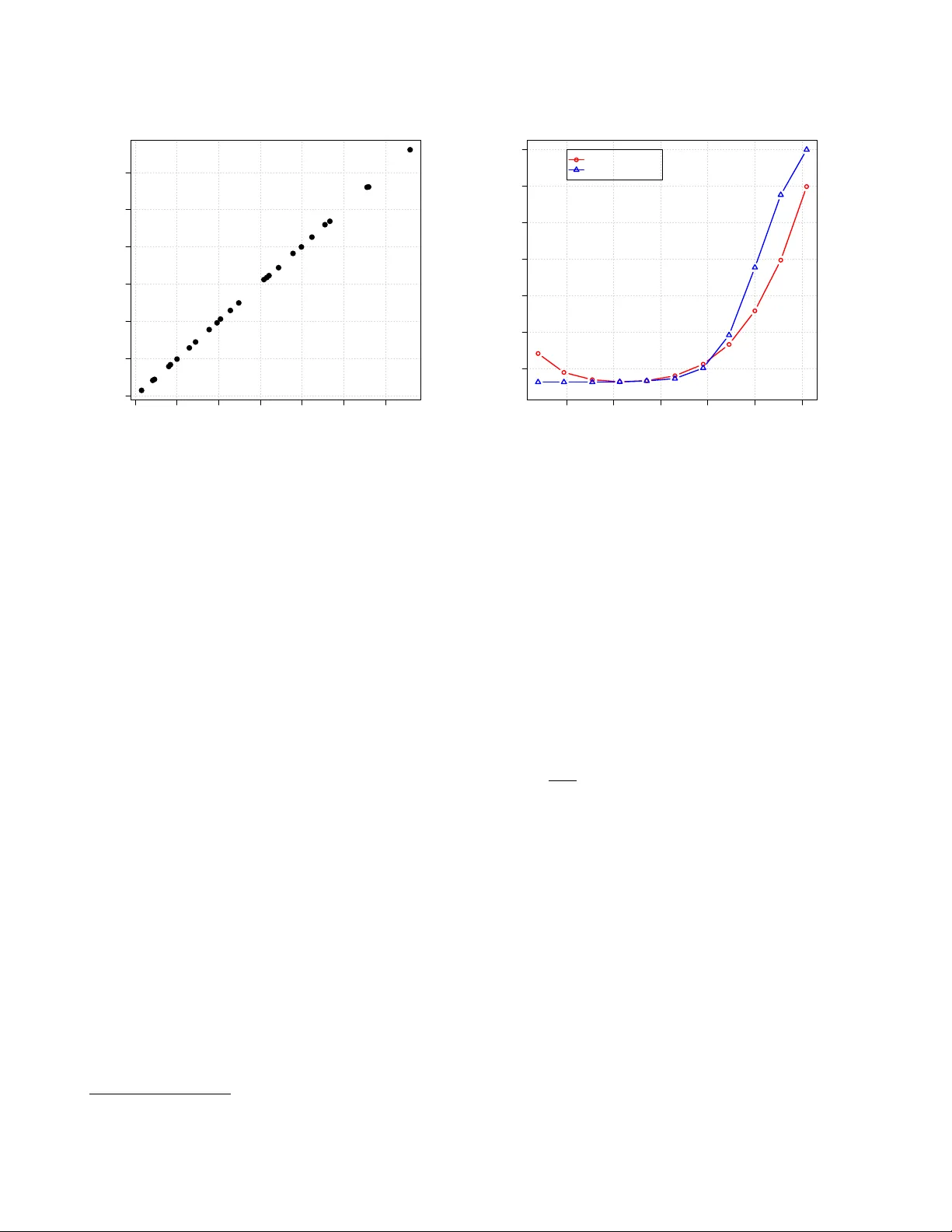
The distrib ution of calibrated likelihood-ratios in speak er r ecognition David A. van Leeuwen 1 and Niko Br ¨ ummer 2 1 Netherlands Forensic Institute, The Hague and Radboud Uni v ersity Nijme gen, The Netherlands 2 A GNITIO Research, Somerset W est, South Africa Abstract This paper studies properties of the score distributions of calibrated log-likelihood-ratios that are used in auto- matic speaker recognition. W e deriv e the essential con- dition for calibration that the log likelihood ratio of the log-likelihood-ratio is the log-likelihood-ratio. W e then in v estigate what the consequence of this condition is to the probability density functions (PDFs) of the log- likelihood-ratio score. W e show that if the PDF of the non-target distrib ution is Gaussian, then the PDF of the target distribution must be Gaussian as well. The means and v ariances of these two PDFs are interrelated, and de- termined completely by the discrimination performance of the recognizer characterized by the equal error rate. These relations allow for a new w ay of computing the offset and scaling parameters for linear calibration, and we deriv e closed-form expressions for these and show that for modern i-vector systems with PLDA scoring this leads to good calibration, comparable to traditional logis- tic regression, o ver a wide range of system performance. 1. Introduction In recent years, calibration in automatic speaker recognition has receiv ed more attention [1–11]. Intuitiv ely , calibration is related to the ability to properly set a threshold in a speaker detection system so as to minimize the expected error [12]. In speaker detection, the task is to decide whether or not two speech signals originate from the same speaker . Because all speaker recognition systems internally work with some scalar scor e that expresses speaker similarity , a score threshold can control the trade-off between the two types of errors that a sys- tem can make [13, 14]. Indeed, in the series of NIST Speaker Recognition Ev aluations (SRE) the primary ev aluation measure has been sensitive to calibration. Until SRE 2010, calibration was assessed in a single operating point, through a single de- cision cost function kno wn as C det . Also other technologies in speech technology or biometrics utilize calibration-sensiti ve ev aluation measures, such as the cost functions C avg in lan- guage recognition [15] and the Half T otal Error Rate in face recognition [16]. Since around 2004 [1,2] the concept of calibration in speaker recognition has been generalized to a range of operating points by using proper scoring rules [17] to ev aluate probabilistic statements about whether a trial is a same-speaker (target) or different-speak er (non-target) trial. A system that represents its score as a likelihood-ratio can be well-calibrated over a wide range of operating points simultaneously . This representation of the speaker recognition score has direct application in speaker detection, as the decision threshold follows directly from the cost function parameters [14], but also in evidence reporting in forensic speaker comparison cases [4, 18]. In the NIST SRE 2012, for the first time, hard decisions were no longer required, and instead the recognition score had to be submitted in the form of a likelihood-ratio. The evaluation measure ef fectiv ely sampled the decision cost function at two dif ferent parame- ters [19, 20]. Since a calibrated likelihood-ratio is still just a score, all properties of normal scores apply to likelihood-ratios as well, and we can dra w DET and R OC plots, determine EERs and inspect the score distrib utions. The axis warping of the DET plot [13] in combination with the observ ed more-or-less straight DET curves suggests that target and non-target score distribu- tions could be accurately modelled with Gaussians. These score distributions and the relation to the DET ha v e been studied pre- viously [21, 22] and are very instructi v e to the understanding of basic detection theory and the concepts of calibration [14, 23]. In this paper we are interested in properties of the distributions of calibrated log-likelihood-r atios . This may help situations were we carry out a calibration transformation on raw recog- nition scores, because it can tell us what the calibrated distribu- tions should look like. The paper is organized as follows. W e define the very na- ture of a calibrated likelihood-ratio in Section 2. In Section 3 we in v estigate the properties of log-likelihood-ratio distribu- tions when they are Gaussian, and we will then apply these in Section 4 as a new method for calibration. W e then present ex- periments and conclusions. 2. Likelihood-ratio idempotence Here we carefully define the likelihood-ratio (LR) and sho w that it has the interesting property: the LR of the LR is the LR , which forms a definition of calibration. The speaker recognition system has as input two speech segments, denoted X and Y , which it processes in two steps. W e represent the first step as s = f ( X, Y ) . T o keep things general, s may represent different kinds of output, e.g., a pair of acoustic feature vector sequences, a pair of i-vectors, or just a single, scalar recognition score. The second step is to compute the likelihood-ratio r as a function of s , as: r = P ( s | H 1 , M ) P ( s | H 2 , M ) (1) where H 1 is the (target) hypothesis that X and Y originate from the same speaker , H 2 the (non-target) hypothesis that they are from two different speakers, and M is a generati ve probabilistic model for s . In current practice, s is always the recognition score, so that M merely models scalar scores—not i-vectors, acoustic feature sequences or speech signals. But our theory below is sufficiently general to remain applicable in future to more ambitious models, when s might hav e a more complex form. W e now assume there is given the hypothesis prior , π = P ( H 1 ) , which allo ws us to express the hypothesis posterior , via Bayes’ rule as: P ( H 1 | s, M , π ) = π r π r + (1 − π ) (2) This sho ws that r is a sufficient statistic : the posterior depends on s only through r . This allo ws rewriting the posterior as: P ( h | s, M , π ) = P ( h | r , M 0 , π ) , h ∈ { H 1 , H 2 } (3) where we have introduced M 0 to denote M , augmented by as- serting (1). Although r contains all the relevant information that M can extract from s to recognize the unknown hypothe- sis, it must be stressed that r and s do not necessarily contain all the relev ant information that could ha ve been extracted from the original input X , Y by some more elaborate model. No w we use the odds form of Bayes’ rule: P ( H 1 | ρ, M , π ) P ( H 2 | ρ, M , π ) = π 1 − π P ( ρ | H 1 , M ) P ( ρ | H 2 , M ) (4) where ρ is a placeholder for r or s and M for M or M 0 . Com- bining this with (3), we find the desired relationship (the LR of the LR is the LR [24]): r = P ( s | H 1 , M ) P ( s | H 2 , M ) = P ( r | H 1 , M 0 ) P ( r | H 2 , M 0 ) . (5) If we define x to be the log-likelihood-r atio (LLR): x = log r (6) we also find 1 (the LLR of the LLR is the LLR): x = log P ( x | H 1 , M 00 ) P ( x | H 2 , M 00 ) (7) where M 00 augments M 0 by addition of (6). 2.1. Implications Rewriting (5) as: P ( r | H 1 , M 0 ) = r P ( r | H 2 , M 0 ) (8) we see that if either of the two distributions is gi ven, then the other distribution is completely determined—they cannot vary independently . Moreov er , a further restriction is placed on these distributions: since the LHS must integrate to 1 , the expected value of the non-target distribution (the integral of the RHS) must be: h r i = 1 . Similarly , for targets: h 1 r i = 1 . By applying Jensen’ s inequality [25] we also find for targets: h x i ≥ 0 and for non-targets: h x i ≤ 0 . 2.2. Good and bad calibration How does (5) function as a definition of calibration? Since it is an equality , won’t all LRs calculated via (1) by some model M , just automatically satisfy (5)? Y es they will, but only if M and M 0 are related as explained above. If we want to independently judge the goodness of the calibration of r , we do not condition the distributions for r on the recognizer’ s model M . Instead, we could empirically observe the target and non-target values 1 T o see this, note the log transformation is monotonic and the Jaco- bian of the transformation cancels in the ratio. of r as calculated by the recognizer over an independent, super- vised database of speaker detection trials. Letting O denote the empirical observ ation, we could then say the model M is well calibrated if: r = P ( s | H 1 , M ) P ( s | H 2 , M ) ≈ P ( r | H 1 , O ) P ( r | H 2 , O ) (9) Bad calibration is when the LRs giv en respecti vely by the rec- ognizer’ s M and empirical observation O , do not agree in this way . This can and does happen, since O is independent of any dev elopment data that was used to determine the form and pa- rameters of M . It should be noted that (9) does not giv e a practical recipe to judge degree of goodness of calibration—it specifies neither how to assign P ( r | h, O ) , nor how to numerically e v aluate the agreement between LHS and RHS. For practical solutions for calibration-sensitiv e objecti ve functions, see for e xample [26]. 3. Gaussian distributed log-likelihood-ratios Inspired by the fact that DET curv es in speaker recognition tend to be straight [21], we explore a Gaussian solution to the LLR distrib ution constraint (7). Since tar get and non-target LLR distrib utions are so tightly coupled, it turns out that if the one is assumed to be Gaussian, then the other must also be. W e shall use the shorthand: e ( x ) = P ( x | H 1 , M 00 ) and d ( x ) = P ( x | H 2 , M 00 ) . Arbitrarily assuming a Gaussian dis- tribution for non-tar gets ( dif ferent -speaker trials): d ( x ) = N ( x | µ d , σ d ) = 1 √ 2 π σ d e − ( x − µ d ) 2 / 2 σ 2 d . (10) W e deriv e the functional form for targets 2 , e ( x ) , when (7) ap- plies: e ( x ) = e x d ( x ) = 1 √ 2 π σ d e x − ( x − µ d ) 2 / 2 σ 2 d . (11) W e collect the terms in x in the exponent, which itself can be written like − x 2 − 2 µ d x + µ 2 d 2 σ 2 d + 2 σ 2 d x 2 σ 2 d (12) = − x 2 − 2( µ d + σ 2 d ) x + µ 2 d 2 σ 2 d (13) = −  x − ( µ d + σ 2 d )  2 2 σ 2 d + 2 µ d σ 2 d + σ 4 d 2 σ 2 d (14) The first term is in the familiar form of a Gaussian exponent, the second will result in a constant f actor . Gathering terms, and writing µ e = µ d + σ 2 d , (15) the expression for the same-speaker comparison log-likelihood- ratio scores becomes e ( x ) = 1 √ 2 π σ d e σ 2 d / 2+ µ d e − ( x − µ 2 e ) / 2 σ 2 d (16) = e σ 2 d / 2+ µ d N ( x | µ e , σ d ) . (17) W e see that e ( x ) is of Gaussian shape, with σ e = σ d ≡ σ. (18) 2 trials where the speakers are equal Since e ( x ) must be a proper PDF , its integral over x must be unity , from which follows that e σ 2 / 2+ µ d Z ∞ −∞ N ( x | µ e , σ ) dx = 1 (19) − 2 µ d = σ 2 . (20) Finally , with (15) we find µ e = µ d + σ 2 = − µ d ≡ µ, (21) This sho ws that d ( x ) and e ( x ) are equal variance Gaussians with means symmetric around zero at ± µ , and where the v ari- ance and mean are related (20) σ 2 = 2 µ. (22) 3.1. Equal Error Rate and d 0 Using the symmetry of the solution, it is clear that the threshold for the equal error rate is at x = 0 . Using the e xpression for the miss probability , the equal error rate E = is E = = Z 0 −∞ N ( x | µ, σ ) (23) = Z − µ/σ −∞ N ( x | 0 , 1) ≡ Φ( − µ/σ ) , (24) where Φ( x ) is the cumulativ e normal distribution. It is sometimes useful to recognize the parameter d 0 from detection theory , which is the difference in means expressed in terms of the standard deviation, here d 0 = 2 µ/σ . W ith (24) the relation becomes E = = Φ( − 1 2 d 0 ) . (25) d 0 = σ = − 2Φ − 1 ( E = ) , (26) introducing Φ − 1 ( y ) , the inv erse of the cumulative normal dis- tribution. The importance of the relations abov e is that µ and σ are determined by the discrimination performance measured by E = , using (22) and (26) µ = σ 2 2 = 2[Φ − 1 ( E = )] 2 . (27) 4. A new calibration method In practice, automatic speaker recognition systems do not de- liv er scores that can directly be interpreted as a log-likelihood- ratio, even though they are computed as such, for instance in the good old UBM-GMM scoring [27] or the latest i-vector PLD A scoring [28]. A practical solution to this is to conv ert raw scores s ( X , Y ) to calibrated log-likelihood-ratios by some transformation function x ( s ) , usually constrained to be mono- tonic increasing. There are many ways of doing this. The Fo- Cal [29] and BOSARIS [30] toolkits use logistic regression to discriminativ ely train linear calibration transformations. Other possibilities include isotonic regression (P A V [30]) and line-up calibration [9] that uses the rank in a line-up of foil speakers. In FoCal or BOSARIS, the score-to-LLR function is af fine: x ( s ) = as + b (28) and the parameters a and b are found by optimizing cross- entropy , a calibration-sensitive objectiv e function defined on a supervised set of speaker recognition trials. Here we contrast the popular discriminativ e logistic re- gression solution to a new generative, constrained maximum- likelihood (ML) solution. Our constraints follow from assum- ing (i) Gaussian LLR distributions, and (ii) an affine score-to- LLR transform (28). This implies that (i) the LLR distributions are constrained as deri ved in Section 3, and (ii) the score dis- tributions are also Gaussians, with equal v ariances. W ith no LLR distribution constraints, we would have had 6 free param- eters: 2 means, 2 variances and 2 calibration parameters. But we have imposed 3 constraints, equal variances (18), symmetric means (21) and (22). W e find the remaining 3 free parameters by maximizing the following weighted lik elihood: α N e X i ∈E log N ( s i | m e , v ) + 1 − α N d X i ∈D log N ( s i | m d , v ) where E and D index N e target, and N d non-target scores, weighted by α and 1 − α , respectively . The score distribution parameters that need to be optimized are the means m e , m d and common variance v . Setting deriv ati ves to 0 , we find the maxi- mum likelihood at the sample means: m e = 1 N e X i ∈E s i , m d = 1 N d X i ∈D s i (29) and at a weighted combination of sample variances: v = α N e X i ∈E ( s i − m e ) 2 + 1 − α N d X i ∈D ( s i − m d ) 2 (30) By (28), the LLR distribution parameters become σ 2 = a 2 v , µ e = am e + b and µ d = am d + b . Finally , applying the constraints σ 2 = µ e − µ d and µ e = − µ d , we can solve for the calibration parameters: a = m e − m d v , b = − a m e + m d 2 (31) W e call this recipe constr ained, maximum-likelihood, Gaussian (CMLG) calibration. An adv antage of CMLG is that it has a closed form, in contrast to the iterativ e optimization required by logistic regression. 4.1. Experiment In order to test CMLG we apply it to a number of recognition trials sets. W e use a set of trials crafted for duration-dependence experiments [8] from the NIST SRE 2008 and 2010 trial sets, the telephone-telephone “extended” trial lists. W e constructed short duration segments of 5, 10, 20, and 40 seconds from both train and test segments by simply selecting the first frames af- ter speech activity detection. All durations, including the full con versation side, were tested in all combinations, leading to 25 different trial lists. The NIST SRE10 ‘det-5’ performance ov er these lists ranges from E = = 2 . 9 – 26 %. The recognition system is a standard i-vector based system with PLD A scoring described elsewhere [20]. W e contrast CMLG (with α = 1 2 ) to the traditional logistic regression method. The calibrations are trained on NIST SRE 2008 data (427 375 trials) and applied to SRE 2010 trials for ev aluation (10 007 900 trials), all gender mixed. W e e valuate the 25 different trial list combinations using C llr , a cost function that is sensitive to calibration over the whole DET curve [2]. W e used R’ s glm routine for logistic regression. The results are shown in Fig. 1, where we have plotted the C llr obtained using CMLG calibration versus C llr obtained us- ing logistic regression. The values are highly correlated. For 0.1 0.2 0.3 0.4 0.5 0.6 0.7 0.1 0.2 0.3 0.4 0.5 0.6 0.7 Correlation in Cllr for different calibration methods constrained maximum likelihood Gaussian (CMLG) logistic regression Figure 1: C llr values of the 25 trial lists for the CMLG method (horizontal) versus logistic re gression (vertical). CMLG, the a verage C llr ov er all 25 conditions is 0.375, for lo- gistic regression it is 0.376. These can be called good, as the mean C min llr is 0.370. W e ha ve also used the NIST SRE12 scores from the ABC- team to study the effect of α in (30) to another calibration sen- sitiv e measure C primary , cf. Fig. 2, for details we refer to [26]. The figure shows that with CMLG good calibration results can be obtained for a different system with dif ferent data and a dif- ferent performance measure, if the correct α is chosen. 5. Discussion and Conclusions W e have shown in this paper , that if the different-speaker cal- ibrated log-likelihood-ratio scores from a speaker recognition system follow a Gaussian distribution, then the distribution of the same-speaker scores must also be Gaussian after calibra- tion, with the same variance but opposite mean. Because mono- tonically increasing score-to-likelihood-ratio functions do not change the DET plot, such equal-variance distributions in the calibrated score domain imply 45 ◦ DET -plots in the raw score domain as well—which is neither observed with real data 3 nor desired for applications operating in the low false alarm re gion. The logical conclusion then is that real scores, if they are well- calibrated, will not be Gaussian. Howev er , we see that our PLD A system can be calibrated quite well under the Gaussian assumptions, and indeed we have noticed that i-vector PLDA systems tend to hav e score distributions that appear more Gaus- sian than earlier technologies, such as i-vector LD A cosine dis- tance scoring, support vector machines or the UBM-GMM like- lihood ratio scoring. The Gaussian solution to the LLR equation (7) is one where both distributions are shaped by the same mathematical func- tion. In signal detection theory , where the distribution repre- sents noise, this seems almost mandatory , b ut in speaker recog- nition this is not an obvious assumption. W e ha ve experimented with other distributions, e.g., in the likelihood-ratio domain (5) 3 W e hav e measured the slope of the DET in the conv entional error region 0.1–50 % for the data in the experiment. The mean slope over the 25 conditions is − 0 . 99 with a standard deviation of 0 . 06 , so in f act this data appears to honour the equal variance condition quite well. -8 -6 -4 -2 0 2 0.30 0.35 0.40 0.45 0.50 0.55 0.60 Comparison of calibration methods log ( α ) − log ( 1 − α ) C p r i m a r y logistic regression CMLG Figure 2: C primary for logistic regression and CMLG calibra- tion methods for ABC’ s SRE12 submission, as a function of prior α used in the objectiv e / ML optimization. a pair of Gamma distributions is a solution to the calibration condition, and these are asymmetric in the log-likelihood-ratio domain. Howev er , such distributions seem to be not at all rep- resentativ e of real score distributions. Also, an arbitrary linear combination of Gaussians with dif ferent means and correspond- ing variances is a solution to (7) which allo ws some freedom in fitting a shape of score distribution. In principle, there is no need for real score distrib utions to follow any mathematical de- scription, but we have observed that many researchers like to use some form of idealized shape of the score distributions to understand the data [4, 21]. When calibration methods are de- signed, condition (7) should therefore be taken into account. The relations derived in Section 3 open up more possibili- ties for relations between the v arious e valuation measures. For instance, we can compute C llr by numerical integration as 1 log 2 Z ∞ −∞ N ( x | µ, σ ) log (1 + e − x ) dx (32) and this relates C llr to E = via (26) and (27) for Gaussian score distributions. E.g., for our set of 25 trial lists this expression differs from C min llr only 0.006 in root mean squared dif ference, or about 2 %. Instead of for calibration, the relations can also be used for fusion of systems. For pre-calibrated systems this leads to solutions that transparently depend on the correlation between the scores. The fact that we can obtain the linear calibration parame- ters under the Gaussian assumption is an interesting side-effect of this study . The calibration parameters can be expressed in closed-form, and do not explicitly consider cross entropy or C llr as an optimization objectiv e. For score distrib utions that do not resemble a Gaussian, this calibration method is likely to fail— we therefore do not recommend CMLG calibration as a general technique. Still, we are quite pleased that the experiments sup- port the mostly theoretical results of this paper . 6. Acknowledgments The research leading to these results has received funding from the European Community’ s Se venth Frame work Programme (FP7/2007–2013) under grant agreement no. 238803. 7. References [1] N. Br ¨ ummer , “ Application-independent ev aluation of speaker detection, ” in Pr oc. Odysse y 2004 Speaker and Language reco gnition workshop . ISCA, June 2004, pp. 33–40. [2] N. Br ¨ ummer and J. du Preez, “ Application-independent ev aluation of speaker detection, ” Computer Speech and Language , v ol. 20, pp. 230–275, 2006. [3] N. Br ¨ ummer and D. A. van Leeuwen, “On calibration of language recognition scores, ” in Pr oc. Odyssey 2006 Speaker and Language r ecognition workshop , San Juan, June 2006. [4] D. Ramos-Castro, J. Gonz ´ alez-Rodr ´ ıguez, and J. Ortega- Garcia, “Likelihood ratio calibration in a transparent and testable forensic speaker recognition framework, ” in Pr oc. Odysse y 2006 Speaker and Language Recognition W ork- shop , 2006. [5] D. Ramos, “Forensic ev aluation of the evidence using au- tomatic speaker recognition systems, ” Ph.D. dissertation, Univ ersidad Autonoma de Madrid, November 2007. [6] N. Br ¨ ummer , L. Burget, J. ˇ Cernock ´ y, O. Glembek, F . Grezl, M. Karafi ´ at, P . Mat ˇ ejka, D. A. van Leeuwen, P . Schwarz, and A. Strassheim, “Fusion of heterogeneous speaker recognition systems in the STBU submission for the NIST speaker recognition ev aluation 2006, ” IEEE T ransactions on Speech, Audio and Language Processing , vol. 15, no. 7, pp. 2072–2084, 2007. [7] Z. Jancik, O. Plchot, N. Brummer, L. Burget, O. Glem- bek, V . Hubeika, M. Karafi ´ at, P . Matejka, T . Mikolov , A. Strasheim et al. , “Data selection and calibration issues in automatic language recognition–inv estigation with BUT -AGNITIO NIST LRE 2009 system, ” in Pr oc. Speaker and Languag e Odysse y , 2010. [8] M. I. Mandasari, M. McLaren, and D. A. van Leeuwen, “Evaluation of i-v ector speaker recognition systems for forensic application, ” in Pr oc. Inster speech . Firenze: ISCA, August 2011. [9] D. A. van Leeuwen and N. Br ¨ ummer , “ A speaker line-up for the likelihood ratio, ” in Pr oc. Interspeech . Firenze: ISCA, August 2011. [10] M. I. Mandasari, M. McLaren, and D. A. van Leeuwen, “The ef fect of noise on modern automatic speaker recog- nition systems, ” in Pr oc. ICASSP . K yoto: IEEE, March 2012. [11] G. R. Doddington, “The role of score calibration in speaker recognition, ” in Pr oc. Interspeech , 2012. [12] G. R. Doddington, M. A. Przybocki, A. F . Martin, and D. A. Reynolds, “The NIST speaker recognition ev aluation—Overvie w , methodology , systems, results, perspectiv e, ” Speech Communication , v ol. 31, pp. 225– 254, 2000. [13] A. Martin, G. Doddington, T . Kamm, M. Ordowski, and M. Przybocki, “The DET curve in assessment of detection task performance, ” in Pr oc. Eur ospeech 1997 , Rhodes, Greece, 1997, pp. 1895–1898. [14] D. A. van Leeuwen and N. Br ¨ ummer , “ An introduction to application-independent evaluation of speaker recognition systems, ” in Speaker Classification , ser . Lecture Notes in Computer Science / Artificial Intelligence, C. M ¨ uller , Ed. Springer , 2007, vol. 4343. [15] A. F . Martin and A. N. Le, “NIST 2007 language recogni- tion e valuation, ” in Proc. Speaker and Language Odysse y . Stellenbosch, South Afrika: IEEE, 2008. [16] R. W allace, M. McLaren, C. McCool, and S. Mar- cel, “Cross-pollination of normalization techniques from speaker to face authentication using gaussian mixture models, ” Information F orensics and Security , IEEE T rans- actions on , vol. 7, no. 2, pp. 553–562, 2012. [17] M. DeGroot and S. Fienberg, “The comparison and ev al- uation of forecasters, ” The Statistician , pp. 12–22, 1983. [18] J. Gonzalez-Rodriguez, P . Rose, D. Ramos, D. T . T oledano, and J. Ortega-Garcia, “Emulating DN A: Rigor- ous quantification of evidential weight in transparent and testable forensic speaker recognition, ” IEEE T ransactions on Audio, Speech and Language Pr ocessing , vol. 15, no. 7, pp. 2104–2115, September 2007. [19] C. S. Greenberg, “The NIST year 2012 speaker recognition ev aluation plan, ” 2012. [On- line]. A vailable: http://www .nist.gov/itl/iad/mig/upload/ NIST SRE12 ev alplan- v17- r1.pdf [20] D. A. van Leeuwen and R. Saeidi, “Kno wing the non- target speakers: the effect of the i-vector population for PLD A training in speaker recognition, ” in Proc ICASSP . V ancouver: IEEE, 2013. [21] R. Auck enthaler, M. Care y , and H. Lloyd-Thomas, “Score normalization for text-independent speaker verification systems, ” Digital Signal Pr ocessing , vol. 10, pp. 42–54, 2000. [22] J. Navr ´ atil and G. N. Ramsawamy , “The awe and mistery of t-norm, ” in Proc. Eur ospeech , 2003, pp. 2009–2012. [23] N. Br ¨ ummer , “Measuring, refining and calibrating speaker and language information extracted from speech, ” Ph.D. dissertation, Stellenbosch Univ ersity , 2010. [24] K. Slooten and R. Meester, “Forensic identification: Database likelihood ratios and familial DNA searching, ” arXiv:1201.4261 [stat.AP] , 2012. [25] J. L. W . V . Jensen, “Sur les fonctions con vexes et les in ´ egalit ´ es entre les valeurs moyennes, ” Acta Mathematica , vol. 30, no. 1, pp. 175–193, 1906. [26] N. Br ¨ ummer and G. Doddington, “Likelihood-ratio cal- ibration using prior-weighted proper scoring rules, ” in Pr oc. Interspeech . ISCA, 2013. [27] D. A. Reynolds, T . F . Quatieri, and R. B. Dunn, “Speaker verification using adapted gaussian mixture models, ” Dig- ital Signal Pr ocessing , vol. 10, pp. 19–41, 2000. [28] S. J. D. Prince and J. H. Elder , “Probabilistic linear dis- criminant analysis for inferences about identity , ” in IEEE International Conference on Computer V ision (ICCV) . IEEE, 2007, pp. 1–8. [29] N. Br ¨ ummer , F oCal-II: T oolkit for calibration of multi- class reco gnition scores , August 2006, software av ailable at http://www .dsp.sun.ac.za/ ∼ nbrummer/focal/index.htm. [30] E. de V illiers and N. Br ¨ ummer , The Bosaris T oolkit , BOSARIS, 2010, software a vailable at https://sites. google.com/site/bosaristoolkit/.