From Softmax to Sparsemax: A Sparse Model of Attention and Multi-Label Classification

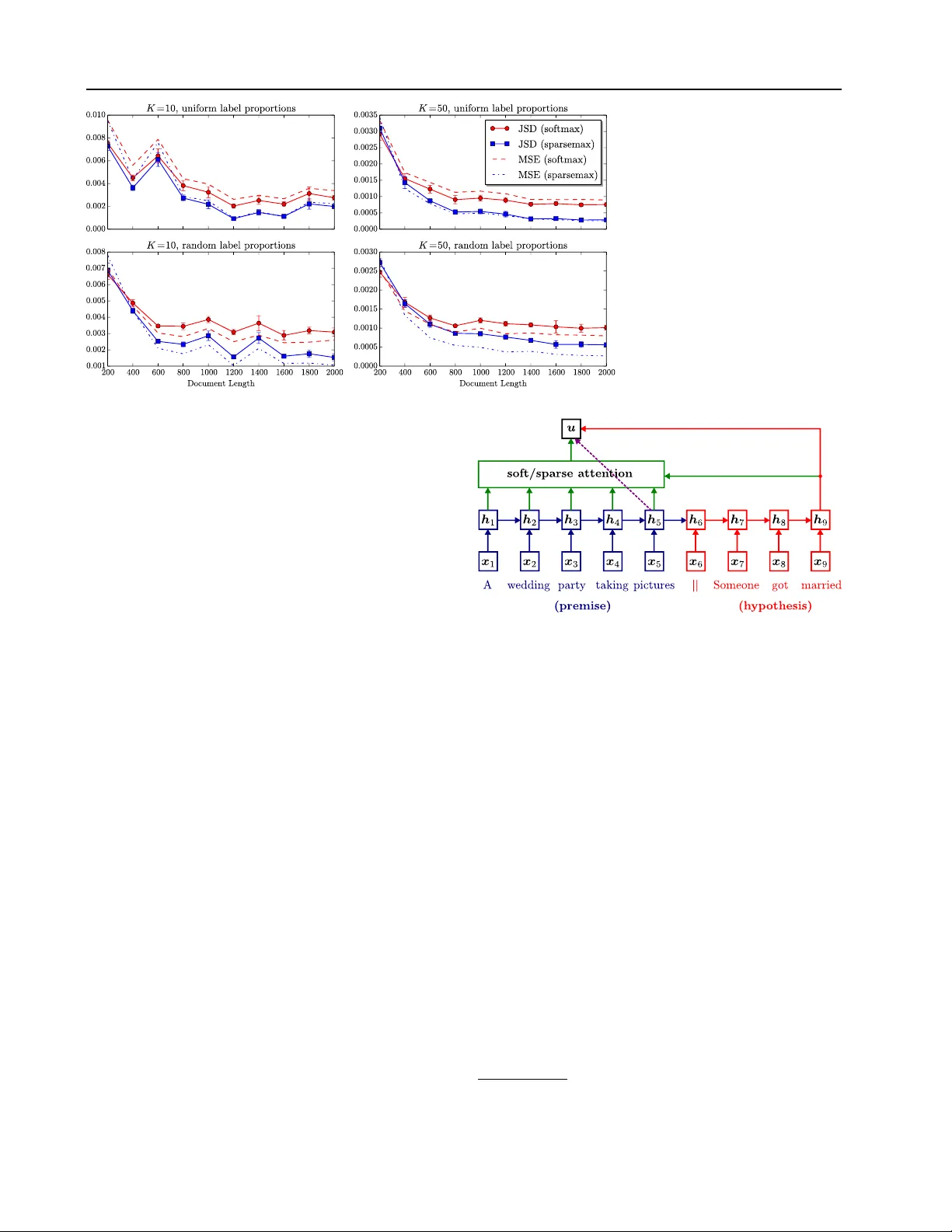
Fr om Softmax to Sparsemax: A Sparse Model of Attention and Multi-Label Classification Andr ´ e F . T . Martins † ] A N D R E . M A RT I N S @ U N BA B E L . C O M Ram ´ on F . Astudillo † R A M O N @ U N BA B E L . C O M † Unbabel Lda, Rua V isconde de Santar ´ em, 67-B, 1000-286 Lisboa, Portugal ] Instituto de T elecomunicac ¸ ˜ oes (IT), Instituto Superior T ´ ecnico, A v . Rovisco P ais, 1, 1049-001 Lisboa, Portugal  Instituto de Engenharia de Sistemas e Computadores (INESC-ID), Rua Alves Redol, 9, 1000-029 Lisboa, Portugal Abstract W e propose sparsemax, a new activ ation func- tion similar to the traditional softmax, b ut able to output sparse probabilities. After deriving its properties, we show how its Jacobian can be efficiently computed, enabling its use in a net- work trained with backpropagation. Then, we propose a new smooth and conv ex loss function which is the sparsemax analogue of the logis- tic loss. W e re veal an unexpected connection between this new loss and the Huber classifi- cation loss. W e obtain promising empirical re- sults in multi-label classification problems and in attention-based neural networks for natural lan- guage inference. For the latter , we achie ve a sim- ilar performance as the traditional softmax, but with a selectiv e, more compact, attention focus. 1. Introduction The softmax transformation is a key component of se veral statistical learning models, encompassing multinomial lo- gistic regression (McCullagh & Nelder, 1989), action se- lection in reinforcement learning (Sutton & Barto, 1998), and neural networks for multi-class classification (Bridle, 1990; Goodfellow et al., 2016). Recently , it has also been used to design attention mechanisms in neural networks, with important achiev ements in machine translation (Bah- danau et al., 2015), image caption generation (Xu et al., 2015), speech recognition (Chorowski et al., 2015), mem- ory networks (Sukhbaatar et al., 2015), and various tasks in natural language understanding (Hermann et al., 2015; Rockt ¨ aschel et al., 2015; Rush et al., 2015) and computa- tion learning (Gra ves et al., 2014; Grefenstette et al., 2015). There are a number of reasons why the softmax transfor- mation is so appealing. It is simple to ev aluate and dif- ferentiate, and it can be turned into the (con vex) negativ e log-likelihood loss function by taking the logarithm of its output. Alternati ves proposed in the literature, such as the Bradley-T erry model (Bradley & T erry, 1952; Zadrozn y, 2001; Menke & Martinez, 2008), the multinomial probit (Albert & Chib, 1993), the spherical softmax (Ollivier, 2013; V incent, 2015; de Br ´ ebisson & V incent, 2015), or softmax approximations (Bouchard, 2007), while theoret- ically or computationally advantageous for certain scenar - ios, lack some of the con venient properties of softmax. In this paper , we propose the sparsemax transformation . Sparsemax has the distinctive feature that it can return sparse posterior distrib utions, that is, it may assign exactly zero probability to some of its output variables. This prop- erty makes it appealing to be used as a filter for large out- put spaces, to predict multiple labels, or as a component to identify which of a group of variables are potentially rele- vant for a decision, making the model more interpretable. Crucially , this is done while preserving most of the attrac- tiv e properties of softmax: we show that sparsemax is also simple to ev aluate, it is ev en cheaper to differentiate, and that it can be turned into a con vex loss function. T o sum up, our contrib utions are as follows: • W e formalize the new sparsemax transformation, de- riv e its properties, and show how it can be ef ficiently computed ( § 2.1 – 2.3). W e sho w that in the binary case sparsemax reduces to a hard sigmoid ( § 2.4). • W e deriv e the Jacobian of sparsemax, comparing it to the softmax case, and show that it can lead to faster gradient backpropagation ( § 2.5). • W e propose the sparsemax loss , a new loss function that is the sparsemax analogue of logistic regression ( § 3). W e show that it is conv ex, ev erywhere dif feren- tiable, and can be regarded as a multi-class general- ization of the Huber classification loss, an important tool in robust statistics (Huber, 1964; Zhang, 2004). From Softmax to Sparsemax: A Sparse Model of Attention and Multi-Label Classification • W e apply the sparsemax loss to train multi-label linear classifiers (which predict a set of labels instead of a single label) on benchmark datasets ( § 4.1 – 4.2). • Finally , we devise a neural selectiv e attention mecha- nism using the sparsemax transformation, ev aluating its performance on a natural language inference prob- lem, with encouraging results ( § 4.3). 2. The Sparsemax T ransformation 2.1. Definition Let ∆ K − 1 := { p ∈ R K | 1 > p = 1 , p ≥ 0 } be the ( K − 1) -dimensional simplex. W e are interested in functions that map vectors in R K to probability distrib utions in ∆ K − 1 . Such functions are useful for con verting a vector of real weights ( e.g. , label scores) to a probability distrib ution ( e.g . posterior probabilities of labels). The classical example is the softmax function , defined componentwise as: softmax i ( z ) = exp( z i ) P j exp( z j ) . (1) A limitation of the softmax transformation is that the re- sulting probability distribution always has full support, i.e . , softmax i ( z ) 6 = 0 for every z and i . This is a disadvan- tage in applications where a sparse probability distribution is desired, in which case it is common to define a threshold below which small probability v alues are truncated to zero. In this paper , we propose as an alternative the following transformation, which we call sparsemax : sparsemax( z ) := argmin p ∈ ∆ K − 1 k p − z k 2 . (2) In words, sparsemax returns the Euclidean projection of the input vector z onto the probability simplex. This projection is likely to hit the boundary of the simplex, in which case sparsemax( z ) becomes sparse. W e will see that sparsemax retains most of the important properties of softmax, ha ving in addition the ability of producing sparse distributions. 2.2. Closed-Form Solution Projecting onto the simplex is a well studied problem, for which linear-time algorithms are available (Michelot, 1986; Pardalos & Ko voor, 1990; Duchi et al., 2008). W e start by recalling the well-known result that such projections corre- spond to a soft-thresholding operation. Below , we use the notation [ K ] := { 1 , . . . , K } and [ t ] + := max { 0 , t } . Proposition 1 The solution of Eq. 2 is of the form: sparsemax i ( z ) = [ z i − τ ( z )] + , (3) wher e τ : R K → R is the (unique) function that satis- fies P j [ z j − τ ( z )] + = 1 for e very z . Furthermor e, τ Algorithm 1 Sparsemax Evaluation Input: z Sort z as z (1) ≥ . . . ≥ z ( K ) Find k ( z ) := max n k ∈ [ K ] | 1 + k z ( k ) > P j ≤ k z ( j ) o Define τ ( z ) = ( P j ≤ k ( z ) z ( j ) ) − 1 k ( z ) Output: p s.t. p i = [ z i − τ ( z )] + . can be expr essed as follows. Let z (1) ≥ z (2) ≥ . . . ≥ z ( K ) be the sorted coordinates of z , and define k ( z ) := max n k ∈ [ K ] | 1 + k z ( k ) > P j ≤ k z ( j ) o . Then, τ ( z ) =  P j ≤ k ( z ) z ( j )  − 1 k ( z ) =  P j ∈ S ( z ) z j  − 1 | S ( z ) | , (4) wher e S ( z ) := { j ∈ [ K ] | sparsemax j ( z ) > 0 } is the support of sparsemax( z ) . Pr oof: See App. A.1 in the supplemental material. In essence, Prop. 1 states that all we need for ev aluating the sparsemax transformation is to compute the threshold τ ( z ) ; all coordinates above this threshold (the ones in the set S ( z ) ) will be shifted by this amount, and the others will be truncated to zero. W e call τ in Eq. 4 the threshold func- tion . This piecewise linear function will play an important role in the sequel. Alg. 1 illustrates a na ¨ ıve O ( K log K ) algorithm that uses Prop. 1 for ev aluating the sparsemax. 1 2.3. Basic Properties W e now highlight some properties that are common to soft- max and sparsemax. Let z (1) := max k z k , and denote by A ( z ) := { k ∈ [ K ] | z k = z (1) } the set of maximal compo- nents of z . W e define the indicator vector 1 A ( z ) , whose k th component is 1 if k ∈ A ( z ) , and 0 otherwise. W e further denote by γ ( z ) := z (1) − max k / ∈ A ( z ) z k the gap between the maximal components of z and the second largest. W e let 0 and 1 be vectors of zeros and ones, respectiv ely . Proposition 2 The following pr operties hold for ρ ∈ { softmax , sparsemax } . 1. ρ ( 0 ) = 1 /K and lim  → 0 + ρ (  − 1 z ) = 1 A ( z ) / | A ( z ) | (uniform distribution, and distribution peaked on the maximal components of z , respectively). F or sparse- max, the last equality holds for any  ≤ γ ( z ) · | A ( z ) | . 2. ρ ( z ) = ρ ( z + c 1 ) , for any c ∈ R ( i.e. , ρ is in variant to adding a constant to each coor dinate). 1 More elaborate O ( K ) algorithms exist based on linear-time selection (Blum et al., 1973; Pardalos & K ovoor, 1990). From Softmax to Sparsemax: A Sparse Model of Attention and Multi-Label Classification − 3 − 2 − 1 0 1 2 3 t 0 . 0 0 . 2 0 . 4 0 . 6 0 . 8 1 . 0 s o f t ma x 1 ( [t , 0 ]) s pa r s e ma x 1 ( [t , 0 ]) t 1 − 3 − 2 − 1 0 1 2 3 t 2 − 3 − 2 − 1 0 1 2 3 s pa r s e ma x 1 ( [t 1 , t 2 , 0 ]) 0 . 0 0 . 2 0 . 4 0 . 6 0 . 8 1 . 0 t 1 − 3 − 2 − 1 0 1 2 3 t 2 − 3 − 2 − 1 0 1 2 3 s o f t ma x 1 ( [t 1 , t 2 , 0 ]) 0 . 0 0 . 2 0 . 4 0 . 6 0 . 8 1 . 0 Figure 1. Comparison of softmax and sparsemax in 2D (left) and 3D (two righmost plots). 3. ρ ( P z ) = P ρ ( z ) for any permutation matrix P ( i.e. , ρ commutes with permutations). 4. If z i ≤ z j , then 0 ≤ ρ j ( z ) − ρ i ( z ) ≤ η ( z j − z i ) , wher e η = 1 2 for softmax, and η = 1 for sparsemax. Pr oof: See App. A.2 in the supplemental material. Interpreting  as a “temperature parameter, ” the first part of Prop. 2 shows that the sparsemax has the same “zero- temperature limit” behaviour as the softmax, but without the need of making the temperature arbitrarily small. Prop. 2 is reassuring, since it sho ws that the sparsemax transformation, despite being defined very dif ferently from the softmax, has a similar behaviour and preserves the same in variances. Note that some of these properties are not sat- isfied by other proposed replacements of the softmax: for example, the spherical softmax (Ollivier, 2013), defined as ρ i ( z ) := z 2 i / P j z 2 j , does not satisfy properties 2 and 4. 2.4. T wo and Thr ee-Dimensional Cases For the two-class case, it is well known that the softmax activ ation becomes the logistic (sigmoid) function. More precisely , if z = ( t, 0) , then softmax 1 ( z ) = σ ( t ) := (1 + exp( − t )) − 1 . W e next show that the analogous in sparsemax is the “hard” version of the sigmoid. In fact, using Prop. 1, Eq. 4, we hav e that, for z = ( t, 0) , τ ( z ) =    t − 1 , if t > 1 ( t − 1) / 2 , if − 1 ≤ t ≤ 1 − 1 , if t < − 1 , (5) and therefore sparsemax 1 ( z ) =    1 , if t > 1 ( t + 1) / 2 , if − 1 ≤ t ≤ 1 0 , if t < − 1 . (6) Fig. 1 provides an illustration for the two and three- dimensional cases. For the latter , we parameterize z = ( t 1 , t 2 , 0) and plot softmax 1 ( z ) and sparsemax 1 ( z ) as a function of t 1 and t 2 . W e can see that sparsemax is piece- wise linear , but asymptotically similar to the softmax. 2.5. Jacobian of Sparsemax The Jacobian matrix of a transformation ρ , J ρ ( z ) := [ ∂ ρ i ( z ) /∂ z j ] i,j , is of key importance to train models with gradient-based optimization. W e next deriv e the Jacobian of the sparsemax activ ation, but before doing so, let us re- call how the Jacobian of the softmax looks lik e. W e hav e ∂ softmax i ( z ) ∂ z j = δ ij e z i P k e z k − e z i e z j ( P k e z k ) 2 = softmax i ( z )( δ ij − softmax j ( z )) , (7) where δ ij is the Kronecker delta, which ev aluates to 1 if i = j and 0 otherwise. Letting p = softmax( z ) , the full Jacobian can be written in matrix notation as J softmax ( z ) = Diag ( p ) − pp > , (8) where Diag ( p ) is a matrix with p in the main diagonal. Let us now turn to the sparsemax case. The first thing to note is that sparsemax is differentiable e verywhere except at splitting points z where the support set S ( z ) changes, i.e. , where S ( z ) 6 = S ( z +  d ) for some d and infinitesimal  . 2 From Eq. 3, we hav e that: ∂ sparsemax i ( z ) ∂ z j = ( δ ij − ∂ τ ( z ) ∂ z j , if z i > τ ( z ) , 0 , if z i ≤ τ ( z ) . (9) It remains to compute the gradient of the threshold function τ . From Eq. 4, we hav e: ∂ τ ( z ) ∂ z j =  1 | S ( z ) | if j ∈ S ( z ) , 0 , if j / ∈ S ( z ) . (10) Note that j ∈ S ( z ) ⇔ z j > τ ( z ) . Therefore we obtain: ∂ sparsemax i ( z ) ∂ z j =  δ ij − 1 | S ( z ) | , if i, j ∈ S ( z ) , 0 , otherwise. (11) 2 For those points, we can take an arbitrary matrix in the set of generalized Clarke’ s Jacobians (Clarke, 1983), the con ve x hull of all points of the form lim t →∞ J sparsemax ( z t ) , where z t → z . From Softmax to Sparsemax: A Sparse Model of Attention and Multi-Label Classification Let s be an indicator vector whose i th entry is 1 if i ∈ S ( z ) , and 0 otherwise. W e can write the Jacobian matrix as J sparsemax ( z ) = Diag ( s ) − ss > / | S ( z ) | . (12) It is instructi ve to compare Eqs. 8 and 12. W e may re- gard the Jacobian of sparsemax as the Laplacian of a graph whose elements of S ( z ) are fully connected. T o compute it, we only need S ( z ) , which can be obtained in O ( K ) time with the same algorithm that ev aluates the sparsemax. Often, e.g . , in the gradient backpropagation algorithm, it is not necessary to compute the full Jacobian matrix, but only the product between the Jacobian and a giv en vector v . In the softmax case, from Eq. 8, we hav e: J softmax ( z ) · v = p  ( v − ¯ v 1 ) , with ¯ v := P j p j v j , (13) where  denotes the Hadamard product; this requires a linear-time computation. For the sparsemax case, we ha ve: J sparsemax ( z ) · v = s  ( v − ˆ v 1 ) , with ˆ v := P j ∈ S ( z ) v j | S ( z ) | . (14) Interestingly , if sparsemax( z ) has already been ev aluated ( i.e. , in the forward step), then so has S ( z ) , hence the nonzeros of J sparsemax ( z ) · v can be computed in only O ( | S ( z ) | ) time, which can be sublinear . This can be an im- portant adv antage of sparsemax over softmax if K is large. 3. A Loss Function f or Sparsemax Now that we hav e defined the sparsemax transformation and established its main properties, we sho w how to use this transformation to design a ne w loss function that re- sembles the logistic loss, b ut can yield sparse posterior dis- tributions. Later (in § 4.1 – 4.2), we apply this loss to label proportion estimation and multi-label classification. 3.1. Logistic Loss Consider a dataset D := { ( x i , y i ) } N i =1 , where each x i ∈ R D is an input vector and each y i ∈ { 1 , . . . , K } is a target output label. W e consider regularized empirical risk mini- mization problems of the form minimize λ 2 k W k 2 F + 1 N N X i =1 L ( W x i + b ; y i ) , w . r . t . W ∈ R K × D , b ∈ R K , (15) where L is a loss function, W is a matrix of weights, and b is a bias vector . The loss function associated with the softmax is the logistic loss (or negati ve log-likelihood): L softmax ( z ; k ) = − log softmax k ( z ) = − z k + log X j exp( z j ) , (16) where z = W x i + b , and k = y i is the “gold” label. The gradient of this loss is, in voking Eq. 7, ∇ z L softmax ( z ; k ) = − δ k + softmax( z ) , (17) where δ k denotes the delta distribution on k , [ δ k ] j = 1 if j = k , and 0 otherwise. This is a well-known result; when plugged into a gradient-based optimizer , it leads to updates that move probability mass from the distribution predicted by the current model ( i.e. , softmax k ( z ) ) to the gold label (via δ k ). Can we have something similar for sparsemax? 3.2. Sparsemax Loss A nice aspect of the log-likelihood (Eq. 16) is that adding up loss terms for sev eral examples, assumed i.i.d, we obtain the log-probability of the full training data. Unfortunately , this idea cannot be carried out to sparsemax: now , some labels may have exactly probability zero, so an y model that assigns zero probability to a gold label would zero out the probability of the entire training sample. This is of course highly undesirable. One possible workaround is to define L  sparsemax ( z ; k ) = − log  + sparsemax k ( z ) 1 + K  , (18) where  is a small constant, and  +sparsemax k ( z ) 1+ K  is a “per- turbed” sparsemax. Howe ver , this loss is non-con vex, un- like the one in Eq. 16. Another possibility , which we explore here, is to construct an alternativ e loss function whose gradient resembles the one in Eq. 17. Note that the gradient is particularly im- portant, since it is directly inv olved in the model updates for typical optimization algorithms. F ormally , we want L sparsemax to be a differentiable function such that ∇ z L sparsemax ( z ; k ) = − δ k + sparsemax( z ) . (19) W e show belo w that this property is fulfilled by the follow- ing function, henceforth called the sparsemax loss : L sparsemax ( z ; k ) = − z k + 1 2 X j ∈ S ( z ) ( z 2 j − τ 2 ( z ))+ 1 2 , (20) where τ 2 is the square of the threshold function in Eq. 4. This loss, which has nev er been considered in the literature to the best of our knowledge, has a number of interesting properties, stated in the next proposition. Proposition 3 The following holds: 1. L sparsemax is dif fer entiable everywher e, and its gr adi- ent is given by the expr ession in Eq. 19. 2. L sparsemax is con vex. From Softmax to Sparsemax: A Sparse Model of Attention and Multi-Label Classification 3. L sparsemax ( z + c 1 ; k ) = L sparsemax ( z ; k ) , ∀ c ∈ R . 4. L sparsemax ( z ; k ) ≥ 0 , for all z and k . 5. The following statements are all equivalent: (i) L sparsemax ( z ; k ) = 0 ; (ii) sparsemax( z ) = δ k ; (iii) mar gin separation holds, z k ≥ 1 + max j 6 = k z j . Pr oof: See App. A.3 in the supplemental material. Note that the first four properties in Prop. 3 are also sat- isfied by the logistic loss, except that the gradient is giv en by Eq. 17. The fifth property is particularly interesting, since it is satisfied by the hinge loss of support vector ma- chines. Ho wev er, unlike the hinge loss, L sparsemax is ev- erywhere differentiable, hence amenable to smooth opti- mization methods such as L-BFGS or accelerated gradient descent (Liu & Nocedal, 1989; Nesterov, 1983). 3.3. Relation to the Huber Loss Coincidentally , as we next show , the sparsemax loss in the binary case reduces to the Huber classification loss, an im- portant loss function in robust statistics (Huber, 1964). Let us note first that, from Eq. 20, we hav e, if | S ( z ) | = 1 , L sparsemax ( z ; k ) = − z k + z (1) , (21) and, if | S ( z ) | = 2 , L sparsemax ( z ; k ) = − z k + 1 + ( z (1) − z (2) ) 2 4 + z (1) + z (2) 2 , (22) where z (1) ≥ z (2) ≥ . . . are the sorted components of z . Note that the second expression, when z (1) − z (2) = 1 , equals the first one, which asserts the continuity of the loss ev en though | S ( z ) | is non-continuous on z . In the two-class case, we have | S ( z ) | = 1 if z (1) ≥ 1 + z (2) (unit margin separation), and | S ( z ) | = 2 otherwise. Assume without loss of generality that the correct label is k = 1 , and define t = z 1 − z 2 . From Eqs. 21 – 22, we have L sparsemax ( t ) =    0 if t ≥ 1 − t if t ≤ − 1 ( t − 1) 2 4 if − 1 < t < 1 , (23) whose graph is sho wn in Fig. 2. This loss is a variant of the Huber loss adapted for classification, and has been called “modified Huber loss” by Zhang (2004); Zou et al. (2006). 3.4. Generalization to Multi-Label Classification W e end this section by showing a generalization of the loss functions in Eqs. 16 and 20 to multi-label classification, i.e. , problems in which the target is a non-empty set of la- Figure 2. Comparison between the sparsemax loss and other com- monly used losses for binary classification. bels Y ∈ 2 [ K ] \ { ∅ } rather than a single label. 3 Such prob- lems hav e attracted recent interest (Zhang & Zhou, 2014). More generally , we consider the problem of estimating sparse label proportions , where the tar get is a probability distribution q ∈ ∆ K − 1 , such that Y = { k | q k > 0 } . W e assume a training dataset D := { ( x i , q i ) } N i =1 , where each x i ∈ R D is an input v ector and each q i ∈ ∆ K − 1 is a target distribution ov er outputs, assumed sparse. 4 This subsumes single-label classification, where all q i are delta distribu- tions concentrated on a single class. The generalization of the multinomial logistic loss to this setting is L softmax ( z ; q ) = KL ( q k softmax( z )) (24) = − H ( q ) − q > z + log P j exp( z j ) , where KL ( . k . ) and H ( . ) denote the Kullback-Leibler di- ver gence and the Shannon entropy , respecti vely . Note that, up to a constant, this loss is equiv alent to standard logistic regression with soft labels. The gradient of this loss is ∇ z L softmax ( z ; q ) = − q + softmax( z ) . (25) The corresponding generalization in the sparsemax case is: L sparsemax ( z ; q ) = − q > z + 1 2 X j ∈ S ( z ) ( z 2 j − τ 2 ( z ))+ 1 2 k q k 2 , (26) which satisfies the properties in Prop. 3 and has gradient ∇ z L sparsemax ( z ; q ) = − q + sparsemax( z ) . (27) W e make use of these losses in our e xperiments ( § 4.1 – 4.2). 4. Experiments W e next ev aluate empirically the ability of sparsemax for addressing two classes of problems: 3 Not to be confused with “multi-class classification, ” which denotes problems where Y = [ K ] and K > 2 . 4 This scenario is also rele vant for “learning with a proba- bilistic teacher” (Agrawala, 1970) and semi-supervised learning (Chapelle et al., 2006), as it can model label uncertainty . From Softmax to Sparsemax: A Sparse Model of Attention and Multi-Label Classification 1. Label proportion estimation and multi-label classifi- cation, via the sparsemax loss in Eq. 26 ( § 4.1 – 4.2). 2. Attention-based neural networks, via the sparsemax transformation of Eq. 2 ( § 4.3). 4.1. Label Proportion Estimation W e show simulation results for sparse label proportion es- timation on synthetic data. Since sparsemax can predict sparse distributions, we expect its superiority in this task. W e generated datasets with 1,200 training and 1,000 test examples. Each example emulates a “multi-labeled doc- ument”: a v ariable-length sequence of word symbols, as- signed to multiple topics (labels). W e pick the number of labels N ∈ { 1 , . . . , K } by sampling from a Poisson distri- bution with rejection sampling, and draw the N labels from a multinomial. Then, we pick a document length from a Poisson, and repeatedly sample its words from the mixture of the N label-specific multinomials. W e experimented with two settings: uniform mixtures ( q k n = 1 / N for the N active labels k 1 , . . . , k N ) and random mixtures (whose label proportions q k n were drawn from a flat Dirichlet). 5 W e set the vocab ulary size to be equal to the number of labels K ∈ { 10 , 50 } , and v aried the average document length between 200 and 2,000 words. W e trained mod- els by optimizing Eq. 15 with L ∈ { L softmax , L sparsemax } (Eqs. 24 and 26). W e picked the regularization constant λ ∈ { 10 j } 0 j = − 9 with 5-fold cross-validation. Results are shown in Fig. 3. W e report the mean squared er- ror (av erage of k q − p k 2 on the test set, where q and p are respectiv ely the tar get and predicted label posteriors) and the Jensen-Shannon diver gence (a verage of JS ( q , p ) := 1 2 KL ( q k p + q 2 ) + 1 2 KL ( p k p + q 2 ) ). 6 W e observe that the two losses perform similarly for small document lengths (where the signal is weaker), but as the average document length exceeds 400, the sparsemax loss starts outperforming the logistic loss consistently . This is because with a stronger signal the sparsemax estimator manages to identify cor- rectly the support of the label proportions q , contrib uting to reduce both the mean squared error and the JS diver gence. This occurs both for uniform and random mixtures. 4.2. Multi-Label Classification on Benchmark Datasets Next, we ran experiments in five benchmark multi-label classification datasets: the four small-scale datasets used by K oyejo et al. (2015), 7 and the much larger Reuters RCV1 5 Note that, with uniform mixtures, the problem becomes es- sentially multi-label classification. 6 Note that the KL div ergence is not an appropriate metric here, since the sparsity of q and p could lead to −∞ values. 7 Obtained from http://mulan.sourceforge.net/ datasets- mlc.html . T able 1. Statistics for the 5 multi-label classification datasets. D AT A S E T D E S C R . # L A B EL S # T R AI N # T E S T S C E N E I M AG E S 6 1 2 1 1 1 1 9 6 E M OT I O N S M U S I C 6 3 9 3 2 0 2 B I R D S AU D I O 1 9 3 2 3 3 2 2 C A L 5 0 0 M U S I C 17 4 4 0 0 1 0 0 R E U T ER S T E X T 1 0 3 2 3 , 1 4 9 7 8 1 , 2 65 T able 2. Micro (left) and macro-a veraged (right) F 1 scores for the logistic, softmax, and sparsemax losses on benchmark datasets. D AT A S E T L O G I S TI C S O F T MA X S PA R S E MA X S C E N E 7 0. 9 6 / 7 2 . 9 5 74.01 / 75.03 7 3 .4 5 / 7 4 . 5 7 E M OT I O N S 6 6 . 7 5 / 68.56 67.34 / 6 7 . 5 1 6 6 . 3 8 / 6 6 . 0 7 B I R D S 4 5 . 7 8 / 3 3 . 7 7 4 8 . 6 7 / 3 7 . 0 6 49.44 / 39.13 C A L 5 0 0 48.88 / 2 4 . 4 9 4 7 . 4 6 / 2 3 . 5 1 4 8 . 4 7 / 26.20 R E U T ER S 81.19 / 6 0 . 0 2 7 9 . 4 7 / 5 6 . 3 0 8 0 . 00 / 61.27 v2 dataset of Lewis et al. (2004). 8 For all datasets, we re- mov ed examples without labels ( i.e . where Y = ∅ ). For all but the Reuters dataset, we normalized the features to hav e zero mean and unit variance. Statistics for these datasets are presented in T able 1. Recent work has in vestigated the consistenc y of multi-label classifiers for various micro and macro-averaged metrics (Gao & Zhou, 2013; Ko yejo et al., 2015), among which a plug-in classifier that trains independent binary logistic re- gressors on each label, and then tunes a probability thresh- old δ ∈ [0 , 1] on validation data. At test time, those labels whose posteriors are abov e the threshold are predicted to be “on. ” W e used this procedure (called L O G I S T I C ) as a baseline for comparison. Our second baseline ( S O F T M A X ) is a multinomial logistic regressor , using the loss function in Eq. 24, where the target distribution q is set to uniform ov er the active labels. A similar probability threshold p 0 is used for prediction, abov e which a label is predicted to be “on. ” W e compare these two systems with the sparse- max loss function of Eq. 26. W e found it beneficial to scale the label scores z by a constant t ≥ 1 at test time, before applying the sparsemax transformation, to make the result- ing distribution p = sparsemax( t z ) more sparse. W e then predict the k th label to be “on” if p k 6 = 0 . W e optimized the three losses with L-BFGS (for a maxi- mum of 100 epochs), tuning the hyperparameters in a held- out validation set (for the Reuters dataset) and with 5-fold cross-validation (for the other four datasets). The hyperpa- rameters are the regularization constant λ ∈ { 10 j } 2 j = − 8 , the probability thresholds δ ∈ { . 05 × n } 10 n =1 for L O G I S T I C 8 Obtained from https://www.csie.ntu.edu.tw/ ˜ cjlin/libsvmtools/datasets/multilabel.html . From Softmax to Sparsemax: A Sparse Model of Attention and Multi-Label Classification Figure 3. Simulation results for the estimation of label posteriors, for uni- form (top) and random mixtures (bot- tom). Sho wn are the mean squared error and the Jensen-Shannon diver - gence as a function of the document length, for the logistic and the sparse- max estimators. and p 0 ∈ { n/K } 10 n =1 for S O F T M A X , and the coefficient t ∈ { 0 . 5 × n } 10 n =1 for S P A R S E M A X . Results are sho wn in T able 2. Overall, the performances of the three losses are all very similar , with a slight adv antage of S PA R S E M A X , which attained the highest results in 4 out of 10 experiments, while L O G I S T I C and S O F T M A X won 3 times each. In particular, sparsemax appears better suited for problems with larger numbers of labels. 4.3. Neural Networks with Attention Mechanisms W e now assess the suitability of the sparsemax transforma- tion to construct a “sparse” neural attention mechanism. W e ran experiments on the task of natural language infer- ence, using the recently released SNLI 1.0 corpus (Bow- man et al., 2015), a collection of 570,000 human-written English sentence pairs. Each pair consists of a premise and an hypothesis, manually labeled with one the labels E N - TAI L M E N T , C O N T R A D I C T I O N , or N E U T R A L . W e used the provided training, de velopment, and test splits. The architecture of our system, shown in Fig. 4, is the same as the one proposed by Rockt ¨ aschel et al. (2015). W e compare the performance of four systems: N O A T T E N - T I O N , a (gated) RNN-based system similar to Bowman et al. (2015); L O G I S T I C A T T E N T I O N , an attention-based system with independent logistic acti vations; S O F T A T T E N - T I O N , a near-reproduction of the Rockt ¨ aschel et al. (2015)’ s attention-based system; and S PA R S E A T T E N T I O N , which replaces the latter softmax-acti v ated attention mechanism by a sparsemax activ ation. W e represent the words in the premise and in the hypothe- sis with 300-dimensional GloV e vectors (Pennington et al., 2014), not optimized during training, which we linearly project onto a D -dimensional subspace (Astudillo et al., Figure 4. Network diagram for the NL inference problem. The premise and hypothesis are both fed into (gated) RNNs. The N O A T T E NT I O N system replaces the attention part (in green) by a direct connection from the last premise state to the output (dashed violet line). The L O G I S T I C A T T E N TI O N , S O F T A T T E NT I O N and S P A R S E A T T E NT I O N systems have respectively independent lo- gistics, a softmax, and a sparsemax-activ ated attention mecha- nism. In this example, L = 5 and N = 9 . 2015). 9 W e denote by x 1 , . . . , x L and x L +1 , . . . , x N , re- spectiv ely , the projected premise and hypothesis w ord v ec- tors. These sequences are then fed into two recurrent net- works (one for each). Instead of long short-term memories, as Rockt ¨ aschel et al. (2015), we used gated recurrent units (GR Us, Cho et al. 2014), which behav e similarly but have fewer parameters. Our premise GRU generates a state se- quence H 1: L := [ h 1 . . . h L ] ∈ R D × L as follows: z t = σ ( W xz x t + W hz h t − 1 + b z ) (28) r t = σ ( W xr x t + W hr h t − 1 + b r ) (29) ¯ h t = tanh( W xh x t + W hh ( r t  h t − 1 ) + b h ) (30) h t = (1 − z t ) h t − 1 + z t ¯ h t , (31) 9 W e used GloV e-840B embeddings trained on Common Crawl ( http://nlp.stanford.edu/projects/glove/ ). From Softmax to Sparsemax: A Sparse Model of Attention and Multi-Label Classification T able 3. Accuracies for the natural language inference task. Shown are our implementations of a system without attention, and with logistic, soft, and sparse attentions. D E V A C C . T E S T A C C . N O A T T E NT I O N 8 1 . 8 4 8 0 . 9 9 L O G I ST I C A T T E N T I O N 8 2 . 1 1 8 0 .8 4 S O F T A T T E NT I O N 8 2 . 8 6 82 . 0 8 S P A R S E A T T E NT I O N 8 2 . 5 2 8 2 . 20 with model parameters W { xz ,xr,xh,hz ,hr,hh } ∈ R D × D and b { z ,r ,h } ∈ R D . Like wise, our hypothesis GR U (with distinct parameters) generates a state sequence [ h L +1 , . . . , h N ] , being initialized with the last state from the premise ( h L ). The N O A T T E N T I O N system then com- putes the final state u based on the last states from the premise and the hypothesis as follo ws: u = tanh( W pu h L + W hu h N + b u ) (32) where W pu , W hu ∈ R D × D and b u ∈ R D . Finally , it predicts a label b y from u with a standard softmax layer . The S O F T A T T E N T I O N system, instead of using the last premise state h L , computes a weighted av erage of premise words with an attention mechanism, replacing Eq. 32 by z t = v > tanh( W pm h t + W hm h N + b m ) (33) p = softmax( z ) , where z := ( z 1 , . . . , z L ) (34) r = H 1: L p (35) u = tanh( W pu r + W hu h N + b u ) , (36) where W pm , W hm ∈ R D × D and b m , v ∈ R D . The L O - G I S T I C A T T E N T I O N system, instead of Eq. 34, computes p = ( σ ( z 1 ) , . . . , σ ( z L )) . Finally , the S PA R S E A T T E N T I O N system replaces Eq. 34 by p = sparsemax( z ) . W e optimized all the systems with Adam (Kingma & Ba, 2014), using the default parameters β 1 = 0 . 9 , β 2 = 0 . 999 , and  = 10 − 8 , and setting the learning rate to 3 × 10 − 4 . W e tuned a ` 2 -regularization coefficient in { 0 , 10 − 4 , 3 × 10 − 4 , 10 − 3 } and, as Rockt ¨ aschel et al. (2015), a dropout probability of 0 . 1 in the inputs and outputs of the network. The results are sho wn in T able 3. W e observe that the soft and sparse-acti v ated attention systems perform simi- larly , the latter being slightly more accurate on the test set, and that both outperform the N O A T T E N T I O N and L O G I S - T I C A T T E N T I O N systems. 10 10 Rockt ¨ aschel et al. (2015) report scores slightly above ours: they reached a test accuracy of 82.3% for their implementation of S O F T A T T E NT I O N , and 83.5% with their best system, a more elab- orate word-by-word attention model. Differences in the former case may be due to distinct word vectors and the use of LSTMs instead of GR Us. T able 4. Examples of sparse attention for the natural language in- ference task. Nonzero attention coefficients are marked in bold . Our system classified all four examples correctly . The examples were picked from Rockt ¨ aschel et al. (2015). A boy rides on a camel in a crowded area while talking on his cellphone. Hypothesis: A boy is riding an animal. [entailment] A young girl wearing a pink coat plays with a yellow toy golf club . Hypothesis: A girl is wearing a blue jacket. [contradiction] T wo black dogs are fr olicking around the grass together . Hypothesis: T wo dogs swim in the lake. [contradiction] A man wearing a yellow striped shirt laughs while seated next to another man who is wearing a light blue shirt and clasping his hands together . Hypothesis: T wo mimes sit in complete silence. [contradiction] T able 4 shows examples of sentence pairs, highlighting the premise words selected by the S PA R S E A T T E N T I O N mech- anism. W e can see that, for all examples, only a small num- ber of words are selected, which are key to making the fi- nal decision. Compared to a softmax-activ ated mechanism, which provides a dense distribution over all the words, the sparsemax activ ation yields a compact and more inter- pretable selection, which can be particularly useful in long sentences such as the one in the bottom row . 5. Conclusions W e introduced the sparsemax transformation, which has similar properties to the traditional softmax, but is able to output sparse probability distrib utions. W e deriv ed a closed-form expression for its Jacobian, needed for the backpropagation algorithm, and we proposed a novel “sparsemax loss” function, a sparse analogue of the logis- tic loss, which is smooth and conv ex. Empirical results in multi-label classification and in attention networks for nat- ural language inference attest the validity of our approach. The connection between sparse modeling and interpretabil- ity is key in signal processing (Hastie et al., 2015). Our approach is distinctiv e: it is not the model that is assumed sparse, b ut the label posteriors that the model parametrizes. Sparsity is also a desirable (and biologically plausible) property in neural networks, present in rectified units (Glo- rot et al., 2011) and maxout nets (Goodfello w et al., 2013). There are several av enues for future research. The ability of sparsemax-activ ated attention to select only a few vari- ables to attend makes it potentially relev ant to neural archi- tectures with random access memory (Graves et al., 2014; Grefenstette et al., 2015; Sukhbaatar et al., 2015), since From Softmax to Sparsemax: A Sparse Model of Attention and Multi-Label Classification it of fers a compromise between soft and hard operations, maintaining differentiability . In fact, “harder” forms of at- tention are often useful, arising as word alignments in ma- chine translation pipelines, or latent variables as in Xu et al. (2015). Sparsemax is also appealing for hierarchical atten- tion: if we define a top-down product of distributions along the hierarchy , the sparse distributions produced by sparse- max will automatically prune the hierarchy , leading to com- putational savings. A possible disadvantage of sparsemax ov er softmax is that it seems less GPU-friendly , since it re- quires sort operations or linear -selection algorithms. There is, howe ver , recent work providing efficient implementa- tions of these algorithms on GPUs (Alabi et al., 2012). Acknowledgements W e would like to thank T im Rockt ¨ aschel for answering various implementation questions, and M ´ ario Figueiredo and Chris Dyer for helpful comments on a draft of this report. This work was partially supported by Fundac ¸ ˜ ao para a Ci ˆ encia e T ecnologia (FCT), through contracts UID/EEA/50008/2013 and UID/CEC/50021/2013. References Agrawala, Ashok K. Learning with a Probabilistic T eacher. IEEE T ransactions on Information Theory , 16(4):373– 379, 1970. Alabi, T olu, Blanchard, Jeffrey D, Gordon, Bradle y , and Steinbach, Russel. Fast k-Selection Algorithms for Graphics Processing Units. Journal of Experimental Al- gorithmics (JEA) , 17:4–2, 2012. Albert, James H and Chib, Siddhartha. Bayesian Analysis of Binary and Polychotomous Response Data. Journal of the American statistical Association , 88(422):669–679, 1993. Astudillo, Ramon F , Amir , Silvio, Lin, W ang, Silv a, M ´ ario, and Trancoso, Isabel. Learning W ord Representations from Scarce and Noisy Data with Embedding Sub- spaces. In Proc. of the Association for Computational Linguistics (A CL), Beijing, China , 2015. Bahdanau, Dzmitry , Cho, Kyunghyun, and Bengio, Y oshua. Neural Machine Translation by Jointly Learn- ing to Align and T ranslate. In International Confer ence on Learning Repr esentations , 2015. Blum, Manuel, Floyd, Robert W , Pratt, V aughan, Ri vest, Ronald L, and T arjan, Robert E. T ime Bounds for Se- lection. Journal of Computer and System Sciences , 7(4): 448–461, 1973. Bouchard, Guillaume. Efficient Bounds for the Softmax Function and Applications to Approximate Inference in Hybrid Models. In NIPS W orkshop for Appr oxi- mate Bayesian Infer ence in Continuous/Hybrid Systems , 2007. Bowman, Samuel R, Angeli, Gabor , Potts, Christopher, and Manning, Christopher D. A Lar ge Annotated Corpus for Learning Natural Language Inference. In Pr oc. of Em- pirical Methods in Natural Languag e Processing , 2015. Bradley , Ralph Allan and T erry , Milton E. Rank Analy- sis of Incomplete Block Designs: The Method of Paired Comparisons. Biometrika , 39(3-4):324–345, 1952. Bridle, John S. Probabilistic Interpretation of Feedforward Classification Network Outputs, with Relationships to Statistical Pattern Recognition. In Neur ocomputing , pp. 227–236. Springer , 1990. Chapelle, Olivier , Sch ¨ olkopf, Bernhard, and Zien, Alexan- der . Semi-Supervised Learning . MIT Press Cambridge, 2006. Cho, Kyunghyun, V an Merri ¨ enboer , Bart, Gulcehre, Caglar , Bahdanau, Dzmitry , Bougares, Fethi, Schwenk, Holger , and Bengio, Y oshua. Learning Phrase Repre- sentations Using RNN Encoder-Decoder for Statistical Machine T ranslation. In Pr oc. of Empirical Methods in Natural Languag e Processing , 2014. Chorowski, Jan K, Bahdanau, Dzmitry , Serdyuk, Dmitriy , Cho, Kyunghyun, and Bengio, Y oshua. Attention-based Models for Speech Recognition. In Advances in Neural Information Pr ocessing Systems , pp. 577–585, 2015. Clarke, Frank H. Optimization and Nonsmooth Analysis . New Y ork, W iley , 1983. de Br ´ ebisson, Alexandre and V incent, Pascal. An Explo- ration of Softmax Alternatives Belonging to the Spher - ical Loss Family . arXiv pr eprint arXiv:1511.05042 , 2015. Duchi, J., Shalev-Shwartz, S., Singer , Y ., and Chandra, T . Efficient Projections onto the L1-Ball for Learning in High Dimensions. In Pr oc. of International Confer ence of Machine Learning , 2008. Gao, W ei and Zhou, Zhi-Hua. On the Consistency of Multi- Label Learning. Artificial Intelligence , 199:22–44, 2013. Glorot, Xa vier , Bordes, Antoine, and Bengio, Y oshua. Deep Sparse Rectifier Neural Networks. In International Confer ence on Artificial Intelligence and Statistics , pp. 315–323, 2011. Goodfellow , Ian, Bengio, Y oshua, and Courville, Aaron. Deep Learning. Book in preparation for MIT Press, 2016. URL http://goodfeli.github.io/ dlbook/ . From Softmax to Sparsemax: A Sparse Model of Attention and Multi-Label Classification Goodfellow , Ian J, W arde-Farle y , David, Mirza, Mehdi, Courville, Aaron, and Bengio, Y oshua. Maxout Net- works. In Pr oc. of International Conference on Machine Learning , 2013. Grav es, Alex, W ayne, Greg, and Danihelka, Ivo. Neu- ral T uring Machines. arXiv preprint , 2014. Grefenstette, Edward, Hermann, Karl Moritz, Sule yman, Mustafa, and Blunsom, Phil. Learning to Transduce with Unbounded Memory . In Advances in Neural Information Pr ocessing Systems , pp. 1819–1827, 2015. Hastie, T rev or, Tibshirani, Robert, and W ainwright, Mar- tin. Statistical Learning with Sparsity: the Lasso and Generalizations . CRC Press, 2015. Hermann, Karl Moritz, K ocisky , T omas, Grefenstette, Ed- ward, Espeholt, Lasse, Kay , Will, Suleyman, Mustafa, and Blunsom, Phil. T eaching Machines to Read and Comprehend. In Advances in Neural Information Pr o- cessing Systems , pp. 1684–1692, 2015. Huber , Peter J. Robust Estimation of a Location Param- eter . The Annals of Mathematical Statistics , 35(1):73– 101, 1964. Kingma, Diederik and Ba, Jimmy . Adam: A Method for Stochastic Optimization. In Pr oc. of International Con- fer ence on Learning Representations , 2014. K oyejo, Sanmi, Natarajan, Nag arajan, Ravikumar , Pradeep K, and Dhillon, Inderjit S. Consistent Multil- abel Classification. In Advances in Neural Information Pr ocessing Systems , pp. 3303–3311, 2015. Lewis, David D, Y ang, Y iming, Rose, T on y G, and Li, Fan. RCV1: A Ne w Benchmark Collection for T ext Catego- rization Research. The Journal of Machine Learning Re- sear ch , 5:361–397, 2004. Liu, Dong C and Nocedal, Jorge. On the Limited Memory BFGS Method for Large Scale Optimization. Mathemat- ical pr ogramming , 45(1-3):503–528, 1989. McCullagh, Peter and Nelder, John A. Generalized Linear Models , volume 37. CRC press, 1989. Menke, Joshua E and Martinez, T ony R. A Bradley–T erry Artificial Neural Network Model for Individual Ratings in Group Competitions. Neural Computing and Appli- cations , 17(2):175–186, 2008. Michelot, C. A Finite Algorithm for Finding the Projection of a Point onto the Canonical Simple x of R n . Journal of Optimization Theory and Applications , 50(1):195–200, 1986. Nesterov , Y . A Method of Solving a Con vex Programming Problem with Conv ergence Rate O (1 /k 2 ) . Soviet Math. Doklady , 27:372–376, 1983. Ollivier , Y ann. Riemannian Metrics for Neural Networks. arXiv pr eprint arXiv:1303.0818 , 2013. Pardalos, Panos M. and K ov oor, Naina. An Algorithm for a Singly Constrained Class of Quadratic Programs Subject to Upper and Lo wer Bounds. Mathematical Pro gram- ming , 46(1):321–328, 1990. Pennington, Jef frey , Socher, Richard, and Manning, Christopher D. Glove: Global V ectors for W ord Rep- resentation. Pr oceedings of the Empiricial Methods in Natural Language Pr ocessing (EMNLP 2014) , 12:1532– 1543, 2014. Penot, Jean-Paul. Conciliating Generalized Deriv ati ves. In Demyanov , Vladimir F ., Pardalos, P anos M., and Bat- syn, Mikhail (eds.), Constructive Nonsmooth Analysis and Related T opics , pp. 217–230. Springer, 2014. Rockt ¨ aschel, Tim, Grefenstette, Edw ard, Hermann, Karl Moritz, K o ˇ cisk ` y, T om ´ a ˇ s, and Blunsom, Phil. Rea- soning about Entailment with Neural Attention. arXiv pr eprint arXiv:1509.06664 , 2015. Rush, Alexander M, Chopra, Sumit, and W eston, Jason. A Neural Attention Model for Abstractive Sentence Sum- marization. Pr oc. of Empirical Methods in Natural Lan- guage Pr ocessing , 2015. Sukhbaatar , Sainbayar , Szlam, Arthur , W eston, Jason, and Fergus, Rob. End-to-End Memory Networks. In Ad- vances in Neural Information Pr ocessing Systems , pp. 2431–2439, 2015. Sutton, Richard S and Barto, Andrew G. Reinforcement Learning: An Intr oduction , volume 1. MIT press Cam- bridge, 1998. V incent, P ascal. Efficient Exact Gradient Update for T rain- ing Deep Networks with V ery Large Sparse T ar gets. In Advances in Neural Information Pr ocessing Systems , 2015. Xu, K elvin, Ba, Jimmy , Kiros, Ryan, Courville, Aaron, Salakhutdinov , Ruslan, Zemel, Richard, and Bengio, Y oshua. Sho w , Attend and T ell: Neural Image Caption Generation with V isual Attention. In International Con- fer ence on Machine Learning , 2015. Zadrozny , Bianca. Reducing Multiclass to Binary by Cou- pling Probability Estimates. In Advances in Neural In- formation Pr ocessing Systems , pp. 1041–1048, 2001. From Softmax to Sparsemax: A Sparse Model of Attention and Multi-Label Classification Zhang, Min-Ling and Zhou, Zhi-Hua. A Revie w on Multi- Label Learning Algorithms. Knowledge and Data Engi- neering, IEEE T ransactions on , 26(8):1819–1837, 2014. Zhang, T ong. Statistical Beha vior and Consistency of Clas- sification Methods Based on Con ve x Risk Minimization. Annals of Statistics , pp. 56–85, 2004. Zou, Hui, Zhu, Ji, and Hastie, Tre vor . The Margin V ector, Admissible Loss and Multi-class Margin-Based Classi- fiers. T echnical report, Stanford Uni versity , 2006. From Softmax to Sparsemax: A Sparse Model of Attention and Multi-Label Classification A. Supplementary Material A.1. Proof of Pr op. 1 The Lagrangian of the optimization problem in Eq. 2 is: L ( z , µ , τ ) = 1 2 k p − z k 2 − µ > p + τ ( 1 > p − 1) . (37) The optimal ( p ∗ , µ ∗ , τ ∗ ) must satisfy the follo wing Karush-Kuhn-T ucker conditions: p ∗ − z − µ ∗ + τ ∗ 1 = 0 , (38) 1 > p ∗ = 1 , p ∗ ≥ 0 , µ ∗ ≥ 0 , (39) µ ∗ i p ∗ i = 0 , ∀ i ∈ [ K ] . (40) If for i ∈ [ K ] we have p ∗ i > 0 , then from Eq. 40 we must hav e µ ∗ i = 0 , which from Eq. 38 implies p ∗ i = z i − τ ∗ . Let S ( z ) = { j ∈ [ K ] | p ∗ j > 0 } . From Eq. 39 we obtain P j ∈ S ( z ) ( z j − τ ∗ ) = 1 , which yields the right hand side of Eq. 4. Again from Eq. 40, we have that µ ∗ i > 0 implies p ∗ i = 0 , which from Eq. 38 implies µ ∗ i = τ ∗ − z i ≥ 0 , i.e., z i ≤ τ ∗ for i / ∈ S ( z ) . Therefore we have that k ( z ) = | S ( z ) | , which proves the first equality of Eq. 4. A.2. Proof of Pr op. 2 W e start with the third property , which follows from the coordinate-symmetry in the definitions in Eqs. 1 – 2. The same argument can be used to pro ve the first part of the first property (uniform distrib ution). Let us turn to the second part of the first property (peaked distribution on the maximal components of z ), and define t =  − 1 . For the softmax case, this follows from lim t → + ∞ e tz i P k e tz k = lim t → + ∞ e tz i P k ∈ A ( z ) e tz k = lim t → + ∞ e t ( z i − z (1) ) | A ( z ) | =  1 / | A ( z ) | , if i ∈ A ( z ) 0 , otherwise. (41) For the sparsemax case, we inv oke Eq. 4 and the fact that k ( t z ) = | A ( z ) | if γ ( t z ) ≥ 1 / | A ( z ) | . Since γ ( t z ) = tγ ( z ) , the result follows. The second property holds for softmax, since ( e z i + c ) / P k e z k + c = e z i / P k e z k ; and for sparsemax, since for any p ∈ ∆ K − 1 we hav e k p − z − c 1 k 2 = k p − z k 2 − 2 c 1 > ( p − z ) + k c 1 k 2 , which equals k p − z k 2 plus a constant (because 1 > p = 1 ). Finally , let us turn to fourth property . The first inequality states that z i ≤ z j ⇒ ρ i ( z ) ≤ ρ j ( z ) ( i.e. , coordinate monotonicity). For the softmax case, this follo ws trivially from the fact that the exponential function is increasing. For the sparsemax, we use a proof by contradiction. Suppose z i ≤ z j and sparsemax i ( z ) > sparsemax j ( z ) . From the definition in Eq. 2, we must have k p − z k 2 ≥ k sparsemax( z ) − z k 2 , for an y p ∈ ∆ K − 1 . This leads to a contradiction if we choose p k = sparsemax k ( z ) for k / ∈ { i, j } , p i = sparsemax j ( z ) , and p j = sparsemax i ( z ) . T o prove the second inequality in the fourth property for softmax, we need to sho w that, with z i ≤ z j , we ha ve ( e z j − e z i ) / P k e z k ≤ ( z j − z i ) / 2 . Since P k e z k ≥ e z j + e z i , it suffices to consider the binary case, i.e . , we need to prove that tanh(( z j − z i ) / 2) = ( e z j − e z i ) / ( e z j + e z i ) ≤ ( z j − z i ) / 2 , that is, tanh( t ) ≤ t for t ≥ 0 . This comes from tanh(0) = 0 and tanh 0 ( t ) = 1 − tanh 2 ( t ) ≤ 1 . For sparsemax, given two coordinates i , j , three things can happen: (i) both are thresholded, in which case ρ j ( z ) − ρ i ( z ) = z j − z i ; (ii) the smaller ( z i ) is truncated, in which case ρ j ( z ) − ρ i ( z ) = z j − τ ( z ) ≤ z j − z i ; (iii) both are truncated, in which case ρ j ( z ) − ρ i ( z ) = 0 ≤ z j − z i . A.3. Proof of Pr op. 3 T o pro ve the first claim, note that, for j ∈ S ( z ) , ∂ τ 2 ( z ) ∂ z j = 2 τ ( z ) ∂ τ ( z ) ∂ z j = 2 τ ( z ) | S ( z ) | , (42) where we used Eq. 10. W e then hav e ∂ L sparsemax ( z ; k ) ∂ z j =  − δ k ( j ) + z j − τ ( z ) if j ∈ S ( z ) − δ k ( j ) otherwise . From Softmax to Sparsemax: A Sparse Model of Attention and Multi-Label Classification That is, ∇ z L sparsemax ( z ; k ) = − δ k + sparsemax( z ) . T o prove the second statement, from the expression for the Jacobian in Eq. 11, we hav e that the Hessian of L sparsemax (strictly speaking, a “sub-Hessian” (Penot, 2014), since the loss is not twice-differentiable e verywhere) is gi ven by ∂ 2 L sparsemax ( z ; k ) ∂ x i ∂ x j =  δ ij − 1 | S ( z ) | if i, j ∈ S ( z ) 0 otherwise. (43) This Hessian can be written in the form Id − 11 > / | S ( z ) | up to padding zeros (for the coordinates not in S ( z ) ); hence it is positiv e semi-definite (with rank | S ( z ) | − 1 ), which establishes the con ve xity of L sparsemax . For the third claim, we have L sparsemax ( z + c 1 ) = − z k − c + 1 2 P j ∈ S ( z ) ( z 2 j − τ 2 ( z ) + 2 c ( z j − τ )) + 1 2 = − z k − c + 1 2 P j ∈ S ( z ) ( z 2 j − τ 2 ( z ) + 2 cp j ) + 1 2 = L sparsemax ( z ) , since P j ∈ S ( z ) p j = 1 . From the first two claims, we have that the minima of L sparsemax hav e zero gradient, i.e., satisfy the equation sparsemax( z ) = δ k . Furthemore, from Prop. 2, we have that the sparsemax ne ver increases the distance between tw o co- ordinates, i.e., sparsemax k ( z ) − sparsemax j ( z ) ≤ z k − z j . Therefore sparsemax( z ) = δ k implies z k ≥ 1 + max j 6 = k z j . T o pro ve the con verse statement, note that the distance above can only be decreased if the smallest coordinate is truncated to zero. This establishes the equiv alence between (ii) and (iii) in the fifth claim. Finally , we have that the minimum loss value is achie ved when S ( z ) = { k } , in which case τ ( z ) = z k − 1 , leading to L sparsemax ( z ; k ) = − z k + 1 2 ( z 2 k − ( z k − 1) 2 ) + 1 2 = 0 . (44) This prov es the equi v alence with (i) and also the fourth claim.