Online Model Evaluation in a Large-Scale Computational Advertising Platform

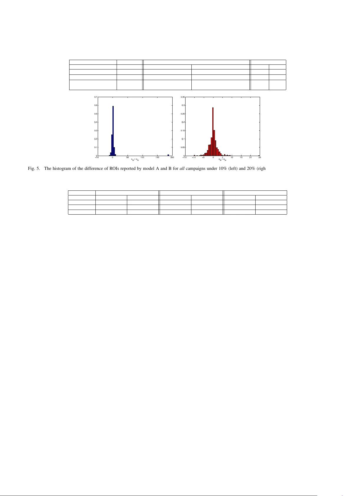
Online Model Ev aluation in a Lar ge-Scale Computational Adv ertising Platform Shahriar Shariat T urn Inc. Redwood City , CA Email: sshariat@turn.com Burkay Orten T urn Inc. Redwood City , CA Email: borten@turn.com Ali Dasdan T urn Inc. Redwood City , CA Email: adasdan@turn.com Abstract —Online media pro vides opportunities f or marketers through which they can deliv er effective brand messages to a wide range of audiences at scale. Advertising technology platf orms enable advertisers to r each their target audience by deliv ering ad impressions to online users in real time. In order to identify the best marketing message for a user and to purchase impressions at the right price, we rely hea vily on bid prediction and optimization models. Even though the bid prediction models are well studied in the literature, the equally important subject of model evaluation is usually overlook ed or not discussed in detail. Effective and reliable evaluation of an online bidding model is crucial for making faster model impro vements as well as for utilizing the marketing budgets more efficiently . In this paper , we present an experimentation framework f or bid prediction models where our focus is on the practical aspects of model ev aluation. Specifically , we outline the unique challenges we encounter in our platform due to a variety of factors such as heterogeneous goal definitions, varying budget requirements across different campaigns, high seasonality and the auction-based en vironment f or inv entory purchasing . Then, we introduce return on in vestment (ROI) as a unified model perf ormance (i.e., success) metric and explain its merits ov er more traditional metrics such as click-through rate (CTR) or con version rate (CVR). Most importantly , we discuss commonly used ev aluation and metric summarization approaches in detail and propose a more accurate method f or online ev alua- tion of new experimental models against the baseline. Our meta- analysis -based approach addresses various shortcomings of other methods and yields statistically robust conclusions that allow us to conclude experiments mor e quickly in a reliable manner . W e demonstrate the effectiveness of our evaluation strategy on real campaign data through some experiments. I . I N T RO D U C T I O N Advertisers are increasingly exploiting online media to reach target audiences through different channels such as search, display , mobile, video and social advertising. Similar to other forms of marketing, the ultimate goal is to deliv er brand messages to the most receptiv e set of users who are likely to con vert by taking a desired action after they are subjected to a particular type of ad impression. Even though the definition of a satisfactory outcome is advertiser dependent, identifying a ‘likely-to-respond’ user in real time is common to all online advertising campaigns. The real-time requirement comes from the fact that a significant chunk of ad impressions (i.e., the opportunity to serve an ad to an online user on a particular publisher page) are sold in marketplaces through auctions held by sev eral ad exchanges [1]. Real-time biding exchanges (R TBs) solicit the a vailability of an ad impression to all interested parties, such as the advertisers themselves or demand side platforms, like T urn Inc., who manage the advertisers’ campaigns on their behalf, and each impression is sold to the highest bidder . Finding the right set of users in this setting requires complex statistical approaches that accurately model user intent and optimize the bid price for every ad impression of each adv ertiser . Bid prediction models are at the heart of any advertising technology platform and they need to be enhanced in order to adapt to the evolving requirements of marketers and to remain competitiv e in a highly dynamic ad marketplace. In other words, new models need to be introduced or the predictiv e power of the existing models has to be improved continuously . A common first step towards quantifying the ef ficacy of a ne w model compared to a baseline is to carry out offline analysis and study the metrics that measure the predicti ve accuracy such as relative log-likelihood, area under the curve (A UC) and classification accuracy [2] or employ more sophisticated techniques such as contextual multi-armed bandits [3]. Even though of fline analysis provides helpful guidance, it does not capture the true performance of a bid prediction model, which needs to operate in a dynamic auction en vironment where the cost of impressions plays a significant role. No matter how positiv e the outcomes of the offline experiments are, we need to ev aluate the real (i.e., online) performance of a new model on li ve traffic and on real users in a controlled manner . Online ev aluation of a model in our platform is not a trivial task and we need to ensure that our experimentation and ev aluation framew ork is able to: • handle traffic allocation to both the baseline and experimental models, • allow dynamical contr ol of traffic allocation such that the models do not influence each other, • clearly identify a performance evaluation metric which aligns with the advertiser performance expec- tations as well as business value, • and, most importantly , enable model ev aluation in a complex, dynamic and heterogeneous auction environ- ment such that we can make quick progress tow ards deciding whether to replace the baseline model with the experimental one or not. Since an algorithmic change in a model affects the be- havior of the system we need to consider its impact on ev ery advertiser and make sure that we statistically improve the performance of a quite significant portion of our clients. Other works in the area of online advertising focus on the experimental design of single test [4], [5]. Howe ver , our problem is to design a frame work that can reliably and robustly summarize the effect of an improv ement in our bid prediction models. W e need methods and apparatus that can help us study the effect of a treatment applied to sev eral experiments and summarize them in a principled manner . In statistics literature, meta-analysis provides the basic tools and techniques for such task [6], [7], [8]. In this paper, we present a frame work that we utilize for online e v aluation of bid prediction models in our platform. W e outline the important components of our frame work, that are critical for conducting multiple model experiments at a very large scale such as user-based traf fic allocation, dynamic traffic control and budget management across dif ferent models. W e focus on the definition of a performance metric and the model ev aluation criteria. More specifically , we identify r eturn on in vestment (ROI) as the most suitable e valuation metric in our setting due to its alignment with both performance and business expectations. Then, we describe our meta-analysis- based model e valuation approach, which is robust to outliers and allows us to make more consistent decisions about the online efficac y of a model. The paper is organized as follows. W e first, in § II, describe the necessary background on the ad selection problem and the complications of a large-scale adv ertising platform. Then in § III, we detail the structure of our experimentation plat- form and its necessary elements. § V presents our ev aluation methodology and § VI studies a practical experiment. W e finally conclude this paper by § VII. I I . B A C K G RO U N D A demand side platform, manages marketing campaigns of sev eral advertisers simultaneously by identifying the tar get audience matching the campaign requirements and making real-time bidding decisions on behalf of the advertisers to purchase ad impressions at the ‘best’ price. In this section, we briefly describe rele v ant background information on some important aspects of online campaign management in our platform, which will set the stage for our model e valuation framew ork. A. Bid Pr ediction in A uction En vir onment Majority of the ad impressions in the online setting are sold through R TBs as we briefly explained in § I. These real- time decisions are made in response to what are called ad call requests from R TBs. Ad requests come to our system (essentially) in the form of ( user, pag e ) . Here we use pag e to represent the media on which the ad will be served (e.g., a webpage, mobile app or a video player). The main purpose of ad selection is to identify the most relev ant match among all qualifying ads. Let A = { a 1 , a 2 , ..., a m } denote the set of all activ e ads in our system. Identifying the best ad entails finding the ad with the highest bid price for the incoming request: ad ∗ = arg max k =1 ,...,m B id ( a k ) (1) Bid price of each ad is a function of campaign parameters and the desired outcome that each marketer is trying to accomplish. Some campaigns are tailored for pure branding purposes rather than expecting a direct response from the user and in this scenario, advertiser usually resort to a fixed bid price. In other words, bids are not dynamically adjusted for each request. Howe ver , the more common scenario is to hav e a performance goal associated with the campaign and optimize the bid price at each request to maximize the likelihood of getting a desired ‘outcome’ once the ad impressions are served to online users. Bid estimation in this case in volv es utilizing machine learned models [9], [10] to estimate the likelihood of the desired ev ent and bid for a k can be computed as: B id ( a k ) = Goal ( a k ) ∗ p ( outcome | user , pag e, a k ) (2) where Goal ( a k ) is a target value that is assigned by the advertiser at the beginning of a campaign and outcome is one of a click, a con version, a view , etc. Intuitiv ely , this computation captures the expected value of an impression to a particular advertiser . Collectiv ely , we refer to the system that is capable of 1) estimating likelihoods, 2) computing bids for v arious types of ads and 3) ranking them according to business and performance objecti ves as the bid prediction model . After we select the best ad internally , we submit a response to the exchange where a secondary auction is held among all participants to identify the winning ad to be served to the online user . W e should emphasize that R TB auction is held independently and our internal bid prediction models are required to handle the price uncertainty associated with a very dynamic external marketplace. B. V arious Campaign Goals As we briefly touched upon in § II-A, the overall bid prediction system and bidding models are highly dependent on the outcome event advertisers are interested in and the goal v alue they associate with that ev ent. This outcome could simply be the user clicking on the served ad or it could be a more direct response such as a con version ev ent (e.g., signing up for a newsletter , requesting a quote or purchasing an item) as identified by the marketer . In other words, we need to keep track of multiple e vent types (clicks, con versions, engagement, view ability of the ad etc.) and their respective value for each adv ertiser . While this custom setup gives a lot of flexibility to accomplish v arious marketing objecti ves, it results in a highly heterogeneous en vironment for the optimization platform to ev aluate. Commonly used metrics such as click- thr ough rates (CTR), con version rates (CVR), cost-per-click (CPC) or cost-per-con version (CPCV) do not fully capture the global performance of our bidding models. For example, as we try to improve the CTR-based performance, we sometimes find ourselves hurting the CVR metric for some campaigns or the av erage cost of conv ersions may go up. Model experimentation in this environment requires a unified (i.e., normalized across campaigns) goal definition that we can rely upon to quantify and assess the o verall model performance. C. Seasonal and V arying Budgets In addition to the target audience a campaign is trying to reach, two other factors that play a crucial role in a campaign’ s final outcome are the duration of the campaign (i.e., flight time) and the total allocated budget. Depending on the time of the year , a vailability of a product to be promoted or their business strategy , marketers modify campaign goals !"#$"%&'() *"+,-) .-'-/"0-1) 23-/"++) 4$-'1%'&) 5-0,/')6')7'3-(0#-'0)85279) ! :) *"+,- ;<:) 4$-'1 ;<:) 527 ;<: =*"+,- ;<: >4$-'1 ;<:) ! ?) *"+,- ;4$-'1 ;4$-'1 ;<@) A) A) A) A) ! ') *"+,- ;<') 4$-'1 ;<') 527 ;<' =*"+,- ;<' >4$-'1 ;<') B61-+);C)D"#$"%&')+-3-+)(0"E(ED()) B61-+)FC)D"#$"%&')+-3-+)(0"E(ED()) !"#$"%&'() *"+,-) .-'-/"0-1) 23-/"++) 4$-'1%'&) 5-0,/')6')7'3-(0#-'0)85279) ! :) *"+,- F<:) 4$-'1 F<:) 527 F<: =*"+,- F<: >4$-'1 F<:) ! ?) *"+,- F4$-'1 F4$-'1 F<@) A) A) A) A) ! ') *"+,- F<') 4$-'1 F<') 527 F<' =*"+,- F<' >4$-'1 F<') Fig. 1. Important campaign statistics used in model A/B experiment. Both models A and B deliver impressions for n campaigns and the resulting R OI statistics are combined to make an overall model assessment. and budgets continuously . At any giv en time, we hav e in our platform sev eral thousand campaigns activ e that have competing goals as well as highly v arying budgets. Disparity between the budgets of a small campaign and a larger one can easily reach a factor of 1000s. Since our bidding models are simultaneously optimizing the campaign performance ov er the whole ecosystem, composition of different types of campaigns we are running, their goals and respective budgets play a fundamental role in our model e valuation. In other words, our ev aluation approach has to take into account all these factors while making a final decision on the outcome of an online experiments. I I I . E X P E R I M E N T P L A T F O R M S E T U P Offline experimentation and ev aluation using classification or ranking metrics is a commonly used initial step to wards improving a bidding model. Howe ver , we hav e experienced multiple times in v arious experiments that offline success does not necessarily indicate positive outcomes in liv e traffic and finding correlations between offline and online results is an ongoing area of research (cf. [11]). This is particularly , due to lack of access to the exchange’ s logs and therefore, the inability to accurately simulate the external auction. Further- more, for practical reasons, the logs typically cannot contain the data for all bid-requests and only the portion that are won by the DSP is kept. The most commonly used approach for online ev aluation is A/B testing, which is a randomized experiment where a ne w tr eatment model, referred to as B , is being e valuated against a contr ol (or baseline) model, referred to as A . The goal is to compare the ef ficacy of a treatment model B over the control A on a statistically identical population by measuring the difference in an overall evaluation criteria of interest on (dynamically adjustable) online user traffic . Running controlled online experiments at internet scale is an interesting problem by itself (cf. [4], [5]) but a detailed description of such an experimentation platform is beyond the scope of our paper . Instead our focus in this section is to highlight the most important aspects of our online experimentation platform as it pertains to our specific needs of ev aluation for bidding models. A. Online T raffic Allocation The success of a randomized experiment heavily relies on a proper split of the samples over which the control and treatment models will be evaluated. In our context, one may consider allocating the incoming liv e (request) traf fic randomly to one of the bidding models and let the chosen model handle the selection of the best ad from one of the activ e campaigns as well as the proper choice of a bid price. Howe ver , this randomization scheme would ignore the user component of a bid request completely and would result in both the control and treatment model serving impressions to the same user . Subsequently , it would be difficult to identify the actual causal impact of a model in case of a successful outcome such as a con version. In order to minimize the impact of models over each other, a user-based traffic split is best suited for our A/B testing purposes [12]. More explicitly this corresponds to pre-allocating a subset of users to the treatment (i.e., B ) model such that any time we recei ve a bid request from any R TB for this user, ad selection and bid prediction will always be handled by model B and the rest of the requests will be directed to the baseline model A . After deciding on how to allocate the incoming online traffic to models, the next decision to make is how much traf fic to actually allocate to the treatment model. In an ideal A/B testing scenario, user sample would be split equally at A : %50 , B : %50 . Since the li ve e xperiments are conducted in a production en vironment while the campaigns are activ e, system health and campaign performance requirements can potentially be jeopardized if a model exhibits unexpected behavior with high traf fic. It is much safer to acti vate the treatment model on a small percentage of users initially and ramp up the traffic as we collect e vidence indicating that the experimental model is performing better then the control. For example, one can decide to adopt the following schedule while running a model e xperiment: Online Experiment Schedule Phase 1 T raffic allocation: A : %99 , B : %1 , duration: 1-2 days Online Experiment Schedule Phase 2 T raffic allocation: A : %90 , B : %10 , duration: 1 week Online Experiment Schedule Phase 3 T raffic allocation: A : %80 , B : %20 , duration: 1 week Online Experiment Schedule Phase 4 T raffic allocation: A : %50 , B : %50 , duration: 1 week Actual traffic percentages and the duration of each phase should be selected such that sufficient evidence is collected ov er all representative entities in the e xperiment. In our plat- form, e ven though our ultimate goal is to make a model-level assessment, we consider ev ery active campaign as a separate experiment under the new model (see Fig. 1). Therefore, we need to tune the traf fic share and the duration of the experiment such that the majority of the campaigns can collect suf ficient number of users to exhibit enough statistical power [12]. W e should emphasize that treating each campaign as an individual experiment is a very fundamental aspect of how we approach online model ev aluation. Recall from § II that every campaign object is identified by a dif ferent target audience, flight time, optimization goal and a monetary budget. Gi ven this variabil- ity , treating various types of activ e campaigns while running experiments requires a meticulous ev aluation methodology so that we are able to make statistically reliable and robust conclusions. W e should also point out that the campaign le vel assessment approach we will outline does not change how we split and allocate the online traffic based on user IDs. Since the rate at which we receiv e queries from multiple R TBs in our platform is very high (˜ 2 . 5 million bid requests per second as of this writing), with a high enough traf fic percentage and a reasonably long experiment (e.g., 2-3 weeks) majority of our activ e campaigns get to observe sufficient number of requests from many users. In other words, uniform random split criteria yields a good (i.e., representati ve) sample for both models A and B under each campaign such that not only can we make individual assessment at the campaign lev el, but we can also make a statistically reliable decision for the overall performance of a bidding model. B. Overall Evaluation Criteria Another important component in an online experiment is the pre-determined over all evaluation criteria (OEC), which will be used to determine ev aluation outcome. Even though it is possible to track multiple metrics during a large scale experiment to gain insight into the performance of a model from different perspectiv es, OEC should be identified as the ultimate metric that both captures the statistical properties of our models and also aligns well with the business success. As we discussed in § II-B, flexibility in defining custom campaign goals makes it a challenge for us to compare the impact of a new bidding model across thousands of activ e campaigns. As an example, our bidding algorithm might be positiv ely impacting (i.e., reducing) the cost of con version for a con version optimizing campaign whereas a click optimization type campaign might be observing an inferior CTR within the same time period. Our aim is to define a unified metric that will simultaneously capture the performance of ev ery type of campaign which is adaptive to their custom defined goal types. Before we define our choice of OEC metric, we first hav e to introduce the concept of a value that each campaign may get to observe after each ad impression is served. Recall that campaigns can be tracking v arious types of events such as clicks, con versions or ad views. Adv ertisers define a goal value that they associate with the ev ent they are optimizing tow ards. Based on the event type and the monetary v alue they associate with the ad, we can define whether they generated value as a result of an impression or not. For example, if the target ev ent is a click, which has been valued at $0 . 5 , and if the campaign generates 1000 clicks after a period of time, we can conclude that $500 worth of value was generated within that campaign period. Then, for campaign i which is tracking e different types of ev ents valued respectiv ely at v alue 1 , v alue 2 , ..., v alue e ov erall value generated after spending a b udget of spend i can be computed as: V alue i = X k =1 ,...,e v alue k ∗ (# of events of type k ) (3) In other words, we can say that campaign i generates a total V alue i as a result of in vesting S pend i in ad impressions. Then we can define the overall success level of a campaign in terms of r eturn on investment (R OI): RO I i = V alue i S pend i (4) Unlike the other ev ent specific metrics such as CTR, CVR, CPCV , etc., ROI provides a normalized performance metric that unifies the overall success level of any type of campaign reg ardless of their target event. ROI is our choice of OEC for our online bidding model experiments and we will demonstrate in the section below how it can be used for A/B test ev aluations. C. Evaluation Setup Definitions & Notation Having discussed the traffic split and OEC in detail in previous section, we would like to outline all important quantities we measure at the campaign lev el that will be used for ov erall model ev aluation. Note that we use online experiment and A/B test interchangeably and they both refer to the randomized experiment we conduct in a production en vironment on li ve bid request traffic. Listed below is our notation and the definition of relev ant quantities we will be using in § IV (also see Fig. 1). • i=1,...,n: index that identifies different campaigns which are active during an online experiment • A : baseline model currently used in production • B : experimental model we are e valuating against A • M ∈ { A, B } : indicates a model, A or B • S pend M ,i : T otal spending of campaign i by model M • V alue M ,i : T otal value generated for campaign i by model M after spending S pend M ,i during the experiment • RO I M ,i = S pend M,i S pend M,i : ROI of campaign i observed by model M The overall ev aluation pipeline is illustrated in Fig. 2. Note that the traffic increase to a model might need the approv al of a manager who has to weigh the estimated improvement caused by the model against its computation cost and other consid- erations. Particularly , for this purpose we need an evaluation method that gives a reliable impr ovement amount . Before we conclude this section, we should reemphasize that campaign lev el R OI is a core element of our ev aluation method where !"#$%&'&()*+$ ,*-&'$!$ . / $ ,*-&'$!$ . + $ ,*-&'$#$ ,*-&'$#$ . / $ . + $ 012'32)*+$,&45*-$ !((&647$ %89:$ ;+(<&2=&$4<2>($ 4*$#$$ ?@ !"#$ A$62B&C?$ D0%$ E9$ Fig. 2. The overall pipeline of the evaluation platform. W e increase the traffic to the treatment model until it becomes dominant and replaces the baseline. The traffic increase might be subjected to the approv al of a manager . each campaign’ s spend and R OI statistics under each model are treated as an individual experiment and the final outcome is based on a robust combination of individual ROIs. The next two sections we mention different ev aluation designs that we hav e considered and describe our proposed and final approach in detail. I V . E X I S T I N G E V A L UAT I O N D E S I G N S The problem is to design an e v aluation method that can quickly and reliably reject or accept a new model for assigning more traffic. Moreover , we would like to gain as much insight as possible into the performance of the proposed models. Furthermore, the e v aluation method must be able to estimate the expected amount of improvement. Micro-a veraging (Micro) : This is a conv entional summa- rization technique in data mining and information retriev al [13]. Based on this method, W e define the R OI of the model as RO I M = P n i =1 V alue M ,i P n i =1 S pend M ,i (5) Note that (5) can be written as RO I M = n X i =1 S pend M ,i P n i =1 S pend M ,i V alue M ,i S pend M ,i , (6) which is the weighted av erage of the ROI of each campaign (for each model) by its spend. The final decision using this method is made based on the dif ference of two computed R OIs. That is, µ M icr o = RO I B − RO I A (7) and we require µ M icr o > θ , where θ can be set using an A/A test [12]. A/A test :T o decide on θ , we randomly divide the data (bid requests) of each campaign observed by the control model (A) into two non-ov erlapping subsets, A 1 and A 2 , proportional to the size of A and B and compute µ M icr o A/ A = RO I A 1 − RO I A 2 as if the subsets were two models. Since the two subsets are created from the same model, a non-zero µ M icr o A/ A can be ascribed to the system v ariation. W e repeat this task K times (5 in our experiments) and we set θ = 1 K P K k =1 µ M icr o ( A/ A ) k . Note that the A/A test accounts for the variation of the whole system rather than for each indi vidual campaign. First, it must be noted that our objective is to improve the performance of as many campaigns as possible while obtaining a better global picture. In other words, if we observe a global advantage such that a few large campaigns experience very large improvement in their metrics while many other campaigns suf fer from a degradation, then we must conclude that the model is not significantly better, compared to the control. This method naturally gi ves more weight to the higher spending campaigns. In § VI we will demonstrate how this can be a dangerous property . Macro-a veraging (Macro) : Another con ventional data mining method closely related to Micro-av eraging is Macro- av eraging. It is essentially the average of the differences of metric over campaigns. That is, µ M acr o = 1 n n X i =1 ( RO I B ,i − RO I A,i ) . (8) The final decision using this method is that we accept the model if µ M acr o > θ , where θ is determined using an A/A test analogous to Micro-a veraging. This method has the advantage of considering the perfor- mance of the treatment model equally over all campaigns. The obvious shortcoming of this method is its sensiti vity to the outliers. A large dif ference between the performance of the two models can happen due to the traf fic split especially for small campaigns. This can result in an undesirable skew in the measure. Another disadvantage of this method is consid- ering an y dif ference without accounting for the variation and sampling error within and between the campaigns. A plausible solution for reducing the sensitivity to outliers is to use median instead of average. Ho we ver , since we usually hav e many campaigns, the median and av erage are not far different from each other . In our experiments we rarely noticed a difference between median and average such that it results in contrasting decisions. Other outlier remov al and noise reduction techniques are also not suitable since remov al of any of the campaigns from the analysis might result in a biased decision making. One needs to weigh different measurements based on their reliability and then combine them. Summarized statistical analysis : There are two possible methods for summarizing the statistics of the effect of the treatment model: i ) One can compare the distrib utions of the RO I A,i and RO I B ,i ov er all campaigns using a statistical test such as K olmogorov-Smirnov (K-S) or other fitting tests [14]. Such tests, again, ignore the v ariation inside each e xperiment and also do not result in an o verall improv ement measure. ii ) T o account for the variation within each campaign one can use a statistical significance analysis such as a Student-t test [14] by considering the distribution of the measurements within each campaign. This method howe ver , still leav es us without a wholesome measure of improvement. Also, since we conduct the tests on a pretty lar ge set of campaigns, we need to deal with the family-wise error and false discov ery rate issues[15], [16]. Another disadvantage is that this approach leaves the insignificant campaigns out of the analysis while this is not desirable. W e need a method that systematically accounts for the v ariations and combines the statistics of all campaigns according to that. Meta-analysis provides us with such tools. W e describe the detail of our adaptation of meta-analysis in the next section. V . P R O P O SE D M E TA - A NA LY S I S Meta-analysis enables us to combine our estimates of the difference of the control and treatment models over multiple campaigns. In this section, we describe the methodology that provides us with a global estimate based on which we decide whether to reject the model or increase its traffic share. W e divide the traffic that is received by each model into sev eral parts based on the user ids or uniformly at random . Each part, for instance, can correspond to 1% of the traffic directed to the model. T o this end, assume that models A and B receive m A and m B parts of the traffic, respectiv ely . Also, to simplify the notation we denote the measurement (ROI in this case) of the j th part of the i th campaign by R A,i,j and R B ,i,j for models A and B , respectiv ely . The parts might needed to be excluded from the analysis due to insufficient number of impressions as a pre-processing procedure. One such procedure is described in § VI. A. Effect size The effect size of a test is a (standardized) measurement of the difference between the means of the two sets of samples [6]. This gives us an estimate of how the distrib utions of the two sets (assuming a normal distribution) differ . Assuming that one set of samples belong to our treatment and the other is the result of applying the control, the effect size can estimate ho w much better or worse a treatment model is compared to the control. Combining these effect sizes can provide us with a global picture of the performance of the treatment. In statistical modeling three major types of models are considered. Fixed, random and mixed effect models. Fixed effect model assumes that the effects are the same in all tests and the difference between them is only caused by sampling error . In contrast, the random model assumes that the variation is systematic and the effects are sampled from a distribution related to the structure of the tests. A mixed model, obviously , assumes a mixture of the two. W e assume a random effect model because the variation between campaigns can be explained by assuming a latent distrib ution gov erning the local and global auctions and the inherent structure of the campaigns themselves. W e start with the fixed effect model to calculate the ef fects and their corresponding v ariances and then expand to the random ef fect model by computing the between-variance of the ef fect sizes. Let ¯ R M ,i and s 2 M ,i be the sample average and variance of R M ,i, · ov er all acceptable parts of the model M for campaign i . The effect size is the normalized dif ference of the means of the two distributions. Therefore, assuming a normal distribution over the measures, ROI of each part in our case, the standard effect size of the i th experiment 1 is defined as δ i = ¯ R B,i − ¯ R A,i s p i , where s 2 p i = ( m A − 1) s 2 A +( m B − 1) s 2 B m A + m B − 2 1 W e will use experiment or study and campaign interchangeably . is the pooled variance of R A,i, · and R B ,i, · distributions. The pooled variance is the weighted average of the sample variances of the two populations such that the weights are their sizes. The assumption is that both populations share the same variance but their means might be different [8]. Note that δ i follows a noncentral Student-t distribution with d f = m A + m B − 2 degrees of freedom and noncentrality parameter , δ [17]. Therefore, for each campaign, the unbiased effect size (mean of the distribution) is d i = c ( d f ) δ i , where c ( d f ) = 1 − 3 4 d f − 1 . The corresponding v ariance of the ef fects is also the variance of the noncentral Student-t distribution v i = c ( d f ) 2 ( m A + m B m A m B + d 2 i m A + m B ) . For a comprehensiv e dis- cussion on the ef fect sizes refer to [18], [6]. Note that the variance is at its minimum when m A = m B . Also, note that the variance is quadratically related to d . There- fore, when the allocated traffic to the treatment model is much smaller than the control, the v ariance is high. Similarly , when the ef fect itself is lar ge, our uncertainty about its accurac y is high. The next step is to combine the effects. W e approximate the noncentral Student-t distribution of the effects by Gaussian. Furthermore, it is reasonable to assume that the experiments are mutually independent since the campaigns do not share ads or budget. The total effect can be summarized by the weighted av erage of the effects of each individual experiment. That is, T = n X i =1 β i U i , (9) where U i ∼ N ( d i , √ v i ) and T ∼ N ( µ, √ ν ) . Note that µ = P n i =1 β i d i and ν = P n i =1 β 2 i v i . It is straightforward to observe that setting β i = 1 / v i P n i =1 1 / v i minimizes the variance (uncertainty) of T , subject to β i > 0 and P n i =1 β i = 1 [18].Therefore, letting w i = 1 v i , one could sho w that the total mean effect size and variance are µ = P n i =1 w i d i P n i =1 w i and (10) ν = 1 P n i =1 w i , (11) respectiv ely . Equation (10) is intuitiv ely an appropriate esti- mator of the summary effect for us since it accounts for the variation inside each e xperiment and weighs them based on our uncertainty about their effect sizes. Furthermore, (11) accounts ev en for the traffic directed to the treatment such that the total variance is higher for more unbalanced traffic allocations between treatment and control. Now , we need to study the possible v ariation between the studies and test our assumption of a random model. Namely , we need to test whether the variation of the effects are due to sampling or there might be an underlying distribution causing such variation. The homogeneity statistics, Cochran’ s Q [19], is the appropriate and con ventional homogeneity test, which addresses this question. The null hypothesis is that all effect sizes are the same and the observed v ariation is only due to sampling error . Cochran’ s Q , Q = i = n X i =1 w i ( d i − µ ) 2 , (12) Fig. 3. The steps for making a decision by our method. Subgroup analysis might be omitted where a ’ strong’ rejection is suggested by the method. is distributed as χ 2 with n − 1 degrees of freedom. Therefore, p Q = 1 − χ 2 ( Q, n − 1) defines the p-v alue of the homogeneity . This is an important metric that shows whether we are facing a homogeneous set of ef fects or not. A homogeneous effect is rather desirable since it stands for a steady and explainable effect over all tests. It means that the effects have enough ov erlap that we can safely say that the difference between them looks like to be the result of sampling and the model affects all the tests roughly in the same way . W e no w compute the statistics of the random effect model. Herein, we assume that the effect sizes are sampled from a normal distribution T between ∼ N (0 , τ ) . The variance of this distribution is defined by τ 2 =  0 Q < ( n − 1) Q − ( n − 1) λ other wise (13) where Q is gi ven by (12) and λ = P n i =1 w i − P n i =1 w 2 i P n i =1 w i . The abov e is based on the simple method of moments [7], which is the most popular method to compute τ 2 . Based on the random model, we are assuming that U ∗ i = U i + T between , where U ∗ i ∼ N ( d ∗ i , v ∗ i ) , where d ∗ i = d i and v ∗ i = v i + τ 2 . Consequently , w ∗ i = 1 v ∗ i . Therefore the total effect is T ∗ ∼ N ( µ ∗ , ν ∗ ) where µ ∗ = P n i =1 w ∗ i d i P n i =1 w ∗ i and (14) ν ∗ = 1 P n i =1 w ∗ i . (15) The abov e approach is rather rob ust to outliers since it assigns a smaller weight to those campaigns that report abruptly high or low effect sizes. Furthermore, the variance of the estimation can gro w if the effects are widely spread. These are exactly the properties that we were seeking for our estimation of the ov erall effect of a treatment model. That is, the outliers are systematically downgraded based on their uncertainty and the variation between the ef fects is also tak en into account. The null hypothesis that the summary effect is zero can be tested using a Z-v alue such that Z = µ ∗ √ ν ∗ . (16) Particularly , the effect is significant if ( P z = (1 − φ ( | Z | ))) < α 2 , where φ − 1 ( · ) is the in verse cumulative distrib ution function of the normal distrib ution. The confidence interval [14] for the confidence lev el α is defined as C I = [ µ ∗ − φ − 1 (1 − α 2 ) √ ν ∗ , µ ∗ + φ − 1 (1 − α 2 ) √ ν ∗ ] . (17) The primary decision for accepting or rejecting the treatment model is based on the abov e significance test and the confi- dence interval. Based on the purpose of the model and the allocated traffic, we require a certain lev el of significance for the ov erall ef fect to be accepted. The significance le vel can be adjusted using an A/A test as described in § IV. Furthermore, the confidence interval gives an estimation of the expected improv ement. Usually , we require a smaller significance level when the traffic share of the treatment model is smaller . The sequence of the decision-making for the proposed ev aluation method is illustrated in Fig. 3 B. Subgr oup analysis It is necessary , in many cases, to explain the effect of the model on a subset of campaigns and then study the relationship between them. F or instance, we might need to kno w ho w the model affects the high spending campaigns or those that seek a con version or click goal. Furthermore, one is usually interested in understanding the variation inside and between subsets or groups. Particularly , we are interested in observing whether or not the group membership can explain the variation among the effects. The analysis of the variation amounts to analysis of Cochran’ s Q for different groups, which is typically referred to as subgroup analysis in the literature [6]. Let G = { g 1 , · · · , g K } be the set of subgroups such that S K k =1 g k = { C 1 , · · · , C n } and g k ∩ g k 0 = ∅ ∀ k , k 0 ∈ { 1 , · · · , K } , k 6 = k 0 . One then, can compute Q ∗ k using a formulation similar to (12) modified so to use the summary effect and weights of the random model. Essentially , we want to study the homogeneity of the effects around the mean within each subgroup. That is, Q ∗ k = X C l ∈ g k w ∗ j ( d l − µ ∗ k ) (18) where µ ∗ k is the summary effect of the random model for the k th subgroup. The total Q ∗ is also computed ov er all studies giv en the total mean effect, which in turn represents the devia- tion from the grand mean. No w , we would like to test whether the total heterogeneity of the studies can be explained by aggregating the heterogeneity of all subgroups.Remembering that Q follows a χ 2 distribution, we define Q ∗ within = X g k ∈ G Q ∗ k . (19) Finally , if the summation of the homogeneity statistics was able to explain the total homogeneity , one might conclude that there is no considerable variation between the groups and thus the group membership does not define the beha vior of a giv en campaign. T o represent that, the variation between the subgroups can be calculated as Q ∗ between = Q ∗ − Q ∗ within (20) and tested for significance with the null hypothesis that the group membership does not af fect the effect sizes. Q between has K − 1 degrees of freedom. The same study can be done in a hierarchical fashion to study larger subgroups [6]. Using the abov e approach, it is possible that we find model B to be effecti ve only in certain cases. For instance, the campaigns that have a very low budget might benefit from the properties of the proposed model. In that case, we might decide to add B to our stock of models and apply per business requirements. V I . C A S E S T U DY The purpose of the this study is to sho w that our proposed method 2 is able to arriv e at a robust and consistent decision using a smaller portion of the traffic compared to other methods. It is intuitive that a more reliable comparison can be achieved when the treatment model receiv es more traffic. Therefore, a good measurement mechanism is the one that arriv es at a decision that does not change as we increase the traffic directed to the treatment model. Essentially , we demonstrate that our meta-analysis-based approach points to a decision in the first step of the analysis while other methods need more traffic (samples) to arrive at the same decision. In this case study , we are studying the ef fect of a change that affects a primary part of our prediction algorithm. The model will be applied to the campaigns that intend to serve ads on mobile de vices. The hope is to observ e a significant increase in the ROI of the whole system. T o comply with company policies we refrain from sharing the absolute numbers and restrict ourselves in reporting only relative results. The number of campaigns that are studied is about a thousand. W e use a noise remov al procedure before applying our ev aluation method. W e require each part to contain a minimum number of impressions (100 in this experiment) and if it does not, then we remov e that specific part from the analysis. If the number of removed parts for each model exceeds 10% of the total parts of each model, then the whole campaign is disqualified. Essentially , the number of qualified parts for model A and B must be more than 0 . 9 m A and 0 . 9 m B , respectiv ely so that the campaign is included in the analysis. This means that tests might have different sizes depending on how much b udget they hav e and how many users they can reach. W e observed that only 0.5% of the campaigns were disqualified as the result of this pre-processing. T o be fair to other methods we apply them to the same set of campaigns. Setting 1: T wo e xperiments are conducted to observe the robustness and correctness of the decision-making procedure by each method. The experiments differ in the traffic share that the treatment model receiv es and in the time period in which they were running. In particular, in the first experiment the treatment model receives 10% while control recei ves the rest 2 The code and a sample data set is av ailable at https://github .com/turn/ModelEvaluation ✲  ✁ ✲  ✂ ✲ ✁ ✂ ✁  ✂  ✁ ✷ ✂ ✷ ✁ ❙ ✄ ☎ ✆ ✝ ❘ ❇ ✞ ✟ ✥ ❘ ❆ ✞ ✟ Fig. 4. The difference of R OIs of the two models vs the spend under 10% (blue) and 20% (red) traffic for ev ery common campaign between two experiments. The spend is the total spend of the campaign summing up over both models. A few high spending campaigns with slightly worse situation causes the Macro method to change its decision. of the traffic and it runs for 12 days. The second experiment runs right after the first experiment for 10 more days but the treatment model receiv es 20% of the traffic. In this setting, we constrain ourselves to the common campaigns in both experiments and make sure that their setup (budget, targeting, etc.) is not changed between the two time periods. In other words, the campaigns that are under study will be limited to the intersection of the two sets of campaigns that were present in both experimentation periods and also pruned for identical setup. This constraint removes nearly 32% of campaigns from the union of the two sets of campaigns. Most (98.4%) of the remov ed campaigns are the ones that did not e xist in the first experiment. The rest of the removed campaigns, mainly , had budget changes. The whole experiment runs over a period of one month to make sure the seasonality does not af fect our results substantially . This approach will allow us to observe the robustness of the decision that is made by each method giv en the increased traf fic. The parameters of each method is estimated based on an A/A test as described in § IV. There was almost no change in the computed parameters between 10% and 20% traf fic. The results are depicted in T ab . I. T able I reports the statistics of each method given the parameters and the decision for accepting or rejecting the treatment model based on them. It is evident from the results that Macro and Micro methods changed their decision with very drastic drop in their statistics after the traffic was increased to the treatment model. The proposed method howe ver , suggests to reject the model in both experiments. Essentially , in both e xperiments we observe that the Z-test accepts the null hypothesis that the model has no effect. Ev en though in the second experiment the confidence interval is more towards the negativ e effect, it is not significant giv en the required significance le vel. Even if we declare the summary effect significant by reducing the significance level, the confidence interval still suggests a reject. Figure 4 illustrates the difference of the R OIs of the control and treatment models for the two traffic settings for each campaign versus its total spend. Each dot represents a campaign. The blue dots stand for 10% and red ones for 20% traffic designation to the treatment model. W e hav e remov ed the numbers in the x-axis to comply with company’ s policies but obviously the right most dots represent the highest T ABLE I. R E SU LT S O F A P PLY IN G EA C H M ET H O D O N C O M MO N STA B LE C AM PA IG N S Parameter Statistics Decision Treatment traffic 10% 20% 10% 20% Macro θ = 0 . 004 µ M acro = 0 . 17 µ M acro = − 0 . 05 Accept Reject Micro θ = 0 . 01 µ M icro = 0 . 29 µ M icro = − 0 . 31 Accept Reject Proposed Method α = 95% C I = [ − 0 . 02 , 0 . 01] C I = [ − 0 . 028 , 0 . 009] Reject Reject P Z = 25 . 7% P Z = 15 . 7% spending campaigns. Since we have pruned the campaigns for only those that are common between the two experiments and hav e no setup change, each blue dot has a corresponding red dot with almost the same x coordinate (spend). Note that many red dots are positioned below the blue ones. Some of them are in the right half of the plot, the highest spending campaigns. This explains why Macro and Micro changed their decisions after the traffic was increase. Micro considers a weighted av erage of the differences where weights are determined by the spend of each campaign. This makes this method particularly sensitiv e to the behavior of high spending campaigns (the right half) and thus its statistics dropped substantially after the traf fic increase. Setting 2: In the second set of experiments we apply the methods on all campaigns reg ardless of their presence in both experimentation time periods or their setup. The results are reported in T ab . II. Again, we observe the same trend. All competing methods report substantial drop in the measure and change in their decision while the proposed method suggests to reject the model in both cases due to ineffectiv eness. As in the pre vious setting, we did not observe any change in the parameters based on the A/A test. The success of the proposed approach lies in the way that it chooses to weigh the ef fect of each campaign and the fact that it considers the variations within and between the studies. It is important to note that we need to consider the outliers in our final decision making since they are still part of our system. The fact that the y ha ve served enough impressions while the treatment model had an extraordinary ef fect on them makes them interesting but does not allo w us to ignore them. Smaller traffic increases our uncertainty about the observed effect and also a large ef fect must be downgraded as it can be easily caused by sampling error . All of these intuitions are captured in the weighting mechanism of the proposed method. T o observe why Macro-av eraging changes its decision giv en the very same parameters, refer to Fig. 5. The reported histograms in Fig. 5 sho ws the distrib ution of the difference of the ROIs for all campaigns. Note that when the traf fic directed to the treatment is at 10% (left plot), the histogram is tilted tow ards positiv e differences of R OI with a very prominent outlier . Once the traffic is increased to 20% (right plot), the distribution becomes narro wer (smaller variance) and slightly tilts to wards the ne gati ve dif ferences. This results into a change of direction in the decision of the Macro methods. Micro-av eraging, as discussed in the previous setting, is susceptible to outliers when they happen to have high budgets. This property of Micro-av eraging, prev ents it to be fair to many campaigns that ha ve medium or lower budgets but it is also desirable in the sense that it brings some notion of business value into the analysis. In other words, the high spending clients tend to be more important from a business perspectiv e. T o add an analogy to our method, we resort to subgroup analysis, which studies the behavior of the treatment model in more depth. W e need to mention that the homogeneity test for all experiments failed to reject the χ 2 test with 10% significance lev el and thus, the ef fect was considered to be homogeneous ov erall (loosely speaking). T o study the importance of the spend (budget) on the variation of the ROI ef fect sizes, we proceed as follo ws: W e divide the campaigns into three subgroups based on their spend. W e sort the campaigns decreasingly by their spend and use the cumulative sum of the spend to divide them into subgroups. Subgroup 1 contains the highest spending campaigns that collectiv ely spend 33% of the total amount of the money spent by both models and subgroup 3 is comprised of the lowest spending ones. Subgroup 3 contains much more campaigns compared to the other two. The results are shown in T ab . III for both 10% and 20% traf fic shares and all running campaigns. The subgroup analysis rev eals that regardless of the budget, all campaigns suffer some degradation in the performance where P Q between = 8% is under 10% traffic and it decreases to 4% in case of 20% traffic, which is significant for a 10% significance lev el. This means that the group membership affects the variation of the ef fect size and the effect of the model on each campaign is dependent on the giv en budget. Note that subgroup 2 is more se verely af fected by the new model. Basically , from the subgroup analysis based on the spend we conclude that there is no benefit in applying the model to a certain group of campaigns and it is particularly harmful to medium b udget campaigns. In summary , the proposed approach enabled us to reject an ineffecti ve model in earlier stages compared to other methods and provided us with various insights into the behavior of the model in a concise set of statistics. W e observed how the treatment model af fected the ov erall performance of the system through robust and quantitativ e measurements. Furthermore, we studied its beha vior giv en a more similar set of campaigns through subgroup analysis and observed that its insignificant performance can only get worse for medium budgeted cam- paigns and there is no chance of obtaining any impro vement for any categories of spend. V I I . C O N C L U S I O N In this paper we presented a general framework that could reliably and consistently ev aluate a ne w model compared to a baseline for online bid prediction in a very large system comprised of di verse set of campaigns with variety of goals and budgets. W e described the challenges in this area and variety of practices and ideas that we had implemented to arriv e at the current system. Our system is able to ef ficiently and dynamically direct the online traffic to appropriate experi- mental and baseline models allo wing us to hav e a statistically sound randomization and thus ev aluation.Using the return of T ABLE II. R E SU LT S O F A P PLY IN G EA C H M ET H O D O N A L L C A M P A I G N S Parameter Statistics Decision Treatment traffic 10% 20% 10% 20% Macro θ = 0 . 001 µ M acro = 0 . 14 µ M acro = − 0 . 03 Accept Reject Micro θ = 0 . 005 µ M icro = 0 . 10 µ M icro = − 0 . 99 Accept Reject Proposed Method α = 95% C I = [ − 0 . 019 , 0 . 009] C I =  − 0 . 03 , 9 . 6 × 10 − 4  Reject Reject P Z = 24 . 2% P Z = 3 . 3% ✲  ✁ ✁  ✁ ✶ ✁ ✁ ✶  ✁ ✷ ✁ ✁ ✁ ✁ ✵ ✶ ✁ ✵ ✷ ✁ ✵ ✂ ✁ ✵ ✄ ✁ ✵  ✁ ✵ ☎ ✁ ✵ ✆ ❘ ❇ ✝ ✞ ✥ ❘ ❆ ✝ ✞ ✲  ✁ ✲  ✂ ✲ ✁ ✂ ✁  ✂  ✁ ✷ ✂ ✷ ✁ ✂ ✂ ✵ ✂ ✁ ✂ ✵  ✂ ✵  ✁ ✂ ✵ ✷ ✂ ✵ ✷ ✁ ✂ ✵ ✄ ✂ ✵ ✄ ✁ ❘ ❇ ☎ ✆ ✥ ❘ ❆ ☎ ✆ Fig. 5. The histogram of the difference of R OIs reported by model A and B for all campaigns under 10% (left) and 20% (right) traffic experiments. The Macro method changes it decision because the distribution of the difference of ROIs slightly tilts towards more negativ e values when traffic share increases to 20%. T ABLE III. S T A T I S T IC S FO R TH E SU B G RO U P A NA L Y S IS O F RO I Subgroup 1 Subgroup 2 Subgroup 3 Traf fic share 10% 20% 10% 20% 10% 20% C I [ − 0 . 26 , 0 . 19] [ − 0 . 21 , 0 . 11] [ − 0 . 12 , 0 . 05] [ − 0 . 17 , 0 . 02] [ − 0 . 02 , 0 . 02] [ − 0 . 02 , 0 . 01] P Z 38% 27% 21% 6.1% 50% 25.7% p Q ∗ 43% 36% 41% 9.1% 35% 99% in vestment (R OI) as our unified performance metric and the implemented system, we sho wed, using an example, that our proposed frame work is able to recognize the quality of a ne w model in very early stages leading to a proper decision for rejecting it while other method needed much more data to arriv e at the same conclusion. R E F E R E N C E S [1] D. S. Evans, “The economics of the online advertising industry , ” Review of network economics , vol. 7, no. 3, 2008. [2] T . Graepel, J. Q. Candela, T . Borchert, and R. Herbrich, “W eb-scale bayesian click-through rate prediction for sponsored search advertising in microsoft’ s bing search engine, ” in Proceedings of the 27th Interna- tional Conference on Machine Learning (ICML-10) , 2010, pp. 13–20. [3] J. Langford, A. Strehl, and J. W ortman, “Exploration scav enging, ” in Pr oceedings of the 25th international confer ence on Machine learning . A CM, 2008, pp. 528–535. [4] R. Koha vi, R. Longbotham, D. Sommerfield, and R. M. Henne, “Con- trolled experiments on the web: Survey and practical guide, ” Data Mining and Knowledge Discovery , pp. 140–181, 2009. [5] R. Kohavi, A. Deng, B. Frasca, T . W alker , Y . Xu, and N. Pohlmann, “Online controlled experiments at large scale, ” Pr oceedings of the 19th ACM SIGKDD International Conference on Knowledge Discovery and Data Mining , pp. 1168–1176, 2013. [6] M. Borenstein, L. V . Hedges, J. P . Higgins, and H. R. Rothstein, Intr oduction to meta-analysis . John Wiley & Sons, 2011. [7] R. DerSimonian and N. Laird, “Meta-analysis in clinical trials, ” Con- tr olled clinical trials , vol. 7, no. 3, pp. 177–188, 1986. [8] S. W . Raudenbush, “ Analyzing effect sizes: Random-effects models, ” The handbook of r esearc h synthesis and meta-analysis , vol. 2, pp. 295– 316, 2009. [9] C. Perlich, B. Dalessandro, R. Hook, O. Stitelman, T . Raeder , and F . Provost, “Bid optimizing and in ventory scoring in tar geted online advertising, ” in Pr oceedings of the 18th ACM SIGKDD international confer ence on Knowledge discovery and data mining . A CM, 2012, pp. 804–812. [10] K.-C. Lee, B. Orten, A. Dasdan, and W . Li, “Estimating conv ersion rate in display advertising from past erformance data, ” in Pr oceedings of the 18th ACM SIGKDD international confer ence on Knowledge discovery and data mining . ACM, 2012, pp. 768–776. [11] J. Y i, Y . Chen, J. Li, S. Sett, and T . W . Y an, “Predictive model performance: Offline and online ev aluations, ” Pr oceedings of the 19th ACM SIGKDD International Conference on Knowledge Discovery and Data Mining , pp. 1294–1302, 2013. [12] R. K ohavi, R. M. Henne, and D. Sommerfield, “Practical guide to controlled experiments on the web: listen to your customers not to the hippo, ” in Proceedings of the 13th AC M SIGKDD international confer ence on Knowledge discovery and data mining . A CM, 2007, pp. 959–967. [13] F . Sebastiani, “Machine learning in automated text categorization, ” A CM computing surveys (CSUR) , vol. 34, no. 1, pp. 1–47, 2002. [14] G. Casella and R. L. Ber ger , Statistical inference . Duxb ury P acific Grove, CA, 2002, vol. 2. [15] J. P . Shaffer , “Multiple hypothesis testing, ” Annual r evie w of psychol- ogy , vol. 46, no. 1, pp. 561–584, 1995. [16] J. D. Storey , “ A direct approach to false discovery rates, ” Journal of the Royal Statistical Society: Series B (Statistical Methodology) , vol. 64, no. 3, pp. 479–498, 2002. [17] R. V . Lenth, “ Algorithm as 243: cumulativ e distribution function of the non-central t distribution, ” Applied Statistics , pp. 185–189, 1989. [18] L. V . Hedges, “Distribution theory for glass’ s estimator of ef fect size and related estimators, ” Journal of Educational and Behavioral Statistics , vol. 6, no. 2, pp. 107–128, 1981. [19] W . G. Cochran, “The combination of estimates from different experi- ments, ” Biometrics , vol. 10, no. 1, pp. 101–129, 1954.