Multi-Level Cause-Effect Systems
We present a domain-general account of causation that applies to settings in which macro-level causal relations between two systems are of interest, but the relevant causal features are poorly understood and have to be aggregated from vast arrays of …
Authors: Krzysztof Chalupka, Pietro Perona, Frederick Eberhardt
Multi-Lev el Cause-Effect Systems Krzysztof Chalupka Pietro P erona Frederick Eberhardt California Institute of T echnology Abstract W e present a domain-general account of causa- tion that applies to settings in which macro-level causal relations between two systems are of in- terest, but the rele vant causal features are poorly understood and ha ve to be aggregated from vast arrays of micro-measurements. Our approach generalizes that of Chalupka et al. (2015) to the setting in which the macro-lev el ef fect is not specified. W e formalize the connection be- tween micro- and macro-variables in such situa- tions and provide a coherent framew ork describ- ing causal relations at multiple levels of anal- ysis. W e present an algorithm that discov ers macro-variable causes and effects from micro- lev el measurements obtained from an experi- ment. W e further show ho w to design experi- ments to discov er macro-v ariables from observ a- tional micro-variable data. Finally , we show that under specific conditions, one can identify mul- tiple levels of causal structure. Throughout the article, we use a simulated neuroscience multi- unit recording experiment to illustrate the ideas and the algorithms. 1 INTR ODUCTION In many scientific domains, detailed measurement is an in- direct tool to construct and identify macro-level features of interest which are not yet fully understood. For exam- ple, climate science uses satellite images and radar data to understand large scale weather patterns. In neuroscience, brain scans or neural recordings constitute the basis for research into cognition. In medicine, body monitors and gene sequencing are used to predict macro-lev el states of the human body , such as health outcomes. In each case the aim is to use the micro-le vel data to disco ver what the rele- vant macro-le vel features are that driv e, say , the “El Ni ˜ no” T o appear in Proceedings of the 19 th International Conference on Artificial Intelligence and Statistics (AIST A TS) 2016, Cadiz, Spain. JMLR: W&CP v olume 41. Copyright 2016 by the authors. weather pattern, face recognition or debilitating diseases. W e propose a principled approach for the identification of macro-level causes and ef fects from high-dimensional micro-lev el measurements. Standard approaches to cau- sation using graphical models (Spirtes et al., 2000; Pearl, 2009) or potential outcomes (Rubin, 1974) presuppose this step—these methods focus on discovering the causal rela- tions among a given set of well-defined causal variables. Our approach does not rely on domain experts to identify the causal relata but constructs them automatically from data. Throughout the article we use the setting of a neuroscien- tific experiment with high-dimensional input stimuli (im- ages), and high-dimensional output measurements (multi- unit recordings) to illustrate our approach. W e emphasize, howe ver , that our theoretical results are entirely domain- general. Our contribution is threefold: 1. W e rigorously define ho w the constituti ve relations (supervenience) between micro- and macro-variables combine with the causal relations among the macro- variables when both the macro-cause and macro- effect hav e not been pre-defined, but hav e to be con- structed from micro-level data. The key concept is the fundamental causal partition , which is the coars- est macro-lev el description of the system that retains all the causal (but not merely correlational) informa- tion about it. W e sho w ho w it can be learned from experimental data. 2. W e prove a generalization of the Causal Coarsening Theorem of Chalupka et al. (2015) that no w applies to high-dimensional input and high-dimensional output. The theorem enables efficient experiment design for learning the fundamental causal partition when exper - imental data is hard to obtain (but observational data is readily av ailable). 3. W e identify the conditions under which it is possible to have causal descriptions of a system at multiple le v- els of aggregation, and sho w how these can be learned. Code that implements our algorithms and reproduces the full simulated experiment is av ailable online at http:// vision.caltech.edu/ ˜ kchalupk/code.html . Multi-Level Cause-Effect Systems 1.1 A Motivating Example: V isual Neurons Our research is partially inspired by a problem at the core of much of modern neuroscience: Can we detect which fea- tures of a visual stimulus result in particular responses of neural populations without pre-defining the stimulus fea- tures or the types of population response? For example, Rutishauser et al. (2011) analyze data from multiple electrodes implanted in human amygdala. The pa- tient is ask ed to look at images containing either whole hu- man faces, faces randomly occluded with Gaussian “bub- bles”, or images of specific regions of interest in the face— say the eye or the mouth. The neurons are then sorted ac- cording to whether they are full-face selective or not, and the response properties of the neurons are analyzed in the two populations. This set-up is an instance of a widely used experimental protocol in the field: prepare stimuli that rep- resent various hypotheses about what the neurons respond to; record from single or multiple units; and analyze the responses with respect to the candidate hypotheses. But what if the candidate hypotheses are wrong? Or if they do not line up cleanly with the actually relev ant features? Our method proposes a less biased and more automatized process of experimentation: Record neural population re- sponses to a broad set of stimuli. Then jointly analyze what features of the stimuli modify responses of the neural pop- ulation and what features of neural activity are changing in response to the stimuli. T o our knowledge, such joint cause-and-effect learning is a nov el contribution not only in the neuroscientific setting, but to a whole array of other scientific disciplines. W e will use a simple neural population response simulation as a running example throughout the article. In the simu- lation (see Fig. 1), we observ e a population of 100 neu- rons which act spontaneously using dynamics defined by Izhike vich’ s equations (Izhike vich, 2003). The equations are designed to reproduce the behavior of human cortical neurons. As the ground-truth structures of interest, we de- fine simple macro-lev el causes and effects: Presented with an image containing a horizontal bar (h-bar), the “top half ” of the neural population produces a pulse of joint acti v- ity . When presented with a vertical bar (v-bar), the same population synchronizes in a 30Hz rhythm. The remaining (“bottom half ”) population acts independently of the visual stimuli (perhaps the e xperimenter unwittingly placed some of the electrodes in a non-visual brain area). Half the time these “distractor neurons” follo w their spontaneous noisy dynamics, and half the time they synchronize to produce a rhythmic acti vity . One can think of this activity as being caused by internal network dynamics, extra-visual stimuli, the animal’ s hunger or any other cause, as long as it is in- dependent of the image presented by the experimenter . The example is made up of deliberately simple features for ease of illustration and interpretation. Nevertheless, it hints Figure 1: A simulated neuroscience experiment . A stim- ulus image I can contain a horizontal bar (h-bar), a v ertical bar (v-bar), neither, or both (plus uniform pixel noise). In response to an image, a simulated population of neurons (the “top” population) can produce a single pulse of joint activity , a 30 Hz rhythm, both, or neither, with probabilities P ( pulse | do ( h-bar )) = 0 . 8 and P ( 30Hz | do ( v-bar )) = 0 . 8 . These two causal mechanisms compose to yield the full response probability table shown in the top right. In addition, another (“bottom”) population of neurons can e x- hibit a rhythmic activity independent of the stimulus image. The system’ s output J is a 10ms-windo w running average of the neural rasters, with the neuron indices shuffled (as a neuroscientist has no a-priori knowledge of how to order neurons). Here we show example J ’ s sorted by neuron id; we use the shuffled v ersion in our experiments. at what makes similar problems non-trivial to solve. The causal features can be con voluted with salient, probabilis- tic structure (such as the rhythmic behaviors generated in the “bottom” neuronal population). Moreover , the data and its features can be difficult to interpret directly “by look- ing”: after reshuffling the neural indices, the raster plots are hardly distinguishable by the human eye, and in many domains (e.g. in finance) the data hav e no special spatial structure, since they can consist simply of ro ws of num- bers. 2 MA CR O-CA USES AND -EFFECTS Chalupka et al. (2015) provide a method to discover from image pixels the macro-level visual cause of a pre-defined macro-lev el “target behavior”. In contrast, we do not as- Krzysztof Chalupka, Pietr o Per ona, Fr ederick Eberhardt I J H ϵ J ϵ I Figure 2: The generative model of a causal ml-system . Dashed nodes indicate v ariables that are not measured. All variables are discrete but can be of huge cardinality . The “input” I causes the “output” J . In addition, the two can be confounded by a hidden variable H . Finally , I can contain salient probabilistic structure independent of J , and vice- versa. sume that the macro-level effect (their “target behavior”) is already specified. Instead, in a generalization of their framew ork, we simultaneously recover the macro-level cause C and effect E from micro-variable data. Adopting much of their notation, we repeat and generalize their main definitions here, and refer the reader to the original paper for a more detailed explanation. 2.1 Multi-Lev el Systems: a Generative Model Let I ⊂ R m and J ⊂ R n be two finite sets of possibly huge cardinality – for e xample, I could be the set of all the 100 × 100 32-bit RGB images 1 . Let I and J be the random variables ranging over those respective sets. W e are inter- ested in systems that are well described by the generativ e model sho wn in Fig. 2, which we call a (causal) multi-le vel system , or ml-system, for reasons that will become e vident. In an ml-system, the probability distribution ov er I is de- termined by an independent “noise” v ariable I and a (con- founding) variable H . Both I and H are assumed to be discrete but can have very high cardinality . J is generated analogously , except that it is also caused by I . The joint probability distribution o ver I and J is thus given by: P ( J, I ) = X H P ( J | I , H ) P ( I | H ) P ( H ) . The independent noise v ariables I and J are marginalized out and omitted in the abov e equation for clarity . 2.2 The Fundamental Causal Partition An important challenge of causal analysis is to distin- guish between dependencies in variant under intervention and those that arise due to confounding. That is, following Pearl (2009) we want to distinguish between the observa- tional conditional probability of P ( Y | X ) for two vari- ables X and Y and the causal probability arising from an 1 In this article we will adopt the common practice of referring to such digitalized continuous data as “high-dimensional”. intervention on X , namely , P ( Y | do ( X )) . An ml-system is suf ficiently general to represent dependencies between I and J that remain inv ariant under intervention and those that are only due to confounding (by H ). In addition, we want to distinguish between micro- variables and the macro-variables that stand in a consti- tutive relation to the micro-variables: An intervention on the micro-v ariables fixes the macro-variables (for example, the exact spiking time of every neuron determines whether or not a pulse is present), while an intervention on the macro-variable (e.g. the presence of a 30Hz neural rhythm) may not uniquely fix the states of the micro-variables that constitute the macro-variable. W e follow Chalupka et al. (2015) in first defining a micro-lev el manipulation, and re- serving Pearl’ s do () -operation for the interventions on a macro-variable: Definition 1 (Micro-lev el Manipulation) . A micro-le vel manipulation is the operation man ( I = i ) (we will of- ten simply write man ( i ) for a specific manipulation) that changes the micr o-variables of I to i ∈ I , while not (di- r ectly) affecting any other variables (suc h as H or J ). That is, the manipulated pr obability distribution of the genera- tive model in Eq. (1) is given by P ( J | man ( I = i )) = X H P ( J | I = i, H ) P ( H ) . Our goal is to define (and then learn) the most compressed description of an ml-system that retains all the information about the causal effect of I on J , that is, we want the most efficient description of the possible interventions and their effects in the system. Definition 2 (Fundamental Causal Partition, Causal Class) . Let ( I , J ) be a causal ml-system. The fundamental causal partition of I , denoted by Π c ( I ) is the partition induced by the equivalence r elation ∼ I such that i 1 ∼ I i 2 ⇔ ∀ j ∈J P ( j | man ( i 1 )) = P ( j | man ( i 2 )) . Similarly , the fundamental causal partition of J , denoted by Π c ( J ) , is the partition induced by the equivalence r ela- tion ∼ J such that j 1 ∼ J j 2 ⇔ ∀ i ∈I P ( j 1 | man ( i )) = P ( j 2 | man ( i )) . W e call a cell of a causal partition a causal class of I or J . In words, two elements of I belong to the same causal class if they hav e the same causal effect on J . T wo elements of J belong to the same causal class if they arise equally likely after an y micro-le vel manipulation of I . The causal classes are thus good candidates for our causal macro-variables: Definition 3 (Fundamental Cause and Effect) . In a causal ml-system ( I , J ) , the fundamental cause C is a r andom variable whose value stands in a bijective r elation to the Multi-Level Cause-Effect Systems causal class of I . The fundamental effect E is a random variable whose value stands in a bijective r elation to the causal class of J . W e will also use C and E to denote the functions that map each i and j , r espectively , to its causal class. 2 When the fundamental cause and effect are non-trivial, i.e. when their values correspond to non-singleton sets of micro-states, then we refer to them as causal macr o- variables . Figure 1 illustrates the ground-truth fundamen- tal cause and effect in our simulated neuroscience exper - iment. The cause C has four states: presence of a verti- cal bar (v-bar), presence of a horizontal bar (h-bar), pres- ence of both and presence of neither in the image I . C causes the effect E , which also has four states: presence of pulse, rhythm, both or neither in the activity of a pop- ulation of neurons in a raster plot. The precise details of these structures (locations of the bars; e xact neural spik- ing times) are irrele v ant to the causal interactions in the system, as are the uniform noise in the stimulus images or the strong rhythm generated by the “bottom” population of neurons. Despite being an aggregate of micro-v ariables, C is a well-defined “causal variable” as used in the standard framew ork of causal graphical models. W e can define, in a principled way , an intervention on it (analogously for E ): Definition 4 (Macro-lev el Causal Intervention) . The op- eration do ( C = c ) on a macro-le vel cause is given by a manipulation of the underlying micr o-variable man ( I = i ) to some value i such that C ( i ) = c . W e can now state the first part of a two-part theorem that justifies the name fundamental causal partition. Intuitiv ely , knowing the fundamental causal partition of a system tells us e verything there is to kno w about the causal mechanism implicit in P ( J | man ( I )) : Any coarser partition loses some information, any finer partition contains no more causal information. Theorem 5 (Suf ficient Causal Description, Part 1) . Let ( I , J ) be a causal ml-system and let E be its fundamen- tal causal ef fect. Let E be E applied sample-wise to a sample fr om the system (so that e .g. E ( j 1 , · · · , j k ) = ( E ( j 1 ) , · · · , E ( j k )) ). Then among all the partitions of J , E is the minimal sufficient statistic for P ( J | man ( i )) for any i ∈ I . The proof (in Supplementary Material) is a standard appli- cation of Fisher’ s factorization theorem. Unfortunately , the theorem does not do justice to the intuition that the funda- mental cause, too, compresses information about the causal mechanisms of the system. Howe ver , unless we assume a distribution P ( man ( I )) over the interventions, we cannot apply the notion of a suf ficient statistic to manipulations in 2 In a slight abuse of terminology we will at times use the causal macro-variables to refer to their (bijectively) correspond- ing partitions, for example, “ ¯ C is a coarsening of C ”. Algorithm 1: Learning the Fundamental Cause and Effect input : D csl = { ( i 1 , j 1 ) , · · · , ( i N , j N ) } – causal data. j k ∼ P ( J | man ( i k )) , 1 ≤ j ≤ N . DensLearn – a density learning routine. Clstr – a clustering routine. Clsfy – a classification routine. output : C : I → { 1 , · · · , S C } – the fundamental cause. E : J → { 1 , · · · , S E } – the fundamental ef fect. 1 P J | ˆ I ← DensLearn ( D csl ) ; 2 Eft mic ← { [ P J | ˆ I ( i, j 1 ) , · · · , P J | ˆ I ( i, j N )] | i ∈ I } ; 3 Cs mic ← { [ P J | ˆ I ( i 1 , j ) , · · · , P J | ˆ I ( i N , j )] | j ∈ J } ; 4 C 0 ← Clstr ( Eft mic ) ; // range ( C 0 ) = { 1 , · · · , S C } 5 E 0 ← Clstr ( Cs mic ) ; // range( E 0 )= { 1 , · · · , S E } 6 Eft mac ← { [ P ( e 1 | c ) , ..., P ( e S E | c )] | c = 1 , ..., S C } ; 7 Cs mac ← { [ P ( e | c 1 ) , ..., P ( e | c S C )] | e = 1 , ..., S E } ; 8 Merge C 0 clusters with similar Eft mac values.; 9 Merge E 0 clusters with similar Cs mac values.; 10 C ← Clsfy (( i 1 , C 0 ( i 1 )) , · · · , ( i N , C 0 ( i N ))) ; 11 E ← Clsfy (( j 1 , E 0 ( j 1 )) , · · · , ( j N , E 0 ( j N ))) ; the I space. Following Pearl’ s approach, we refrain from specifying intervention distributions and instead return to this question using a different technique in Sec. 4. 3 LEARNING THE FUND AMENT AL CA USAL STR UCTURE W e first show how to learn causal macro-v ariables from ex- perimental data, sampled directly from P ( J | man ( I )) . Experimental data is generally costly to obtain, so in the following section we prove the Fundamental Causal Coars- ening Theorem that shows one can use observational data sampled according to P ( J | I ) to m inimize the number of experiments needed to establish the fundamental causal partitions. 3.1 Learning W ith Experimental Data Consider a dataset { ( i, j ) } of size N generated experimen- tally from a causal ml-system ( I , J ) : each i is chosen by the experimenter arbitrarily , and each j is generated from P ( J | man ( i )) . Algorithm 1 takes such data as input, and computes the fundamental cause and effect of the sys- tem. W e relegate the detailed discussion of the algorithm (as well as the details of our implementation) to Supple- mentary Material. Here, instead, we provide a step-by-step illustration of the algorithm’ s application to the simulated neuroscience problem from Sec. 1.1. W e generated 10000 images i similar to those sho wn in Fig. 1: 2500 h-bar images (with varying h-bar locations and uniform pixel noise), 2500 v-bar images, 2500 “h-bar + v- bar” images and 2500 uniform noise images. Of course, Krzysztof Chalupka, Pietr o Per ona, Fr ederick Eberhardt Figure 3: The Fundamental Causal Coarsening Theo- rem (fCCT) . Gray lines delineate the observational parti- tions on I and J . Observational probabilities are constant within the gray regions: for any pair i 1 , i 2 belonging to the same I region, and any pair j 1 , j 2 belonging to the same J region, P ( j 1 | i 1 ) = P ( j 1 | i 2 ) = P ( j 2 | i 1 ) = P ( j 2 | i 2 ) . Red lines delineate the causal partition: within each red re- gion, probabilities of causation P ( j | man ( i )) are equal. fCCT states that in general, the causal partition coarsens the observational partition, as in the picture. this is an ideal dataset that we can only design because we know the ground-truth causal features. In practice, the ex- perimenter would want to choose as broad a class of stimuli as reasonable. Next, for each image we generated a corre- sponding time-av eraged, neuron-index-shuffled raster plot j according to P ( J | man ( i )) . W e then applied Alg. 1 to this experimental data. The output is for each image i an estimate of its causal class C ( i ) , and for each raster j an estimate of its effect class E ( j ) , as defined in Fig. 1. Figure 4 shows ho w Alg. 1 recov ers the macro-variable causal mechanism of our simulated single-unit-recording experiment. Three remarks are in order: 1. For purposes of illustration, the macro-level causal variables are very simple. Nevertheless, the procedure is completely general and could be applied to detect causal macro-v ariables that do not admit such a sim- ple description. W e believe the method holds promise for applications in a broad set of scientific domains. 2. The algorithm does not simply cluster I and J . In- stead, it clusters the probabilistic effects of points in I , and the probabilities of causation for points in J . Its crucial function is to ignore any structures that are not related to the causal effect of I on J . In our example, the raster plots contain salient structure that is causally irrelev ant: W ith probability 0.5, the “bottom” subpop- ulation of neurons spikes in a synchronized rhythm. Simply clustering J would sub-divide the true causal classes in half. Fig. 4e shows that the algorithm finds the correct solution. 3. There are many possible alternativ es to Alg. 1, each with dif ferent advantages and disadv antages. The par- ticular solution we chose is a direct application of the definitions, and works well in practice. Ho wev er , it does introduce additional assumptions — in particu- lar , p ( J | man ( I )) needs to be smooth both as a func- tion of j and i for the algorithm to work perfectly . 3.2 The Fundamental Coarsening Theorem and Experiment Design If only data sampled from P ( J | I ) is available, it is in gen- eral impossible to determine the fundamental causal parti- tion. The causal effect from I to J cannot always be sep- arated from the confounding due to H (recall Fig. 1). In- stead, we can directly apply Alg. 1 to the observational data to obtain the observational partition of a causal ml-system: Definition 6 (Observ ational Partition, Observational Class) . Let ( I , J ) be a causal ml-system. The observa- tional partition of I , denoted by Π o ( I ) , is the partition in- duced by the equivalence r elation ∼ I such that i 1 ∼ I i 2 if and only if P ( J | I = i 1 ) = P ( J | I = i 2 ) . The obser- vational partition of J , denoted by Π o ( J ) , is the partition induced by the equivalence r elation ∼ J such that j 1 ∼ J j 2 if and only if ∀ i ∈I P ( j 1 | i ) = P ( j 2 | i ) . A cell of an observational partition is called an observational class (of I or J ). Spurious correlates can introduce structure in Π o that is irrelev ant to Π c (see Eq. (1) and the discussion on spu- rious correlates in Chalupka et al. (2015)). Nev ertheless, we can aim to minimize the number of experiments needed to obtain the fundamental causal partition. The following theorem (which generalizes the Causal Coarsening Theo- rem of (Chalupka et al., 2015)) shows that in general, ob- servational data can be efficiently transformed into causal knowledge about an ml-system. Theorem 7 (Fundamental Causal Coarsening) . Among all the generative distributions of the form shown in Fig . 2 which induce given observational partitions (Π o ( I ) , Π o ( J )) : 1. The subset of distributions that induce a fundamen- tal causal partition Π c ( I ) that is not a coarsening of the observational partition Π o ( I ) is Lebesgue mea- sur e zer o, and 2. The subset of distributions that induce a fundamental causal partition Π c ( J ) that is not a coar sening of the Π o ( J ) is Lebesgue measur e zer o. In other words, the observational partition over I may sub- divide come cells of the causal partition, b ut not vice-versa , and the observ ational partition ov er J may subdi vide some cells of the causal partition, but not vice-versa . Fig. 3 illustrates the Fundamental Causal Coarsening Theorem (fCCT). W e prov e the theorem in Supplementary Material. fCCT suggests an efficient way to learn causal features of a sys- tem starting with observational data only: first, learn the Multi-Level Cause-Effect Systems Figure 4: Learning the fundamental causal partition . The figure demonstrates Algorithm 1 applied to the example from Fig. 1. (a) Giv en a dataset { ( i k , j k ) } k =1 ...N , the algorithm learns data density P ( j | man ( i )) and forms a matrix in which the k l -th entry is the estimated P ( j l | man ( i k )) . (b) The ro ws and columns of the matrix are clustered. Each cluster of rows corresponds to a cell of C 0 , the proposed fundamental partition of I , and each cluster of columns corresponds to a cell of E 0 , the proposed fundamental partition of J . (c) The histograms show the ground-truth causal class of the points in each cluster (this ground truth is unknown to the algorithm). For example, the cell E 0 = 8 contains a majority of raster plots that contain the “30Hz (top)” causal structure; it also contains some “30Hz (top) + pulse” rasters. (d) The algorithm computes the probability table P ( E 0 | do ( C 0 )) by counting the co-occurrences of the cluster labels. (e) Finally , the rows of this table are merged according to their similarity to form the fundamental partition Π C of the data, and the columns are merged to form Π E . For example, rows E 0 = 1 and E 0 = 3 of the table in (d) are similar—indeed, the cluster purity histograms indicate that both rows correspond to sets of images with a vertical bar . P ( E | do ( C )) is very similar to the ground-truth table (see Fig. 1), and the final C, E clusters are pure (as shown along the ax es of the table). observational partition using Alg. 1. Next, pick (at least) one i belonging to each observational class and estimate P ( J | man ( i )) . T o obtain the causal partition, merge the observational cells whose i ’ s induce the same distribu- tion ov er J . Then, pick at least one j from each observa- tional class and merge the cells whose j ’ s induce the same P ( j | man ( i )) for all i ∈ I . 4 SUBSIDIAR Y CA USES AND EFFECTS The behavior of our simulated neural population is affected by two independent causal mechanisms: the presence of a v-bar can create a neural pulse, and the presence of an h-bar can induce a 30Hz neural rhythm. W e wrote “ P ( 30Hz = 1 | do ( v-bar = 1)) = . 8 and P ( pulse = 1 | do ( h-bar = 1)) = . 8 ”, and said that these two mechanisms compose to bring about the observed effects. W e now formalize under what conditions higher-le vel variables, such as “30Hz” or “v-bar”, can arise from the fundamental causal partition. Definition 8 (Subsidiary Causal V ariables) . Let C and E be the fundamental cause and effect of a causal ml-system. Let ¯ C and ¯ E be strict coarsenings of C and E . Denote by c 1 ( l ) , · · · , c N l ( l ) the cells of C that belong to the l -th cell of ¯ C . W e say that ¯ C and ¯ E are subsidiary causal v ariables , and that ¯ C is a subsidiary cause of the subsidiary effect ¯ E if (i) ∀ l P ( ¯ E | do ( C = c 1 ( l ))) = · · · = P ( ¯ E | do ( C = c N l ( l ))) , and (ii) P ( ¯ E | do ( ¯ C = ¯ c 1 )) 6 = P ( ¯ E | do ( ¯ C = ¯ c 2 )) for any distinct ¯ c 1 and ¯ c 2 in the range of ¯ C . According to the definition, any coarsening of C and E that aspires to be a subsidiary cause-effect pair has to sat- isfy two conditions. First, manipulations on the subsidiary cause ¯ C have to be well-defined. The definition guaran- tees that any two i 1 , i 2 for which ¯ C ( i 1 ) = ¯ C ( i 2 ) gener- ate the same distribution over the subsidiary effect, so that P ( ¯ E | do ( ¯ C = ¯ C ( i 1 ))) = P ( ¯ E | do ( ¯ C = ¯ C ( i 2 ))) . In our example, producing an image with an h-bar induces the neural pulse with probability . 8 . The probability of the Krzysztof Chalupka, Pietr o Per ona, Fr ederick Eberhardt Algorithm 2: Finding Subsidiary V ariables input : C, E – the fundamental cause and effect (and the corresponding partitions). output : S = ( C 1 , E 1 ) , · · · , ( C N , E N ) – subsidiary variables of the system. 1 S ← ∅ ; 2 c 1 , · · · , c m ← range ( C ) ; 3 e 1 , · · · , e n ← range ( E ) ; 4 for ¯ E ∈ Partitions ( E ) do 5 for ¯ e ∈ range ( ¯ E ) do 6 P ( ¯ e | do ( C = c k )) ← X e l ∈ ¯ e P ( e l | do ( C = c k )) ; 7 end 8 Define effect : c k 7→ P ( ¯ E | do ( C = c k )) ; 9 Let c i ∼ ¯ C c j ⇔ effect ( c i ) = effect ( c j ) ; 10 Π ¯ C ← partition of range( C ) induced by ∼ ¯ C ; 11 ¯ C ← random variable corresponding to Π ¯ C ; 12 S ← S ∪ ( ¯ C , ¯ E ) ; 13 end pulse is indif ferent to the presence/absence of a v-bar (or any other structure) in the image (see also Fig. 5a,b). On the other hand, we claimed that v-bars cause rhythms, not pulses (see Fig. 5c). What shows formally that v-bars do not cause pulses? Producing an image i with a v-bar but no h-bar gives us P ( pulse | man ( i )) = 0 , but if i con- tains both h- and v-bars, we hav e P ( pulse | man ( i )) = . 8 . This disagrees with our definition of what it takes to be a causal v ariable: the manipulation on the macro-cause v-bar is not well-defined with respect to the macro-effect pulse, as the effects of micro-variables belonging to the same macro-variable causal class are not the same. W e hav e what Spirtes and Scheines (2004) call an “ambiguous manipulation” of v-bar with respect to the pulse. The second condition in the subsidiary variable definition ensures that the values of subsidiary causes are only distinct when they have distinct effects. A succinct answer to the question “what causes the neural pulse?” is “the presence of a horizontal bar” — not “two states: one corresponding to the presence of a horizontal bar along with the presence of a vertical bar; the other to the presence of a horizon- tal bar without the presence of a vertical bar”. The two states hav e the exact same probabilistic ef fect, and there- fore should be combined to one. T ogether, the two conditions ensure that subsidiary causes and effects allow for well-defined, parsimonious manip- ulations. Equipped with the notion of subsidiary causal variables and an understanding of what it takes to define P ( ¯ E | do ( ¯ C )) , we can complete our Sufficient Causal De- scription theorem: Theorem 9 (Sufficient Causal Description, Part 2) . The fundamental causal variables C and E losslessly r ecover P ( j | man ( i )) . No other (subsidiary) causal variables losslessly reco ver P ( j | man ( i )) . Any other partition of ( I , J ) is either finer than C , E or does not define un- ambiguous manipulations. In this sense, the fundamental causal partition corr esponds to the coarsest partition that losslessly r ecovers P ( j | man ( i )) . The proof is provided in Supplementary Material. The the- orem suggests that the use of subsidiary variables is to ig- nor e causal information that is not of interest. For example, having discovered the fundamental effects of images on a brain region the neuroscientist might want to focus on the subsidiary effects whose analogues were observed in other brain regions, or in other animals. Alg. 2 shows a simple (yet combinatorially expensi ve) procedure to discover the full set of subsidiary causes and effects in an ml-system. The algorithm iterates over all the possible coarsenings of E , the fundamental ef fect, and computes, for each, the cor - responding coarsening (not necessarily strict) of the funda- mental cause that adheres to Def. 8. T o complete the picture of how the fundamental and sub- sidiary variables relate to each other , we formalize the in- tuition that the fundamental causal partition can be a prod- uct of its subsidiary variables. Recall that we hav e defined causal macro-variables as partitions of sets of values of ran- dom micro-variables. The composition of causal variables is defined in terms of the product of partitions. Definition 10 (Partition Product, Macro-V ariable Compo- sition) . Let Π 1 and Π 2 be partitions of the same set X . The pr oduct of the partitions, denoted Π 1 ⊗ Π 2 , is the coarsest partition of X that is a r efinement of both Π 1 and Π 2 . The set of partitions of X forms a commutative monoid under ⊗ . The composition C of two causal macr o-variables C 1 and C 2 is defined as the pr oduct of the corresponding par - titions. In this case, we will use the ⊗ operator to write C = C 1 ⊗ C 2 . Finally , we describe a special class of subsidiary v ariables to gain additional insight into the fundamental causal struc- ture of ml-systems. Definition 11 (Non-Interacting Subsidiary V ariables) . Let C 1 , C 2 be subsidiary causes with respective subsidiary ef- fects E 1 , E 2 . Denote by ( e 1 , e 2 ) the cell of E 1 ⊗ E 2 that corr esponds to the intersection of a cell e 1 of E 1 and cell e 2 of E 2 , and analogously for ( c 1 , c 2 ) . C 1 and C 2 ar e non-interactiv e if for any non-empty ( c 1 , c 2 ) and ( e 1 , e 2 ) we have P ( E 1 ⊗ E 2 = ( e 1 , e 2 ) | do ( C 1 ⊗ C 2 = ( c 1 , c 2 ))) = P ( E 1 = e 1 | do ( C 1 = c 1 )) × P ( E 2 = e 2 | do ( C 2 = c 2 )) . Among all the possible ml-systems, the fundamental causal partition gi ves rise to no subsidiary causes in almost all the cases. The presence of coarse, non-interacting subsidiary causes (such as the h-bar and the v-bar in our example) is a strong indicator of independent physical causal mecha- nisms that produce symmetries in the fundamental causal Multi-Level Cause-Effect Systems structure of the system. Our framework enables the scien- tist to automatically detect such independent mechanisms from data. For example, let C 1 = “presence of h-bar”, C 2 = “presence of v-bar”, E 1 = “presence of pulse”, E 2 = “presence of rhythm (top)”. W e can discov er these variables in from data using Alg. 1 follo wed by Alg. 2, and check that indeed in- deed they are non-interacting. In fact, these two subsidiary variables compose to yield the fundamental causal partition and its probability table–we can write C = C 1 ⊗ C 2 and E = E 1 ⊗ E 2 (see Fig. 5d). 5 DISCUSSION AND CONCLUSION In general it is possible that macro-variable causes and ef- fects are barely coarser (if at all) than the corresponding micro-variables. The hope that C and E have a “manage- able” cardinality , such as those in Fig. 1, is similar in spirit to standard assumptions in both supervised and unsuper- vised learning. There, a set of continuous data is clustered into a discrete number of subsets according to some fea- ture of interest. Here the “feature of interest” is the causal relationship between C and E . Giv en that the discussion of macro-causal relations is com- monplace in scientific discourse, we take the scientific en- deav ors mentioned in the introduction to be predicated on the assumption that micro-level descriptions are not all there is to the phenomena under inv estigation. Whether or not there in fact are macro-lev el causes that justify such an assumption is, in light of our theoretical account, an empirical question since – taking the definitions literally – macro-causes cannot be defined arbitrarily . When apply- ing the theory to practical cases one needs to assume that micro-variables do not lump together atoms that belong to different “true fundamental partition” cells. What happens when this assumption is violated is an open question. Our approach to the automated construction of causal macro-variables is rooted in the theory of computational mechanics (Shalizi and Crutchfield, 2001; Shalizi, 2001; Shalizi and Shalizi, 2004). Even though we have focused on learning from experimental data, we cleanly account for the interventional/observ ational distinction that is cen- tral to most analyses of causation. This distinction is en- tirely lost in heuristic approaches, such as that of Hoel et al. (2013). Finally , we note that our work is orthogonal to re- cent ef forts to learn causal graphs over high-dimensional variables (Entner and Hoyer, 2012; Parviainen and Kaski, 2015). Giv en a directed causal edge between two such vari- ables, our method can extract a macro-variable representa- tion of the relationship, ultimately simplifying the causal graph. Altogether , we ha ve an account of how causal v ariables can be identified that does not rely on a definition obtained from domain experts. Giv en its theoretical generality , we expect C E C 1 E 1 0 1 2 3 0 1 2 3 P(E | do(C)) 1 0 0 0 .2 .8 0 0 .2 0 .8 0 .04 .16 .16 .64 C E 0 1 2 3 0 1 2 3 I J 1 0 .2 .8 0 1 0 1 C 1 E 1 0 1 0 1 C 2 0 1 E 2 0 1 1 0 .2 .8 0 1 0 1 C 2 E 2 C 1 C 2 C E E 1 E 2 = = (a) (b) (c) (d) Figure 5: Subsidiary Causal V ariables . (a) The funda- mental cause and effect of the neuroscience example from Fig. 1. (b) The subsidiary cause C 1 , or “presence of an h- bar”. The corresponding coarsening of C groups together all images which contain no h-bars ( C 1 = 0 ) and all the images which contain an h-bar ( C 1 = 1 ). Similarly , the subsidiary effect of C 1 groups together raster plots with and without the “pulse” behavior . (c) The subsidiary cause C 2 , or “presence of a v-bar” and its effect E 2 . Note that E 1 , for example, is not an effect of C 2 . If it was, the ef- fects of manipulations do ( C 2 = 0) as well as do ( C 2 = 1) would be ambiguous: P ( E 1 = 1 | do ( C 2 = 1)) could be either . 8 or 0 , depending on whether the manipulated micro-variable contains an h-bar or not. (d) C 1 and C 2 are non-interacting subsidiary causes. The effect of their prod- uct is the product of their effects. In fact, their composition forms the fundamental causal partition of the system. our method to be useful in many domains where micro- lev el data is readily available, but where the relev ant causal macro-lev el factors are still poorly understood. Acknowledgements KC’ s and PP’ s work was supported by the ONR MURI grant N00014-10-1-0933. FE would like to thank Cosma Shalizi for pointers to many relev ant results this paper builds on. Krzysztof Chalupka, Pietr o Per ona, Fr ederick Eberhardt 6 SUPPLEMENT AR Y MA TERIAL: SUFFICIENT CA USAL DESCRIPTION THEOREM, P AR TS 1 AND 2 Theorem 12 (Sufficient Causal Description) . Let ( I , J ) be a causal ml-system and let C and E be its fundamen- tal cause and effect. Let E be E applied sample-wise to a sample fr om the system (so that e.g . E ( j 1 , · · · , j k ) = ( E ( j 1 ) , · · · , E ( j k )) ). Then: 1. Among all the partitions of J , E is the minimal suffi- cient statistic for P ( J | man ( i )) for any i ∈ I , and 2. C and E losslessly reco ver P ( j | man ( i )) . No other (subsidiary) causal variable losslessly recover s P ( j | man ( i )) . Any other partition is either finer than C, E or does not define unambiguous manipulations. In this sense, the fundamental causal partition corr esponds to the coarsest partition that losslessly r ecovers P ( j | man ( i )) . Pr oof. 1. W e first prov e that E is a sufficient statistic. Re- call that we assumed J to be discrete, although possibly of vast cardinality . For any j k ∈ J , write P ( j k | man ( i )) = p j k for the corresponding categorical distribution parame- ter . Let range ( E ) = { E 1 , · · · , E M } be the set of causal classes of J . By Definition 3 there is a number of “tem- plate” probabilities p E 1 , · · · , p E M such that p j k = p E k if and only if E ( j k ) = E k . Consider an i.i.d. sample j = j 1 , · · · , j l from P ( J | man ( i )) . Then P ( j 1 , · · · , j l | man ( i )) = Π l k =1 p j k = Π M m =1 p #( E m ) E m , where #( E m ) , Σ l k =1 1 { E ( j k ) == E m } is the number of samples with causal class E m . Since the sample density depends on the samples only through C and E it follows from the Fisher’ s factorization theorem that E is a sufficient statistic for P ( J | man ( i )) for an y i ∈ I . Now , we prov e the minimality of E among all the partitions of J . Consider first any refinement of E . One can directly apply the reasoning above to sho w that the cell assignment in such a partition is also a sufficient statistic. Howe ver , any refinement is not the minimal sufficient statistic, as the fundamental causal partition is its coarsening— and thus also its function. Now , consider any partition that is not the fundamental causal partition, and is not its refinement. Call it E 0 . Assume, for contradiction, that E 0 is a suffi- cient statistic for P ( J | man ( i )) . Then, by the factoriza- tion theorem, P ( j 1 , · · · , j k | man ( i )) would factorize as h ( j 1 , · · · , j k ) g ( E 0 ( j 1 ) , · · · , E 0 ( j k )) , where h does not de- pend on the parameters p j l . Now , take some j 1 1 , j 2 1 such that E ( j 1 1 ) 6 = E ( j 2 1 ) but E 0 ( j 1 1 ) = E 0 ( j 2 1 ) (such a pair must ex- ists since E 0 is not a refinement of E and is not equal to it). Then P ( j 1 1 , j 2 , · · · , j k | man ( i )) P ( j 2 1 , j 2 , · · · , j k | man ( i )) = p E ( j 1 1 ) p E ( j 2 1 ) , P ( j 1 1 , j 2 , · · · , j k | man ( i )) P ( j 2 1 , j 2 , · · · , j k | man ( i )) = = h ( j 1 1 , · · · , j k ) g ( E 0 ( j 1 1 ) , · · · , E 0 ( j k )) h ( j 2 1 , · · · , j k ) g ( E 0 ( j 2 1 ) , · · · , E 0 ( j k )) = h ( j 1 1 , · · · , j k ) h ( j 2 1 , · · · , j k ) which, as already stated, does not depend on the parameters of the distribution – a contradiction. 2. That P ( J | man ( i )) can be recovered from C and E follows directly from the definition of a causal ml-system and its fundamental causal partition. That it cannot be re- cov ered losslessly from any partition that is not a refine- ment of C and E follows again from the fact that for any such partitions C 0 and E 0 there must be is at least one pair ( i 1 , j 1 ) , ( i 2 , j 2 ) for which p ( E 0 ( j 1 ) | do ( C 0 ( i 1 ))) = p ( E 0 ( j 2 ) | do ( C 0 ( i 2 ))) ev en though p ( j 1 | man ( i 1 )) 6 = p ( j 2 | man ( i 2 )) . W e note that the first part of Theorem 1 indicates that E is only a minimal sufficient statistic among all partitions of J , i.e. among the set of possible causal variables. It is not the minimal sufficient statistic ov er all possible suf ficient statistics for P ( J | man ( i )) . In particular , a histogram is a minimal sufficient statistic for the multinomial distribution and is a function of E , b ut a histogram does not correspond to a partition of J . 7 SUPPLEMENT AR Y MA TERIAL: DET AILS AND IMPLEMENT A TION OF ALGORITHM 1 First, the algorithm uses a density learning routine to esti- mate P ( J | man ( I )) giv en the samples. W e don’t spec- ify the density learning routine, as that is highly problem- dependent. In our experiments, dimensionality reduction with autoencoders (Hinton and Salakhutdinov, 2006) fol- lowed by kernel density estimation worked well. More so- phisticated approaches are readily av ailable, for example RN ADE (Uria et al., 2013). Steps 2 and 3 constitute the core of the algorithm: In Step 2, a vector of (estimated) densities [ P ( j 1 | man ( i )) , · · · , P ( j N | man ( i ))] is calcu- lated for each i k in the dataset ( 1 ≤ k ≤ N ). That is, each i k corresponds to a vector that contains information about the probability of each j l ( 1 ≤ l ≤ N ) occurring giv en a manipulation man ( i k ) (note that in the original dataset, i k might hav e only appeared as paired with one effect j k , sampled from P ( J | man ( i )) ). Similarly , Step 3, computes for each j l a vector of estimated densities of j l occurring giv en an intervention on each i k . Clustering these vectors (Step 4 & 5) makes it possible to group together all the i ’ s with similar effects, and all the j ’ s with similar causes — that is, to learn the fundamen- tal causal partition. The number of cells of the fundamen- Multi-Level Cause-Effect Systems tal partition is unknown in advance, but it is safe to ov er- cluster the data. Our implementation uses the Dirichlet Process Gaussian Mixture Model (Rasmussen, 1999) for clustering with a flexible number of clusters, but again the algorithm stays clustering-routine-agnostic. After the initial clustering it should now be easy to merge clusters belonging to the same true causal class, as the probabilistic patterns of mergeable clusters are expected to be similar . The macro-variable cause/effect probability vectors are estimated in Steps 8 and 9. These are analogues to the micro-v ariable cause/effect density vectors estimated in Step 2. Howe ver , instead of estimating the density of the micro-variable data, they count the normalized histograms of conditional probabilities of the J cluster given the I clusters. These histograms are aggregates of large numbers of datapoints, and should smooth out errors in the original density estimation. Thus, even if the original clustering al- gorithm ov erestimates the number of cells in the fundamen- tal partition, we can hope to be able to merge them based on similarities in the macro-variable histogram vectors. In our experiment, we merge the macro-variable cause/effect probabilities by thresholding the KL-div ergence between any two vectors belonging to the same cluster . Howe ver , since the number of datapoints to cluster is likely to be very small, the best solution in practice is to cluster them by hand. By Step 8, the algorithm returns causal labels for the origi- nal data samples. These labeled samples can be used to vi- sualize the fundamental causes and effects using the origi- nal data samples. T o generalize the fundamental cause and effect to the whole I and J space, the algorithm trains a classifier using the original data and the learned causal la- bels. 8 SUPPLEMENT AR Y MA TERIAL: THE FUND AMENT AL CA USAL CO ARSENING THEOREM Theorem 13 (Fundamental Causal Coarsening) . Among all the generative distributions of the form shown in F ig. 2 (main text) which induce given observational partition (Π o ( I ) , Π o ( J )) : 1. The subset of distributions that induce a fundamen- tal causal partition Π c ( I ) that is not a coarsening of the observational partition Π o ( I ) is Lebesgue mea- sur e zer o, and 2. The subset of distributions that induce a fundamental causal partition Π c ( J ) that is not a coar sening of the Π o ( J ) is Lebesgue measur e zer o. Pr oof. (1) Let E be the fundamental effect of the system. Then Π c ( I ) and E constitute precisely the “causal parti- tion” and “target behavior” of the system and Π o ( I ) consti- tutes the “observational partition” of the system, as defined by Chalupka et al. (2015). Thus, the proof of the Causal Coarsening Theorem by Chalupka et al. (2015) applies di- rectly and prov es (1). (2) While we cannot directly use the proof of Chalupka et al. (2015), we follow a very similar proof strategy . The only difference turns out to be in the details of the algebra. W e first lay out the proof strategy . Let j 1 , j 2 ∈ J . W e need to show that if P ( j 1 | i ) = P ( j 2 | i ) for every i ∈ I , then also P ( j 1 | man ( i )) = P ( j 2 | man ( i )) for ev ery i (for all the distributions compatible with given observational partition, except for a set of measure zero). The proof is split into two parts: (i) Express the theorem as a polyno- mial constraint on the space of all P ( i, j, h ) distributions. (ii) Show that the polynomial constraint is not trivial. This, by Meek (1995), implies that among all P ( i, j, h ) distributions, the fundamental causal partition on J is a coarsening of the fundamental observ ational partition. (iii) Prov e that (i) and (ii) apply to “all the distributions which induce a giv en observational partition” by showing that this restriction results in a simple reparametrization of the distribution space. (2i) Let H be the hidden v ariable of the system, with cardi- nality K ; let J hav e cardinality N and I cardinality M . W e can factorize the joint on I , J, H as P ( J, I , H ) = P ( J | H , I ) P ( I | H ) P ( H ) . P ( J | H , I ) can be parametrized by ( N − 1) × K × M parameters, P ( I | H ) by ( M − 1) × K parameters, and P ( H ) by K − 1 parameters, all of which are independent. Call the parameters, respectiv ely , α j,h,i , P ( J = j | H = h, I = i ) β i,h , P ( I = i | H = h ) γ h , P ( H = h ) W e will denote parameter vectors as α = ( α j 1 ,h 1 ,i 1 , · · · , α j N − 1 ,h K ,i M ) ∈ R ( N − 1) × K × M β = ( β i 1 ,h 1 , · · · , β i N − 1 ,h K ) ∈ R ( M − 1) × K γ = ( γ h 1 , · · · , γ h K − 1 ) ∈ R K − 1 , where the indices are arranged in lexicographical or- der . This creates a one-to-one correspondence of each possible joint distribution P ( J, H , I ) with a point ( α, β , γ ) ∈ P [ α, β , γ ] ⊂ R ( N − 1) × K 2 ( K − 1) × M ( M − 1) , where P [ α, β , γ ] is the ( N − 1) × K 2 ( K − 1) × M ( M − 1) - dimensional simplex of multinomial distrib utions. T o proceed with the proof, we pick any point in the P ( J | H , I ) × P ( H ) space: that is, we fix the values of α and γ . The only free parameters are now the β i,h ; varying these values creates a subset of the space of all the distributions which we will call P [ β ; α, γ ] = { ( α, β , γ ) | β ∈ [0 , 1] ( M − 1) × K } . Krzysztof Chalupka, Pietr o Per ona, Fr ederick Eberhardt P [ β ; α, γ ] is a subset of P [ α , β , γ ] isometric to the [0 , 1] ( M − 1) × K -dimensional simplex of multinomials. W e will use the term P [ β ; α, γ ] to refer both the subset of P [ α, β , γ ] and the lo wer-dimensional simplex it is isomet- ric to, remembering that the latter comes equipped with the Lebesgue measure on R ( M − 1) × K . Now we are ready to show that the subset of P [ β ; α, γ ] which does not satisfy the Fundamental Causal Coarsen- ing constraint on J is of measure zero with respect to the Lebesgue measure. T o see this, first note that since α and γ are fixed, the manipulation probabilities p ( j | man ( i )) = P h α j,h,i γ h are fixed for each i ∈ I , j ∈ J . The Fun- damental Causal Coarsening constraint on J says “If for some j 1 , j 2 ∈ J we ha ve p ( j 1 | man ( i )) = p ( j 2 | man ( i )) for every i ∈ I , then also p ( j 1 | i ) = p ( j 2 | i ) for ev ery i . ” The subset of P [ β ; α, γ ] of all distributions that do not satisfy the constraint consists of the P ( J, H , I ) for which for some j 1 , j 2 ∈ J it holds that ∀ i P ( j 1 | i ) = P ( j 2 | i ) and P ( j 1 | man ( i )) 6 = P ( j 2 | man ( i )) . W e want to pro ve that this subset is measure zero. T o this aim, take any pair j 1 , j 2 and an i for which p ( j 1 | man ( i )) 6 = p ( j 2 | man ( i )) (if such a configuration does not exist, then the Fundamental Causal Coarsening constraint holds for all the distributions in P [ β ; α, γ ] and the proof is done). W e can write P ( j 1 | i ) = X h P ( j 1 | h, i ) P ( h | i ) = 1 P ( i ) X h P ( j 1 | h, i ) P ( i | h ) P ( h ) . Since the same equation applies to P ( j 2 | i ) , the constraint P ( j 1 | i ) = P ( j 2 | i ) can be re written as X h P ( j 1 | h, i ) P ( i | h ) P ( h ) = X h P ( j 2 | h, i ) P ( i | h ) P ( h ) which we can rewrite in terms of the independent parame- ters as X h [ α j 1 ,h,i − α j 2 ,h,i ] β h,i γ h = 0 , (1) which is a polynomial constraint on P [ β ; α, γ ] . By a simple algebraic lemma (prov en by Okamoto, 1973), if the above constraint is not trivial (that is, if there exists β for which the constraint does not hold), the subset of P [ β ; α, γ ] on which it holds is measure zero. (2ii) T o see that Eq. (1) does not always hold, note that if for any h ∗ we set β h ∗ ,i = 1 (and thus β h,i = 0 for any h 6 = h ∗ ), the equation reduces to ( α j 1 ,h ∗ ,i − α j 2 ,h ∗ ,i ) γ h ∗ = 0 . Thus if Eq. (1) was always true, we would have α j 1 ,h,i = α j 2 ,h,i or γ h = 0 for all h . Howe ver , this directly implies that p ( j 1 | man ( i )) 6 = p ( j 2 | man ( i )) , which is a contradic- tion (the latter expression is false by assumption). W e have now sho wn that the subset of P [ β ; α, γ ] which consists of distributions for which P ( j 1 | i ) = P ( j 2 | i ) –ev en though p ( j 1 | man ( i )) 6 = p ( j 2 | man ( i ) for some i – is Lebesgue measure zero. Since there are only finitely many pairs of images j 1 , j 2 for which the latter condition holds, the subset of P [ β ; α , γ ] of distributions which vi- olate the Causal Coarsening constraint is also Lebesgue measure zero (a finite sum of measure zero sets is measure zero). The remainder of the proof is a direct application of Fubini’ s theorem. For each α, γ , call the (measure zero) subset of P [ β ; α, γ ] that violates the Causal Coarsening constraint z [ α, γ ] . Let Z = ∪ α,γ z [ α, γ ] ⊂ P [ α, β , γ ] be the set of all the joint dis- tributions which violate the Causal Coarsening constraint. W e want to prove that µ ( Z ) = 0 , where µ is the Lebesgue measure. T o show this, we will use the indicator function ˆ z ( α, β , γ ) = 1 if β ∈ z [ α, γ ] , 0 otherwise . By the basic properties of positiv e measures we hav e µ ( Z ) = Z P [ α,β ,γ ] ˆ z dµ. It is a standard application of Fubini’ s Theorem for the Lebesgue integral to show that the integral in question equals zero. For simplicity of notation, let A = R ( N − 1) × K × M B = R ( M − 1) × K G = R K − 1 . W e have Multi-Level Cause-Effect Systems Z P [ α,β ,γ ] ˆ z dµ = Z A×B×G ˆ z ( α, β , γ ) d ( α , β , γ ) = Z A×G Z B ˆ z ( α, β , γ ) d ( β ) d ( α, γ ) = Z A×G µ ( z [ α, γ ]) d ( α, γ ) (2) = Z A×G 0 d ( α, γ ) = 0 . Equation (2) follows as ˆ z restricted to P [ β ; α, γ ] is the in- dicator function of z [ α, γ ] . This completes the proof that Z , the set of joint distribu- tions over J, H and I that violate the Causal Coarsening constraint, is measure zero. (2iii) Finally , we show that (2i) and (2ii) apply if we fix an observational partition on J a priori . Fixing the obser- vational partition means fixing a set of observational con- straints (OCs) ∀ i p ( j 1 1 | i ) = · · · = p ( j 1 N 1 | i ) = p 1 , . . . ∀ i p ( j L 1 | i ) = · · · = p ( j L N L | i ) = p L , where 1 ≤ L ≤ N is the number of observational classes of J and N l is the cardinality of the l th observational class (so that N = P l N l ), and p 1 , · · · , p L are the numerical values of the observ ational constraints. Since P ( J, H , I ) = P ( H | J, I ) P ( J | I ) P ( I ) , P ( j | i ) is an independent parameter in the unrestricted P ( J, H, I ) , and the OCs reduce the number of independent parameters of the joint by M P L l =1 ( N l − 1) . W e want to express this parameter-space reduction in terms of the α, β and γ pa- rameterization from (2i) and (2ii). T o do this, note first that we can write, for any j l n , X h p ( j l n , h, i ) = p l X h p ( h, i ) . Now , pick any h ∗ for which p ( h ∗ , i ) 6 = 0 . Then we can write p ( j l n , h ∗ , i ) = p l X h p ( h, i ) − X h 6 = h ∗ p ( j l n , h, i ) . In terms of the α, β , γ parameterization, this equation be- comes α j l n ,h ∗ ,i β h ∗ ,i γ h = p l X h β h,i γ h − X h 6 = h ∗ α j l n ,h,i β h,i γ h or α j l n ,h ∗ ,i = p l P h β h,i γ h − P h 6 = h ∗ α j l n ,h,i β h,i γ h β h ∗ ,i γ h . (3) This full set of the OCs is equiv alent to the full set of equa- tions of this form, one for each possible ( j l n , i ) combination (to the total of M × ( N − L ) equations as e xpected). Thus, we can express the range of P ( J, H , I ) distributions con- sistent with a gi ven observational partition Π o ( J ) in terms of the full range of β , γ parameters and a restricted number of independent α parameters. References K. Chalupka, P . Perona, and F . Eberhardt. V isual Causal Feature Learning. In Thirty-Fir st Conference on Uncer- tainty in Artificial Intelligence , pages 181–190. A UAI Press, 2015. Doris Entner and Patrik O Hoyer . Estimating a causal order among groups of v ariables in linear models. In Artificial Neural Networks and Machine Learning–ICANN 2012 , pages 84–91. Springer , 2012. G. E. Hinton and R. R. Salakhutdinov . Reducing the di- mensionality of data with neural netw orks. Science , 313 (5786):504–507, 2006. E. P . Hoel, L. Albantakis, and G. T ononi. Quantifying causal emergence shows that macro can beat micro. Pr o- ceedings of the National Academy of Sciences , 110(49): 19790–19795, 2013. E. M. Izhike vich. Simple model of spiking neurons. IEEE T ransactions on neural networks , 14(6):1569– 1572, 2003. C. Meek. Strong completeness and faithfulness in Bayesian networks. In Eleventh Confer ence on Uncertainty in Ar- tificial Intelligence , pages 411–418, 1995. M. Okamoto. Distinctness of the eigenv alues of a quadratic form in a multiv ariate sample. The Annals of Statistics , 1(4):763–765, 1973. Pekka Parviainen and Samuel Kaski. Bayesian networks for variable groups. arXiv pr eprint arXiv:1508.07753 , 2015. J. Pearl. Causality: Models, Reasoning and Infer ence . Cambridge Univ ersity Press, 2009. C. E. Rasmussen. The infinite Gaussian mixture model. Advances in Neural Information Pr ocessing Systems , pages 554–560, 1999. D. B. Rubin. Estimating causal effects of treatments in ran- domized and nonrandomized studies. Journal of Educa- tional Psychology , 66(5):688–701, 1974. ISSN 0022- 0663. doi: 10.1037/h0037350. Krzysztof Chalupka, Pietr o Per ona, Fr ederick Eberhardt U. Rutishauser , O. T udusciuc, D. Neumann, N. Adam, A. Mamelak, C. Heller , I. B. Ross, L. Philpott, W . W . Sutherling, and R. Adolphs. Single-unit responses se- lectiv e for whole faces in the human amygdala. Curr ent Biology , 21(19):1654–1660, 2011. C. R. Shalizi. Causal arc hitectur e, complexity and self- or ganization in the time series and cellular automata . PhD thesis, Univ ersity of W isconsin at Madison, 2001. C. R. Shalizi and J. P . Crutchfield. Computational me- chanics: Pattern and prediction, structure and simplicity . Journal of Statistical Physics , 104(3-4):817–879, 2001. C. R. Shalizi and K. L. Shalizi. Blind construction of optimal nonlinear recursi ve predictors for discrete se- quences. Pr oceedings of the 20th Conference on Un- certainty in Artificial Intellig ence , pages 504–511, 2004. P . Spirtes and R. Scheines. Causal inference of ambiguous manipulations. Philosophy of Science , 71(5):833–845, 2004. P . Spirtes, C. N. Glymour, and R. Scheines. Causation, pr ediction, and sear ch . Massachusetts Institute of T ech- nology , 2nd ed. edition, 2000. B. Uria, I. Murray , and H. Larochelle. RN ADE: The real-valued neural autoregressi ve density-estimator. Ad- vances in Neural Information Pr ocessing Systems , pages 2175–2183, 2013.
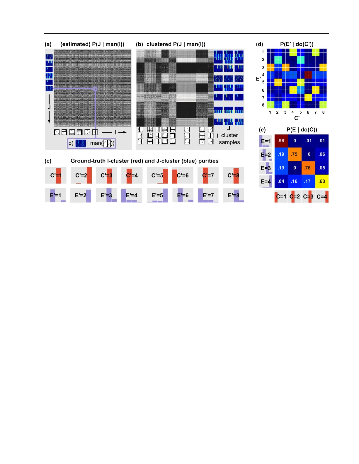
Original Paper
Loading high-quality paper...
Comments & Academic Discussion
Loading comments...
Leave a Comment