Facility Deployment Decisions through Warp Optimizaton of Regressed Gaussian Processes

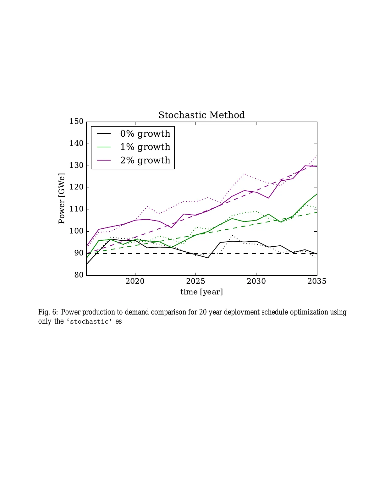
F acility Deplo yment Decisions through W ar p Optimizaton of Regr essed Gaussian Processes Anthony Michael S copatz 1 1 University of South Car olina, Department of Mechanical Engineering, Nuclear Engi neering Pr ogram, Columbia, SC 29201 Send pr oofs to: Anthony M. Scopatz scopatz@cec.sc.edu 541 Main Street, Columbia, SC 29208 Number of Pages: 35 Number of T ables: 0 Number of Figure s: 11 Keyw ords: nuclear fuel c ycle, gaussian process, dynamic time w arping Abstract A method for quickly determinin g deployment schedules that meet a given fuel cycle demand is presented here. This algorithm is fast enough t o perform in si tu within low-fidelity fuel cycle simul ators. It uses Gaussian process regression mod els to predict the produ ction curve as a function of time and the number of deployed facilities. Each of th ese predictions is m easured against the demand curve using the dynamic time w arping distance. The minimum di stance deplo yment schedule is ev aluated in a full fuel cycle simulatio n, whose generated production curve then informs t he model on the next opt imization iteration. The method con verges wit hin five to ten it erations to a distance that is less than one percent of the total deployable production. A representati ve once- through fuel cycle is used to demonstrate the methodology for reactor deployment. I INTR O DUCTION W it h the recent advent of agent-based nucl ear fuel cycle simulato rs, such as Cyclus [1, 2], there comes the possibi lity to make in situ, dynamic facility deployment decision s. This would more fully model real-world fuel cycles where in stitution s (such as utili ty com panies) predict future demand and choose their future deployment schedules appropriately . Howe ver , one of the majo r challenges to mak- ing in situ d eployment decisions is th e speed at which “good eno ugh” decisions can be m ade. This paper proposes three related deployment-specific optimizati on algorithms that can be used for any demand curve and facility type. The demands of a fuel cycle scenario can often be simply stated, e.g. 1% growth in powe r produc- tion [GW e]. Picking a deployment schedule for a certain kind of facility (e.g. reactors) can thus be seen as an optim ization problem of how well the deployment schedule meets the demand. Here, the dynamic time warping (DTW) [3] distance is minimized between the demand curve and the r egression of a Gaussian Process model (GP) [4] of prior sim ulations. This minimization produces a guess for a deployment schedule which is subsequent ly tested using an actual simulator . This process is repeated until an optimal deployment schedule for the gi ven demand is found. Importantly , by using the Gaussian process s urrogates, th e number of simul ation realization s that must be e xecuted as p art of the o ptimization may be reduced to only a handful. Furthermore, it is at least two orders-of-magnitud e faster to test t he mo del than it i s t o run a s ingle low-fidelity fuel cycle s imulation. Because of the relative comput ational cheapness, it is suitable to be used i nside of a fuel cycle simulation. T raditi onal ex situ optimi zers may be able to find more precise sol utions but at a comput ational cost beyond the scope and need of an in s itu use case that is capable of dynamic adjustment. Every iteration of the war p optimi zation o f regressed Gaus sian processes (WORG) method de- scribed here has two phases. The first is an estimation phase where the Gaussian process mo del is built and ev aluated. The second takes the deployment schedule from the estimati on phase and runs it in a fuel cycle simulator . T he results of the sim ulator of t he s -th iteration are then used to inform the model on the ( s + 1 ) -th iteration. Inside of each estimation phase there are three pos sible strate gies for choosing the next deployment schedule. The first is to sample of th e s pace of all possi ble deployment st rategies stochastically and then take the best guess. The second is to search t hrough the inner product of al l choices, pi cking the best option for each deployment para meter . The third strategy is to perform the two previous strategies and determine which one has picked the better guess. Nuclear fuel cyc le demand curve opt imization faces many challenges. Foremost am ong these is that eve n though the demand curve is specified on t he range of the real numbers, the opt imization parameters are fun damentally integral in nature. F or a discrete time simulator , deployments can only be iss ued in multiples of the s ize of the time step [5]. Furthermore, it is not pos sible to d eploy only part of a f acility; the f acility is either deployed or it is not. Whi le it may be poss ible to deploy a facility and only run it at partial capacity , most fuel cycle models do not suppo rt such a feature for keystone facilities. For example, it is un likely that a utility would b uild a ne w reac tor only to run it at 50% power . Thus, deployment is an integer programming problem, as oppos ed to it s easier lin ear programming cousin [6]. As an in teger programmin g problem, the option s pace is combi natorially lar ge. Assumi ng a 50 year deployment schedul e w here no more than 3 facilities are allowe d t o be deployed each time step, there a re more than 10 30 combinations . If e very simulati on took a very gener ous 1 sec, sim ulating each option would still take ≈ 3 × 10 12 times the current age of the universe. Moreover because all of the parameters are integral, there is not a m eaningful formulation of a continuous Jacobian. Deriv ative-free optimizers are required. Method s such as particle swarm [7], pswarm [8], and the simplex method [6] all could work. Howe ver , typi cal im plementations require more e valuations of the objecti ve function (i.e. fuel cycle sim ulations) than are within an in situ budget. Even the usual case of Gaussian process opt imization (s ometimes known as kriging) [9, 10] will still require too many full realizations in order to form an accurate model. WORG, on the other hand, uses the dynamic tim e warping distance as a measure of how two time series diff er . This is because the DTW d istance is more separativ e than the typical L 1 norm. Such addit ional separation driv es the estimation phase to make better choices soon er . This in turn helps the overall algorithm con ver ge on a reasonable d eployment schedule sooner . The stochastic strategy for WORG addit ionally utilizes Gaussian processes to weight t he choice of parameters. This guides the guesses for t he deployment schedules such that fe w er guesses are needed while simultaneou sly not forbid ding any opti on. So while WORG relies on Gauss ian processes, it does so in a way that is distinct from normal kriging. WORG takes advantage of the a priori knowledge that a deployment s chedule is requested to meet a demand curve. This is not a strategy a generic, of f-the-shelf optimizer would be capable of implementing. The structure of the WOR G algorithm is detailed in §II. The dif ferent strategies for selecting a best guess estimate of the deployment schedule are t hen discussed in §III. Performance and resul ts of the method for a sample once-through fuel cycle scenario are presented in §IV. Finally , §V s ummarizes WORG and lists opportunities for future w ork. II THE WORG MET HOD In order to describe the WORG metho d, first it is is useful to define notatio n for demand curves and their parameterizatio n. Call t the time [years] up to some maximal time horizon T (e.g. 50 years) over which tim e the demand curve is kno wn. Then call f ( t ) the d emand curv e in t he nat ural units of the facility type (such as [GW e] for reactors). f ( t ) may b e any function t hat is desi red, including non-differe ntial functions. For example, though, the demand curve for a 1% gro wth rate s tarting at 90 [GW e] has the following form: f ( t ) = 90 × 1 . 01 t (1) Additionall y , call Θ the d eployment schedule for the fa cilities that may be constructed to meet the demand. Θ is a sequence of P parameters, indexed by p , as seen in Equation 2. Θ = { θ 1 , θ 2 , . . . , θ P } (2) Each θ p represents that num ber of facilities to deploy on i ts time step. In simp le cases where there is on ly one type of facility to deploy P == T . Howe ver , when the deployment schedules of multiple facility types are needed to meet the same demand curve, P > T . The us ual example for P > T is for transition scenarios which necessarily require multipl e ki nds of reac tors. Now denote M as the sequence for the minimu m number of facilities deployable for each deploy- ment parameter . Also, call N the s equence of the maximu m number of f acilities depl oyable. The deployment parameters are thus each defined on the range θ p ∈ [ M p , N p ] . Furthermore, because only whole numbers of facilities m ay be deployed θ p ∈ N . It is a lso typical, but not required, f or M = 0 . Zero is also the lower boun d for all po ssible θ p as facilities may not be forcibly retired via the deployment schedule. From here, call g ( t , Θ ) the production as a function of ti me for a give n deployment schedule. This has the same units as the demand curv e. T hus for po wer demand and reactor deployments, g is in units of [GW e]. The optimizati on probl em can now be posed as an attemp t to find a Θ that mini mizes th e diffe rence between f and g . IIA Dynamic T ime W arping The questi on of how to t ake the difference betw een the demand curve and the production curve is an important one. The naïve option is to simpl y take the L 1 norm of the dif ference between these two time ser ies, as seen in Equation 3. Howe ver , si nce the g ( t , Θ ) com puted from a simulation is expensiv e, any operation that can meaningfully exacerbate th e difference between time series helps driv e down t he number of optimization iterations. Dynamic ti me warping is just such a mechanism. It computes a d istance between any two ti me series which com pounds the separation between the two. Addition ally , the time series are not required to be of th e same length , though for opti mization purposes there is n o reason for them n ot to be. DTW giv es a measure of the amount that one time series would need t o be warped to become the ot her t ime series. It is, therefore, a holist ic measure th at operates over all tim es. Dynamic time warping is more fully cove red in [3]. Howev er , an optimizati on-rele vant i ntroduction is gi ven here. For the t ime series f and g , there are three parts to dy namic ti me warping. The first is the distance d , which will be m inimized. The second is a cost matrix C that helps compute d by indicating how far a point on f is from anot her point on g . Thirdly , the warp path u is t he mini mal cost curve through the C matrix from the fist point in ti me to the last . The DTW di stance can thus be interpreted as the t otal cost of tra veling the w arp path. The first step in comput ing a dynamic time warp d istance is to assemble the cost matrix. Say that the demand time s eries f has length A indexed b y a , and the production time series g has lengt h B indexed by b . For th e optim ization problem here, A and B are in practice bot h equal to T . Howe ver , it is useful to ha ve a and b index th e two time series separately . Now denote an A × B matrix ∆ L as the L 1 norm of the dif ference between f and g : ∆ L a , b = | f ( a ) − g ( b , Θ ) | 1 (3) The cost matrix C may now be defined as the A × B sized m atrix which follows the recursion relation s seen in Equation 4. C 1 , 1 = ∆ L 1 , 1 C 1 , b + 1 = ∆ L 1 , b + C 1 , b C a + 1 , 1 = ∆ L a , 1 + C a , 1 C a + 1 , b + 1 = ∆ L a , b + min  C a , b , C a + 1 , b , C a , b + 1  (4) The b oundary condit ions above are the s ame as setting an infinite cost to any a ≤ 0 or b ≤ 0. The cost matrix C has the sam e units as the demand curve. Howe ver , the scale of C is larger than the demand, e xcept for in t he fiducial c ase. This is because the cost matrix compoun ds the minim um v alu e of pre vious entries. Knowing a cost matrix, the warp path can be com puted by trave rsing the matrix backwards from the ( A , B ) corner t o the ( 1 , 1 ) corner . If the lengt h of the warp i s I indexed by i , the warp path i tself can be thoug ht of as a sequence of coordinate points u i . For a g iv en point u i in the warp p ath, th e pre vious point u i − 1 may be found by pi cking the minimum cost point among the lo cations one column over ( a , b − 1 ) , one ro w ov er ( a − 1 , b ) , and one previous di agonal element to ( a − 1 , b − 1 ) . Equation 5 expresses this m athematically . u i − 1 = argmin  C a − 1 , b − 1 , C a − 1 , b , C a , b − 1  (5) The maximum possible length of u is thus max ( I ) = A + B . T he minimum possibl e l ength, though , is min ( I ) = √ A 2 + B 2 . The dynamic tim e warping distance distance d can now be stated as the cost of t he fi nal entry of the warp path normalized by the maximum possible length of the war p path. d ( f , g ) = C A , B A + B (6) Howe ver , because the demand curve and the production curve are often defined on the same t ime grid, d can be further reduced to the following: d ( f , g ) = C T , T 2 T (7) Therefore, d has the same units as the demand curve, producti on curve, and cost matrix. As an example, t ake a 1% growth t hat starts wit h 90 GW e in the year 2016 as the demand curve. Then consid er a production curve that under-produces the demand by 5% for 25 years before switching to over -producin g thi s curve by 5% for the next 25 years. Figure 1 shows the dynamic time warping cost matrix between these two time series as a heat map. 2 0 2 0 2 0 3 0 2 0 4 0 2 0 5 0 2 0 6 0 t i m e [ y e a r] 2 0 2 0 2 0 3 0 2 0 4 0 2 0 5 0 2 0 6 0 t i m e [ y e a r] 0 2 0 0 4 0 0 6 0 0 8 0 0 1 0 0 0 1 2 0 0 1 4 0 0 C os t [ G W e ] Fig. 1: Heat map o f the cost matrix between a 1% growth demand curve and a production curve the under produces by 5% for th e first 25 years and then over produces for the second 25 years. T he warp path u is superimposed as the white curve on top of the cost matrix. Additionall y , the warp path be tween the e xample demand and production curves is presented as the white curve on top of the heat map in Figure 1. Recognize t hat u is monotoni c along both time axes. Furthermore, the precise path of u min imizes the cost m atrix at e very step. Regions of increased cost in the cost matrix can be seen t o repel the warp path. The dis tance d between the demand and production curves her e happens to be 0.756 GW e. Dynamic time warping distance can t herefore be used as an objective f unction to minim ize for any demand and prod uction curves. Ho wev er , using full simulatio ns to fi nd g ( t , Θ ) remains e xpensive, even though DTW itself is com putationally cheap. Th erefore, a mechanism to reduce the overhead from production curve e valuation is needed. IIB Gaussian Pr ocess Regr ession Evaluating the production curve for a specific kind of fac ility using full fuel cycle simul ations is relatively expensiv e, eve n in th e com putationally cheapest case of low-fidelity sim ulations. This is because a fuel cycle realization ty pically comput es many features t hat, though coupled to the production curve, a re not directly the production curve. For example, the mass balance of the fuel c ycle physically bound the electricity productio n. Howe ver , the mass balances are not explicitly taken in to account wh en trying to meet a power demand curve. Alternative ly , surrogate models that predict the production curve directly have m any orders-of- magnitude fewer operations by vi rtue of not com puting i mplicit ph ysical characteristi cs. This i s not to say that the surrogate models are correct. Rather , t hey are simp ly good enough to driv e a demand curve optimization . Surrogate models are used here inform a simulator about where in the parameter space to look next. Tr uth about production curves sho uld still be deriv ed from th e fuel cycle si mulator and not the surrogate model. In t he WORG algorithm, Gaussian processes are used to form the model. Gaussian processes are more fully covered else where [ 4]. Us ing Gaussian process for optim ization has also been previously explored [9], though such studies tend not to in vestigate the integral problems posed by facility deployment. As with dy namic tim e warping, a m inimal but sufficient introducti on to GP regression i s presented for th e purposes of the deployment optim ization. Consider the case of Z simulatio ns indexed by z that eac h hav e a Θ z deployment schedule and g z ( t , Θ z ) production curve. A Gaussi an process of th ese Z simulati ons is set by i ts mean and cov ariance functi ons. The mean function is denoted as µ ( t , Θ ) and is the expectation va lue E of the series of G inputs: G = { g 1 ( t , Θ 1 ) , g 2 ( t , Θ 2 ) , . . . , g Z ( t , Θ Z ) } (8) The covar iance function is denoted k ( t , Θ , t ′ , Θ ′ ) and is the e xpected value of the i nput to the mean. The mean and cov ariance can be e xpressed as in Equations 9 & 10 respecti vely . µ ( t , Θ ) = E G (9) k ( t , Θ , t ′ , Θ ′ ) = E  ( g z ( t , Θ ) − µ ( t , Θ ))( g z ( t ′ , Θ ′ ) − µ ( t ′ , Θ ′ ))  (10) Note that in th e above, the Gaussi an p rocess is itself P + 1 di mensional, sin ce the m eans and co va riance are a function of both the deployment schedule ( P ) and time ( + 1). The Gaussian process GP approximates the produ ction curve given Z s imulations . All ow ∗ to indi- cate that the a quantity comes from the model as opposed to coming from th e results of the simulator . A model production curve can then be written using either functi onal or op erator notation, as appropriate: g ∗ ( t , Θ ) ≈ GP  µ ( t , Θ ) , k ( t , Θ , t ′ , Θ ′ )  ≡ GP G (11) In machine learning terminology , G serves as the train ing set for the GP model. Now , when p erforming a regression on Gaussian processes, the nominal functi onal form for t he cov ariance must be given. Such a functional form i s also k nown as the the kernel functi on. The kernel contains the hyperparameters that are solved for to obtai ned a b est-fit Gaussian process. The hyp erpa- rameters themsel ves ar e defined based on the definitio n of the kernel function. Hyp erparameter values are found via a regression of the m aximal l ikelihood of the productio n curve. Any functional form could potenti ally serve as a kernel functi on. Howe ver , a generally useful form is t he is the exponen- tial s quared. Thi s kernel can be seen in Equati on 12 with h yperparameters ℓ and σ 2 for a vector of parameters r : k ( r , r ′ ) = σ 2 exp  − 1 2 ℓ ( r − r ′ ) 2  (12) Howe ver , other kernels such as the Matérn 3 / 2 kernel and Matérn 5 / 2 kernel [11] were observed to be more rob ust for the WORG method. These can be seen in Equations 13 and 14 respectiv ely . k ( r , r ′ ) = σ 2 1 + √ 3 ℓ | r − r ′ | ! exp − √ 3 ℓ | r − r ′ | ! (13) k ( r , r ′ ) = σ 2 1 + √ 5 ℓ | r − r ′ | + 5 3 ℓ 2 | r − r ′ | 2 ! exp − √ 5 ℓ | r − r ′ | ! (14) From here, say that K is a covariance matrix such that th e elem ent at th e r -th row and r ′ -th colum n is giv en by whichev er kernel is chosen from Equati ons 12-14. Then the log li kelihood log q of obtaini ng the training set productio n curves G for a giv en time grid t and d eployment schedule is as seen in Equation 15. log q ( G | t , Θ ) = − 1 2 G ⊤  K + τ 2 I  − 1 G − 1 2 log   K + τ 2 I   − Z T P 2 log 2 π (15) Here, τ is the uncertainty in the produ ction curves coming from t he simulatio ns themselves. As mo st simulators do not report such uncertainties, τ may be set to floating poi nt precision. I is the usual identity matri x. The hy perparameters ℓ and σ 2 are then adjust ed via standard real-valued op timiza- tion methods such that Equat ion 15 i s as clo se t o zero as possible. This regression of the Gaussian process its elf yields the most likely m odel of the production curve k nowing o nly a l imited num ber of simulatio ns. Howe ver , the purpose of such a Gaussi an process regression is to ev aluate the p roduction curve at points in time and for depl oyment schedules that ha ve not been simulated. T ake a time grid t ∗ and a hypothetical deployment schedule Θ ∗ . Now call the covariance v ector between the training set and the model e valuation k ∗ = k ( t ∗ , Θ ∗ ) . The production curve predicted by this Gaussian process is then given by the following: g ∗ ( t ∗ , Θ ∗ ) = k ⊤ ∗  K + τ 2 I  − 1 G (16) Equations 9-16 are deri ved and discussed ful ly in [4]. Implementing the above Gaussian process mathematics for the sp ecific case of the WORG alg orithm is not needed. Free and open source Gaussi an proce ss modeling software libraries already e xist and are applicable to th e regression problem here. Scikit-learn v0.17 [12] and George v0.2.1 [13] implement such a method and have a Python int erfac e. George is specialized around Ga ussian processes, and thus is preferred for WORG o ver scikit-learn, which is a gener al purpose machine learning library . As an example, consider a G aussian process between two power producti on curves simi lar t o the example used in §IIA. The first is a nomi nal 1% gro wth in GW e for 50 yea rs starti ng at 90 GW e in 2016. The second curve under-produces the first curve by 10 % for the first 25 years and over -produces by 10% for the last 25 years. Add itionally , assume that there is a 10% error on t he training set data. This will produce a model of the mean and cov ariance t hat splits the difference bet ween these two curves. Thi s example may be seen graphically in Figure 2 . The simple example abov e does not take advantage of an important feature o f Gaussian processes. Namely , it is no t limited to t wo producti on curves in the traini ng set. As many as desirable m ay be used. This wi ll allow the W ORG alg orithm t o dynami cally adjust the number of Z si mulations which are used to predict the next deplo yment schedule. WORG is thus capable of ef fortlessly expanding Z when new a nd us eful simulati ons yield valuable production curves. Howe ver , it also enables Z to contract to discard production curves t hat would dri ve the deployment schedule away from an op timum. Now that the Gaussian process regression and dynamic t ime warping too ls have been added to the toolbox, the architecture of the WORG algorithm can itself be described. 2 0 2 0 2 0 3 0 2 0 4 0 2 0 5 0 2 0 6 0 t i m e [ y e a r] 0 2 0 4 0 6 0 8 0 1 0 0 1 2 0 1 4 0 1 6 0 P owe r P rod u c t i o n [ G W e ] t r a i n g d a t a m o d e l Fig. 2: The Gaus sian process m odel of a 1% growth curv e along wi th the an initial 10% under produc- tion f ollowed by a 10% under producti on. Th e m odel is represented by the bl ack li ne that runs between the red training points. T wo standard de viations form the model are displayed as the gray re gion. IIC WORG Algorithm The WORG algorithm has two fundamental phases o n each iteratio n: estimation and sim ulation. These are preceded by an initi alization before the opti mization loop. Additionally , each iteration de- cides which inform ation from th e previous simu lations is worth keeping for the next esti mation. Fur - thermore, the method of estimati ng deployment schedules may be altered each iteration. Listing 1 shows the WORG algorithm as Python p seudo-code. A detailed walkthrough explanation of th is code will now be presented. Begin by initi alizing three empty sequences ~ Θ , G , and D . Each element of these series represents deployment schedule Θ , a production curve g ( t , Θ ) , and a dynami c time warping history between the demand and production curves d ( f , g ) . Importantly , ~ Θ , G , and D only contain values for the rele va nt optimizatio n window Z . For example, root finding algorithm s such as Newton’ s method and the bisec- tion method ha ve a length-2 wi ndow since they use the ( z − 1 ) th point and the z th point to com pute the ( z + 1 ) th guess. Since a Gaussi an process model i s formed, any or all of t he s iterations may be used. Howe ver , restricting the opt imization wi ndow to be either two or three depending on th e circums tances balances the need to keep t he points wit h the lowest d values while pushing the model far from known regions with higher dist ances. Essentially , WORG tries to ha ve D contain o ne high-value d and one o r two lo w v alued d at all iterations. Such a tactic helps form a m eaningfully di verse GP m odel. T o thi s end, ~ Θ , G , and D are initialized with two bounding cases. The first is to set the deployment schedule equal to the lo wer bound of the number of depl oyments M . Recall that this is usually 0 e very- where, unless a mini mum number o f facilities must be deployed at a specific point in time. Running a simulatio n with M will then yield a production curve g ( f , g ) and t he DTW distance to this curve. Not e that just because the n o facilities are deployed, the production curve need not be zero due to the initial conditions of the simulation. Existing initial facilities will continue to be productiv e. Similarly , another simulation may be exe cuted for t he maxim um possible deployment schedule N . This w ill als o provide inform ation on the production over time and t he distance t o the demand curve. M and N form the first two simulation s, and therefore t he loop v ariable s is set to two. Listing 1: WORG Algorithm in Python Pseudo-code T h e t a s , G , D = [ ] , [ ] , [ ] # i n i t i a l i z e h i s t o r y # r u n l o w e r b o u n d s i m u l a t i o n g , d = r u n _ s i m ( M , f ) T h e t a s . a p p e n d ( M ) G . a p p e n d ( g ) D . a p p e n d ( d ) # r u n u p p e r b o u n d s i m u l a t i o n g , d = r u n _ s i m ( N , f ) T h e t a s . a p p e n d ( N ) G . a p p e n d ( g ) D . a p p e n d ( d ) s = 2 w h i l e M A X _ D < D [ - 1 ] a n d s < S : # s e t e s t i m a t i o n m e t h o d m e t h o d = i n i t i a l _ m e t h o d i f m e t h o d = = ' a l l ' a n d ( s % 4 < 2 ) : m e t h o d = ' s t o c h a s t i c ' # e s t i m a t e d e p l o y m e n t s c h e d u l e a n d r u n s i m u l a t i o n T h e t a = e s t i m a t e ( T h e t a s , G , D , f , m e t h o d ) g , d = r u n _ s i m ( T h e t a , f ) T h e t a s . a p p e n d ( T h e t a ) G . a p p e n d ( g ) D . a p p e n d ( d ) # t a k e o n l y t h e m o s t i m p o r t a n t a n d m o s t r e c e n t s c h e d u l e s i d x = a r g s o r t ( D ) [ : 2 ] i f D [ - 1 ] = = m a x ( D ) : i d x . a p p e n d ( - 1 ) T h e t a s = [ T h e t a s [ i ] f o r i i n i d x ] G = [ G [ i ] f o r i i n i d x ] D = [ D [ i ] f o r i i n i d x ] s = ( s + 1 ) The opti mization loop may now be entered. This loop has two conditions . The first is that the n ext iteration occurs only if the last distance is greater than a threshold value MAX_D. T he second is that the loop v ariable s must be less than the maximum number of iteration S . The first s tep in each iteration is to choose the esti mation method. The three m echanisms will be discus sed in detail in § III. For the purposes of the op timization loop, they may be represented by the ‘stochastic’ , ‘inner-prod’ , and ‘all’ flags. The stochastic method chooses many random deployment schedules to test. Al ternativ ely , an inner product search of t he space defined by M and N may be performed. Lastly , the ‘all’ flag performs both of the pre vious estimates and takes the o ne with lowest computed distance. Howe ver , ‘all’ can sometimes declare the i nner product search the winner for all s . This can i tself be prob lematic since thi s estimation meth od has the tendency to form deterministic loops when close to an opt imum. This behavior is not unlike sim ilar loops formed with floating point approximations to Newton’ s method. T o prev ent thi s when using ‘all’ , WORG forces the stochastic method for two consecuti ve it erations out of e very four . A best-guess esti mate for a deployment schedule Θ may finally be made. This takes the previous deployment s chedules ~ Θ and prod uction curves G and form s a Gaussi an process model. Potent ial values for Θ are explored according to t he selected estim ation m ethod. The Θ that produces the min imum dynamic time warping distance between the demand curv e and the model d ( f , g ∗ ) is then returned. The Θ estim ate is then supplied t o the the simu lator itself and a sim ulation is exe cuted. T he details of this procedure are, of course, sim ulator specific. Howe ver , the simu lation combined wit h any post- processing needed should return an aggregate production curv e g s ( t , Θ ) . This is then com pared to demand curve via d ( f , g s ) . After the simul ation, Θ , g s ( t , Θ ) , and d ( f , g s ) are appended to the ~ Θ , G , and D sequences. No te that t he p roduction curve and DTW distance from the simulator are appended, not the production curve and di stance from the model estimate. Concluding the optimi zation loop, ~ Θ , G , D , and s are updated. T his begins by finding and keeping the two elements with the lowest distances betw een the demand and production curves. Howe ver , if the most recent simulatio n yielded the largest distance, th is is also kept for the next iteration. Ke eping the lar gest distance serves t o deter exploration in this di rection on the next i teration. Th us a sequence of two or three indices is chos en. These indices are applied to redefine ~ Θ , G , and D . Lastly , s is incremented by one and the next it eration begins. The WORG algorithm presented here shows th e overall structure of th e optimization. Howe ver , equally important and not covered in this section is how the estimation phase chooses Θ . Th e methods that WORG may use ar e presented in the following section and completes the methodology . III SELECT ING DEPLO YMENT SCHEDULE ESTIMA TES There are three method s for choosing a ne w deployment schedule Θ to a ttempt to run in a simulator . The first is st ochastic with weighted probabilities for the θ p . The second does a deterministic sweep iterativ ely over all options , minimi zing t he d ynamic time warping di stance at each p oint i n ti me for each deployment parameter . The last com bines these two and choose the one with the minim um distance to the demand curve. All of these rely on a Gaussian process model of the production curve. This is because constructing and e v aluating GP model g ∗ is significantly f aster than performing e ven a low-fidelity simulation. As a demonstrative example, say each ev aluation of d ( f , g ∗ ) tak es a tenth of a second (whi ch is excessi vely long) and d ( f , g s ) for a low fidelity s imulation takes ten seconds (which is reasonable), th e model e valuation is still o ne hu ndred times faster . Furthermore, the cos t of constructing the GP m odel can is amortized ove r the number of guesses that are made. Howe ver , the choice of which θ p to pick is extremely important as they drive the optimi zation. In a vanilla stochastic algorithm, each θ p would b e selected as a univ ariate integer on t he range [ M p , N p ] . Howe ver , this ignores the distance inform ation D that is known about the traini ng set which is used to create the Gauss ian process. More intelligent guesses for θ p focus th e model e valuations t o mo re promising re gions of the option space. This in turn helps reduce the overall number of expensive simulatio ns needed to find a ‘goo d enough’ deployment schedule. The three WORG Θ selection methods are described in order in the follo wing subsections. IIIA Stochastic Estimation The stochastic method works by random ly choos ing Γ deployment schedules and ev aluating g ∗ ( t , Θ γ ) for each guess γ . Th e Θ γ which has the min imum distance d γ is taken as the best -guess deployment schedule. The number of guesses may be a s large or as s mall as desi red. Howe ver , a re asonable nu mber to pick spans the option space. This is simply i s the L 1 norm of the difference of t he inclusive bounds. Namely , set Γ as in Equation 17 for a minimum number of for stochastic guesses. Γ = P ∑ p ( N p − M p + 1 ) (17) Each θ p has N p − M p + 1 options. Thus a reasonable choice for Γ is the sum of the number of indepen- dent options. Still, each option for θ p should not be equally likely . For example, if the demand curve is relati vely low , th e number of deployed f acilities is unlikely to be relati vely high. For this reason, the choice of θ p should be weighted. Furthermore, note that each θ p is po tentially weight ed differe ntly as t hey are all independent parameters. Denote n ∈ [ M p , N p ] such that the n-th weight for th e p-th parameter is called w n , p . T o choose weights, first observe th at t he distances D can be said to be in ve rsely proportional to how li kely each deployment schedule in ~ Θ should be. A one-dimensional Gaussian process can thus be constructed to mod el in verse distances giv en the v alues of the deployment parameter for ea ch schedule, namely ~ θ p . Call this model d − 1 ∗ as seen in Equation 18. d − 1 ∗ ( θ p ) = G P  µ ( ~ θ p ) , k ( ~ θ p , ~ θ p ′ )  ≡ GP  D − 1  (18) The constructi on, regression of hyperparameters, and ev aluation of this m odel follows analogously t o the production curve modeling presented in §IIB. The weights for θ p are then the normalized e valuation of the in verse distance model for all m and n defined on the p-th range. Symbolically , w n , p = d − 1 ∗ ( n ) ∑ N p m = M p d − 1 ∗ ( m ) (19) Equation 19 works very well as long as a valid m odel can be establish ed. Howe ver , this is sometim es not the case when the θ p are de generate, the distances are too close together , the distances a re too clos e to zero, or other stability issues arise. In cases where a valid model may not be formed for d − 1 ∗ ( θ p ) , a Pois son distribution may be used instead. T ake the m ean of t he Poisson distribution λ to be t he value of θ p where the distance is m ini- mized. λ p = θ p | argmin ( D ) (20) Hence, the Poisson probability distribution for the n -t h weight of the p -th deployment parameter is, Poisson ( n ) = ( λ p ) n n ! e − λ p (21) Now , because n is boun ded, it i s im portant to renormalize Equati on 21 when cons tructing stochastic weights. w n , p = ( λ p ) n n ! e − λ p ∑ N p m = M p ( λ p ) m m ! e − λ p = ( λ p ) n n ! ∑ N p m = M p ( λ p ) m m ! (22) Poisson-based weights c ould be used e xclusively , foregoing th e in verse distance Gaussian process mod- els compl etely . Howe ver , a Poisson-only method takes in to account less inform ation about the dem and- to-production curve distances. It was therefore observed to conv er ge more slowly on an opti mum than using Poisson weigh ts as a backup. Since the total number of simulation s is aiming to be m inimized for in situ use, the WORG method uses Poisson weights as a fa llback only . After weights are computed for all P deployment parameters, a set of Γ deployment schedules may be stochastically chosen. The Gaussian process for each g ∗ ( t , Θ γ ) is then ev aluated and t he dynamic time warping dis tance to the demand curve is comput ed. The deployment schedule wi th th e minim um distance is then selected and returned. IIIB Inner Pr oduct Estimation As an alternative to the stochastic met hod dem onstrated in §IIIA, a best-guess for Θ can also be built up iterativ ely over all times. The method here uses t he same production curve Gaussian process g ∗ to predict production lev els and measure the distance to the demand curve. Howe ver , this m ethod minimizes the dist ance at time t and then uses this to inform the minimization of t + 1. Starting a t t = 1 and moving t hrough the whole time grid to t = T , a complete deployment schedu le is generated. The following description is for the simpl ified case when P = = T . Howe ver , this method is easily extended to the case where P > T , such as for multiple rea ctor types. When P > T , group θ p that occur on the same time step tog ether and take the ou ter product of their options prior t o steppi ng th rough time. For t his method, define the time s ub-grid t p as the sequence of all times less than or equal to th e time when parameter p occurs, t ( p ) . t p = { t | t ≤ t ( p ) } (23) Now define the deployment schedule Θ t up to time t through the following recursion r elations: θ 1 = n | min [ d ( f , g ∗ ( 1 , n ))] ∀ n ∈ [ M 1 , N 1 ] Θ 1 = { θ 1 } θ p = n | min  d ( f , g ∗ ( t p , Θ t − 1 , n ))  ∀ n ∈ [ M p , N p ] Θ t = n Θ t − 1 1 , . . . , Θ t − 1 p − 1 , θ p o (24) Equation 24 h as t he ef fect of choosing the the number of facilities to deploy at each t ime step that minimizes the distance fun ction. T he c urrent tim e step uses the previous deployment schedule and only searches the option space o f the its own deployment p arameter θ p . Once Θ T is reached, it is selected as the deployment schedule Θ . The inner product m ethod here requires the same number o f m odel e valuations of g ∗ as were selected for the def ault value of Γ in Equation 17 for stochastic estimation. IIIC All of the Abo ve Estimation This method is simply to run both the stochastic method and the inner product metho d and determine which has t he l ower d ( f , g ∗ ) for the deployment schedules the y produce. This m ethod cont ains both the adva ntages and di sadvantages of i ts cons tituents. Additional ly , it has the disadvantage of bei ng more computationall y expensive t han the other methods individually . The adv antage from the st ochastic method is that the entire space is potentially sea rched. There are no forbid den regions. This is important s ince there may be other optim a far away from the current ~ Θ that produ ce lower di stances. Searching globally prevents the stochastic meth od from becoming stuck locally . Howe ver , the sto chastic metho d may take m any iteration s to make minor improvements on a Θ which is already close to a best-guess. It is, after all, searching globally for something better . On the ot her hand, the inner product method is desig ned to search around the part of the Gaussian process model which already produces go od results. It is meant to make minor adj ustments as i t goes. Unfortunately , this means the inner product method can m ore easily get stuck in a cycle where i t pro- duces the same ser ies of deployment schedules o ver and over again. It has no mechanism on its o wn to break out of such cycles. W it h the all-of-the-above option , the job of balancing the relati ve merits of the st ochastic and inner product m ethods is left to the optimi zation loop itself. This can b e s een in §IIC. If the ‘all’ flag is set as the esti mation method, it is only ex ecuted as the ‘all’ flag two of ev ery four iteratio ns. Other strategies for determining how and when each of th e three methods are us ed could be designed. Ho we ver , any more complex strategy should be able to sho w that it meaningfull y re duces the number of opt imization loop iterations required. At this point, t he ent ire WORG method has been described. A demonstration of how it performs for a representativ e fuel cycle is presented in the next section. IV RESUL TS & PERFORMANCE T o demonstrate the th ree variant WORG methods, a n unconstrained on ce-through fuel cycle is mod- eled with the Cyclus simulator [1]. In such a scenario, uranium mini ng, enrichment, fuel fabrication, and storage all ha ve ef fecti vely infinit e capacities. The only meaningful constrain ts on the sy stem are how many light-water reactors (L WR) are b uilt. The base simulati on begins with 100 reactors in 2016 that each produce 1 GW e, have an 18 month batch lengt h with a one m onth reload time. The initial fleet of L WRs retires ev enly over th e 40 years from 2016 t o 2056. All new reactors hav e 60 year l ife tim es. The simulatio n its elf follows 20 years from 2016 to 2035. This is on th e higher end of in situ time hori zons expected, which presumably will be in the neighborhood of 1, 5, 10, or 20 years. The stud y here compares how WORG performs for 0% (steady st ate), 1%, and 2 % growth curves from an initi al 90 GW e target. These are examined using the three estimati on metho ds variants de- scribed in the pre vious section. Calling ρ the growth rate as a fraction, the demand curve is thus, f ( t ) = 9 0 ( 1 + ρ ) t (25) Moreover , t he upper bound for the number of deployable fac ilities at each tim e is set to be t he ceili ng of ten times th e total gro wth. That is, assuming ten fac ilities at most could be deplo yed in the first year , increase the upper bound along with the gro wth rate. This yields the following e xpression for N . N ( t ) =  10 ( 1 + ρ ) t  (26) The lower bou nd for the number of deployed reactors is taken to be t he zero v ector , M = 0 . A m aximum of twenty si mulations are al lowed, or S = 20. Thi s is because an in situ method cannot af ford many optimizatio n iterations . The random seed for all optimization s was 424242. Note that because of t he i ntegral nature of facility deployment, exactly m atching a continu ous de- mand curve is not possibl e in general. Slight over - and under -prediction are expected for mos t points in time. Furthermore, it is unlikely th at the init ial facilities wi ll match the demand curve themselves. If the initial facilities do no m eet the demand on their own, then the optimized deployment schedule is capable m aking up the dif ference. Howe ver if the in itial facilities produce more than the demand curve, the the optimizer is only capable o f deploying zero fac ilities at these t imes. The WORG method does not help make radical adju stments to accommodate p roblems with the ini tial conditio ns, such as when 50 GW e are demanded b ut 100 GW e are already being produced. First e xamine Figures 3 - 5 which show the optimized deployment schedule for the three estimation methods. The figures represent the 0%, 1% and 2% growth curves respectiv ely . Figures 3 & 4 show that the ‘stochast ic’ method has the highest number of facilities deployed at any sin gle time. In the 2% case, the ‘all’ method predicts the largest number of f acilities deployed. 2 0 1 5 2 0 2 0 2 0 2 5 2 0 3 0 2 0 3 5 t i m e [ y e a r] 0 2 4 6 8 1 0 1 2 Nu m b e r o f D e p l o ye d L W R s , Θ 0 % G r o w t h s t o c h a s t i c i n n e r - p r o d a l l Fig. 3: Opti mized deployment schedule Θ for a 0% growth (st eady state) demand curve. The number of deployed facilities sho wn are for the ‘stochastic’ (black), ‘inner -prod’ (green), and ‘all’ (purple) estimation methods. 2 0 1 5 2 0 2 0 2 0 2 5 2 0 3 0 2 0 3 5 t i m e [ y e a r] 0 2 4 6 8 1 0 1 2 Nu m b e r o f D e p l o y e d L W R s , Θ 1 % G r o w t h s t o c h a s t i c i n n e r - p r o d a l l Fig. 4: Opti mized deployment schedul e Θ for a 1% growth demand curve. The number of deployed facilities shown are for the ‘stocha stic’ (black), ‘inner-prod’ (green), and ‘a ll’ (purple) estima- tion methods. 2 0 1 5 2 0 2 0 2 0 2 5 2 0 3 0 2 0 3 5 t i m e [ y e a r] 0 2 4 6 8 1 0 1 2 Nu m b e r o f D e p l o y e d L W R s , Θ 2 % G r o w t h s t o c h a s t i c i n n e r - p r o d a l l Fig. 5: Opti mized deployment schedul e Θ for a 2% growth demand curve. The number of deployed facilities shown are for the ‘stocha stic’ (black), ‘inner-prod’ (green), and ‘a ll’ (purple) estima- tion methods. More important than the depl oyment schedules themselves, howe ver , are the production c urves th at they elici t. Figures 6 - 8 display the po wer produ ction for the best-guess deployment schedule G 1 (solid lines), production for the second b est schedule G 2 (dotted lines), and d emand curves (dashed lines) for 0%, 1%, and 2% gro wth. The figures show e ach estimation mechanism separately . 2 0 2 0 2 0 2 5 2 0 3 0 2 0 3 5 t i m e [ y e a r] 8 0 9 0 1 0 0 1 1 0 1 2 0 1 3 0 1 4 0 1 5 0 P o w e r [ G W e ] S t o c h a s t i c M e t h o d 0 % g r o w t h 1 % g r o w t h 2 % g r o w t h Fig. 6: Po wer productio n to demand com parison for 20 year deployment schedule op timization using only the ‘stoc hastic’ estimation m ethod. 0%, 1%, and 2% growth rates starti ng at 90 GW e are shown. Solid lines represent th e best guess deployment schedule. Dott ed lines are represent the second best guess deployment schedule. Dashed l ines represent the demand curve that is targeted. As seen in Figure 6, the ‘stoch astic’ onl y estim ations follow the trend line of the growth curve . Howe ver , only for a fe w re gions such as for 2% growth between 2025 - 2030, does the production very closely match th e the demand. The second best guess for the deployment schedule shows a relatively lar ge degree of eccentricity . T his i ndicates th at G 2 at the end of the optimization i s there to show the Gaussian process model re gions in the Θ option space that do not work. Alternative ly the inner prod uct search esti mation can be seen in Figure 7. This method does a 2 0 2 0 2 0 2 5 2 0 3 0 2 0 3 5 t i m e [ y e a r] 8 0 9 0 1 0 0 1 1 0 1 2 0 1 3 0 1 4 0 1 5 0 P o we r [ G W e ] I n n e r P r o d u c t M e t h o d 0 % g r o w t h 1 % g r o w t h 2 % g r o w t h Fig. 7: Po wer productio n to demand com parison for 20 year deployment schedule op timization using only the ‘inne r-prod’ estimation m ethod. 0%, 1%, and 2% growth rates starti ng at 90 GW e are shown. Solid lines represent th e best guess deployment schedule. Dott ed lines are represent the second best guess deployment schedule. Dashed l ines represent the demand curve that is targeted. reasonable job of predicting a st eady state scenario at later ti mes. Ho wev er , the 1% and 2% curves are largely un der -predicted. For th e 2% case, this is s o severe as t o be considered wholly wrong. This situation aris es because the ‘inner-prod’ method can enter in to determi nistic traps where the same cycle o f deployment schedules is predicted forever . If such a t rap is fallen into when th e productio n curve is far from an optimu m, the inner product method does not yield a suffic iently close guess of the deployment schedule. Howe ver , combining the stochastic and inner product estimati on methods lim its the weakness of each m ethod. Figure 8 shows the production and dem and inform ation for the ‘all’ estim ation flag. By i nspection, this meth od produces production curves that match the demand much more closely . This is especially true for later times. Over -prediction discrepancies for early times come from the fact the initially deployed facilities (100 L WRs wi th 18 month cycles) does not precisely m atch an initial 90 2 0 2 0 2 0 2 5 2 0 3 0 2 0 3 5 t i m e [ y e a r] 8 0 9 0 1 0 0 1 1 0 1 2 0 1 3 0 1 4 0 1 5 0 P o we r [ G W e ] A l l M e t h o d 0 % g r o w t h 1 % g r o w t h 2 % g r o w t h Fig. 8: Po wer productio n to demand com parison for 20 year deployment schedule op timization using the ‘all’ estimati on method that s elects the best of b oth ‘stochastic’ and ‘inner-pro d’ estima- tions. 0%, 1%, and 2% growth rates starting at 90 GW e are shown. Solid lines represent th e best guess deployment schedule. Dotted li nes are represent the second best guess d eployment schedule. Dashed lines represent the demand curve th at is tar geted. GW e tar get. The problem was specified this w ay in order to show that reasonable deployments are still selected e ven in slightly unreasonable s ituations. Still, the main purpose of the WORG algorithm is to con ver ge as qu ickly as po ssible to a rea sonable best-guess Θ . The li miting factor i s the number of predi ctiv e si mulations which must be run. WORG will always ex ecute at least three full simulati ons: t he lower bound, the upper bound, and one iteration of t he optimization lo op. A reasonabl e limit on the total number of simulations S i s 2 0. For an in situ calculator , it is unl ikely to want to compu te more than this num ber o f sub-simul ations to p redict the deployment schedule for the n ext 1, 5 , 10, or 20 years. H owe ver , it may be possibl e to limit S to significantly belo w 20 as well. Figures 9 - 11 demonstrate a con ve rgence study for t he three differe nt growth rates as a functi on 5 1 0 1 5 2 0 S i m u l a t i o n s 1 0 - 1 1 0 0 1 0 1 1 0 2 M i n i m u m D i s t a nc e , d ( f , g s ) [ G W e ] 0 % G r o w t h s t o c h a s t i c i n n e r - p r o d a l l Fig. 9: Con ver gence of 0% growth rate solution for the distance between the demand and produ ction curves d ( f , g ) as a function of the number of sim ulations. The three estimation methods are shown. Additionall y , the S , I , and A marker represent wheth er the ‘stochastic ’ , ‘inner-pr od’ , or ‘all’ method was selected as the best fit. For 2 < s , the ‘all’ wil l select either S or I . of the num ber of sim ulations s . These three figures demonstrate important properties of t he WORG method. The first is that the ‘all’ estimation method here consistentl y has t he lowest min imum dynamic time warping dist ance, and t hus the best guess for the deployment schedul e Θ . Further- more, the ‘all’ curves in these figures sh ow th at the best est imation met hod consis tently switches between the in ner product search and stochastic search. These i mply that t ogether the ‘stochastic’ and ‘inner-prod’ methods con ver ge more qui ckly that th e sum of their parts. This is particularly visible in the 0% growth rate case seen i n Figure 9. Additionall y , These con vergence plots show that the majorit y of the Θ selection gains are made by s = 1 0. Simulations past ten may sho w differential improv ement f or the ‘all’ method . Ho wev er , they do not tend to generate any measurable improvement for ‘stocha stic’ or ‘inner-pr od’ selection mechanisms. Furthermo re, most of the gains for the ‘all’ meth od are realized by simu lation fi ve or 5 1 0 1 5 2 0 S i m u l a t i o n s 1 0 - 1 1 0 0 1 0 1 1 0 2 M i n i m u m D i s t a nc e , d ( f , g s ) [ G W e ] 1 % G r o w t h s t o c h a s t i c i n n e r - p r o d a l l Fig. 10: Con ver gence of 1% growth rate sol ution for t he distance between the demand and production curves d ( f , g ) as a function of the number of sim ulations. The three estimation methods are shown. Additionall y , the S , I , and A marker represent wheth er the ‘stochastic ’ , ‘inner-pr od’ , or ‘all’ method was selected as the best fit. For 2 < s , the ‘all’ wil l select either S or I . six. Thus a reduction by a factor of two to four i n the nu mber of sim ulations is av ailable. This equates directly to a like reduction in computational cost. Moreover , Figures 9 - 11 also sho w th e t endency of the ‘inner-prod’ method to become determin- istically st uck when used on its own. In all three cases the ‘inner-prod’ m ethod reso lves to a constant by si mulation fiv e or ten. In the 1% case, this solutio n happens to be quite close t o the soluti on predicted by the ‘all’ m ethod. In the 0% case, this const ant is meaningfully di stinct, but is st ill more akin to the ‘stochast ic’ solutio n than the ‘all’ solutio n. In the 2% case, the con verged ‘inner-prod’ result has little to do wi th the ‘all’ prediction. Thus it i s not recommended to use ‘inner-prod’ on it s own. While it may succeed, it is too risky because it may cease improving at the wrong place. The ‘stochastic’ estimation method is also pron e to s imilar cyclic beha vior . Ho we ver , in the ‘inner-pr od’ method, is the second best guess G 2 is also in a constant predicti on cycle along with G 1 . 5 1 0 1 5 2 0 S i m u l a t i o n s 1 0 - 1 1 0 0 1 0 1 1 0 2 M i n i m u m D i s t a nc e , d ( f , g s ) [ G W e ] 2 % G r o w t h s t o c h a s t i c i n n e r - p r o d a l l Fig. 11: Con ver gence of 2% growth rate sol ution for t he distance between the demand and production curves d ( f , g ) as a function of the number of sim ulations. The three estimation methods are shown. Additionall y , the S , I , and A marker represent wheth er the ‘stochastic ’ , ‘inner-pr od’ , or ‘all’ method was selected as the best fit. For 2 < s , the ‘all’ wil l select either S or I . W it h the stochastic s earch, the second best guess has more freedom to roam the opti on space, creating potentially diffe rent Gaussian process models with each iteration s . Eventually , giv en enough guesses and enough iterations, t he stochastic mo del will break out of a local optimum to perhaps find a better global optimum elsewhere. F or th e in situ use case, though, eventual sol ution is not fast enough. The inner product search spans regions that t he stochastic weighting labeled as unlikely . This assi st is what enables the ‘all’ meth od to con ver ge faster than the s tochastic method on its own. That said, if the in situ use case is not rele v ant, the stochastic method on its own could be used without an y algorithmic qualms. V CONCLUSIONS & FUTURE WORK The WORG method provides a deployment schedule optimizer that con verges both closely enough and fast enough to be used ins ide of a nuclear fuel cycle sim ulator . The algorithm can consistently obtain tolerance s of half-a-percent to a percent (1 GW e distances for ov er 20 0 GW e deployable) for the once-through fuel cycle featured here within only fi ve to ten simulations. Such opt imization probl ems are made m ore chall enging due to the integral nature of facility deployment and that any demand curve may be requested. WORG works by s etting up a Gaussian process to m odel the production as a function of tim e and the deployment schedule. This model m ay then be ev aluated orders of m agnitude faster than running a ful l simulation, enabling t he search over m any potential deployment schedul es. The quality of these possible schedules is ev aluated based o n the dyn amic time warping distance to t he demand curve. The lowest dist ance curve is th en ev aluated i n a full fuel cycle si mulation. The prod uction curve that i s computed by th e simul ator in turn goes on to u pdate the Gauss ian process mo del and the cycle repeats until the limiting conditions are met. Howe ver , choosin g the deployment schedules to estimate with the Gauss ian process may be per- formed in a num ber of ways. A blind approach would sim ply b e t o choose s uch schedules randomly from a univariate. Howe ver , the WORG m ethod has m ore i nformation a va ilable to it that helps drive down th e number of loop iterations. The first method discus sed remains stochastic but us es the in verse DTW dist ances of the GP model to weight the deployment options , falling back to a Poisson di stri- bution as necessary . Th is second m ethod m inimizes the model dis tance for each point i n time from start to end, iterative ly building up a soluti on. Finally , another est imation st rategy tries both previous options and chooses th e best result, forcing the stochast ic method two of e very four iterations t o av oid deterministic loops. It is this last all-of-the-above method th at is seen to con ver ge the fastest and to the lowest distance in most cases. It is important to note that the WORG algorit hm i s appli cable t o any demand curve type and fuel cycle facility type. It is not restricted t o reactors and power . E nrichment and separative work units, reprocessing and separ ations capacity , and deep geologic repositories and their space could be deployed via the WORG m ethod for any applicable demand curve. Reactors were chosen for study here as the representativ e keystone example. The ne xt major step for this work is to actually employ th e WORG method in a fuel c ycle si mulator . Howe ver , to the best knowledge of th e author , no existing simulato r is capable of spawning forks of itself during run tim e, rejoining the processes, and ev aluating the results of the child sim ulations in the parent simulati on. Concisely , while many sim ulators are ‘dynamic’ in the fuel cycle sense, none are ‘dynamic’ in the program ming language sense. This latter usage of the term is what is required to take adva ntage of any s ophisticated in situ deployment optim izer . The Cyclus fuel cycle simulator looks most promising as a platform for such work to be undertaken. Ho wev er , many technical roadblocks on the software side remain, e ven for Cyclus. Furthermore, addin g in situ capability also adds the additio nal degree o f freedom of how often to run the depl oyment schedule optim izer . Running WORG each and eve ry time step seems exce ssive a priori. Is ever y year , five years, or ten years sufficient? H ow does this degree of freedom balance wi th the tim e horizon T specificed in the optimizer? Th ese qu estions remain unanswered, e ven in a heuristi c sense, and thus the frequency of op timization will be a ke y parameter in a future in situ study . REFERENCES 1. K. D. HUFF et al., “Fundamental Concepts in the Cyclus Fuel Cycle Sim ulator Framework, ” CoRR, abs/1509.03604 (2015). 2. R. W . CARLSEN et al. , “Cyclus v 1.0.0, ” (2014), http://dx .doi.org/10.6084/m9.figshare.1041745. 3. M. MÜLLER, “Dynamic T ime W arpin g, ” in Information Retrie val for M usic and Moti on , pages 69–84, Springer Berlin Heidelberg, 2007. 4. C. E. RASMUSSEN and C. K. WILLIAMS, Gaussian processes for machine learning , The MIT Press (2006). 5. W . D. KEL TON and A. M. LA W , Simulation modeling and analysis, M cGraw Hil l B oston (2000). 6. R. J. V ANDERB EI, “Linear programming , ” Foundations a nd Extension s. Second Edition-Internation al S eries in Operations Research and Management Science , 37 (2001). 7. J. KENNED Y , “Particle swarm optimizatio n, ” in Encyclopedia of Machine Learning , p ages 7 60– 766, Springer , 2010 . 8. A. I. F . V AZ and L. N. VICENTE, “PSw arm: A hybrid solver for linearly constrained global deriv ative-free optimi zation, ” Optimization Methods & Software, 24 , 669 (2009). 9. M. A. OSBORNE, R. GARNETT , and S. J. R OBER TS, “Gaussi an processes for global opt imiza- tion, ” Proc. 3rd internatio nal conference on learning and int elligent optimization (LION3) , pages 1–15, 2009. 10. T . W . SIMPSON, T . M. MA UER Y , J. J. K OR TE, and F . M ISTREE, “Kriging mod els for global approximation in si mulation-based mult idisciplin ary design opti mization, ” AIAA journal, 39 , 2233 (2001). 11. C. P A CIOREK and M. SCHER VISH, “Nonstation ary cova riance function s for Gaussian process regression, ” Advances in neural i nformation processing systems , 16 , 273 (2004). 12. F . PEDREGOSA et al., “Scikit-learn: Machine Learning in Python, ” Journal of Machine Learning Research, 12 , 2825 (2011). 13. S. Amb ikasaran, D. Foreman-Mackey, L. Greengard, D. W . Hogg, and M. O ’Neil, “Fast Direct Methods for Gaussian Processes and the Analysis of N ASA K epler Mission Data, ” (2014).