The factor paradox: Common factors can be correlated with the variance not accounted for by the common factors!

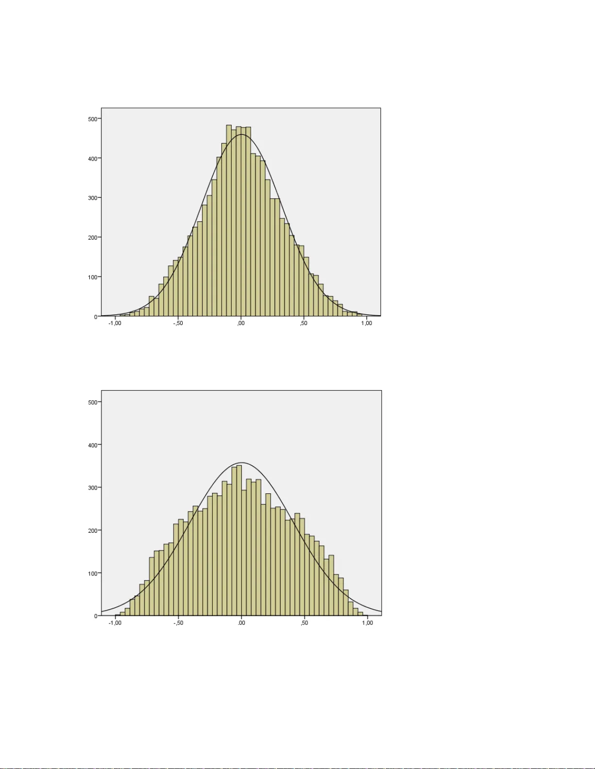
1 The factor para dox: Comm on factors can be correlated with the variance not accounted for by the comm on factor s! André Beauducel 1 Abstract The case that the factor model does not account for all the covariances of the observed variables is considered. This is a quit e realistic condition because some model error as well as some sampling error should usually occur with empirical data. It is shown that principal components representing co variances not accounted for by the factors of the model can have a non-zero correlation with the common factors of the fac tor model. Non-zero correlations of components representing variance not accounted for by the factor model with common factors were also found in a simulation study. Based on these results it should be concluded that common fac tors can be correlated with variance components representing model error as well as sampling error. In consequence, even when researc hers decide not to represent some small or trivial variance by means of a common factor, these excluded variances can still be part of the model. Keywords: Factor analysis; Principal component analysis; Factor model 1 Institute of Psychology, University of Bonn, Kaiser-Karl-Ring 9, 53111 Bonn, Germany , Email: beauducel@uni-bonn.de 2 1 Introduction The factor model has been developed primarily in psychology and has meanwhile bee n applied to a broad variety of data in many fields, even outside of psyc hology. A merit of the model is that latent variables can be constructed that may explain the covariances between observed variables. The model has been de scribed in several books (e.g., Gorsuch, 1983; Harris, 2001; Harman, 1976; Tabachnick & Fidell, 2007) and seve ral software packages are available for the estimation of the model parameters. Nevertheless, it might not be regarded as a realistic assumption that the factor model fits perfectly to the data (MacCallum, 2003; MacCa llum & Tucker, 1991). MacCallum and Tucker (1991) called the misfit of the factor model in the population model error and they also describe sources of sampling error for the factor model. Both model error and sampling err or might have the effect that the factor model does not account for the complete covariance of observed variables. Whereas Mac Callum (2003) as well as MacCallum and Tucker (1991) were concerned with the consequences of model error and sampling error for the model description and for the estimation of model para meters, the present paper investigates the correlation of the variance not accounted for by the factor model with the co mmon factors. Beauducel (2013) found that the correlation between the variance not accounted for by the principal component model and the common factors is not necessarily zero. This means that variance that is regarded as irrelevant according to principal component anal y sis can be relevant for the common factors. I n contrast, the present p aper investigates the correlation of the variance not accounted for by the factor model with the common factors. Since this variance is not part of the factor model one would expect this variance to be uncorrelated with the common factors. 2 Definitions The defining equation of the common fac tor model is x =  f + e , (1) 3 where x is the random vector of observations of order p , f is the random vector of factor scores of order q , e are the unobservable random error vectors or error factor scores of order p , and  is the factor pattern matrix of order p by q . The common factor sc ores f , and the error factor scores e are assumed to have an expectation zero (  ( x ) = 0,  ( f ) = 0,  ( e ) = 0). The expected variance of the factor scores is one, the covariance between the common factors and the error factors is assumed to be zero (Cov( f , e ) =  ( f e´ ) = 0). The expected covariance matrix of observed variables  can be decomposed into  =  ´ +  2 , (2) where  represents the q by q factor correlation matrix and  2 is a p by p diagonal matrix representing the expected covariance of the error factors e (Cov( e , e ) =  ( e e´ ) =  2 ). Moreover, postmultiplication of Equation 1 with e´ shows that the expected covariance of the error factors with the observed variables is Cov( e, x) =  ( ex ´ ) =  2 , because  ( f e´ ) = 0 . It is assumed that the diagonal of  2 contains only positive values so that  2 is nonsingular. 3 Results 3.1 Correlation with unexplained variance Consider that there is some model error so that the factor model in the population does not account for the covariance of the observed variables completely. This could be written as  =  ´ +  2 +  , (3) with  representing the expectation of the residual covariances. Since the factor model as defined in Equation (2) accounts for all diagona l elements in  , there are only nondiagonal elements in  . The remaining definitions of the factor model are not altered by Equation (3), only the nonze ro nondiagonal elements in  are taken into account. Let  = KVK´ with KK´ = K´K = I be the eigen-decomposition of  , where V is diagonal with the eigenvalues in decreasing order. Since the main-diagonal of  contains only zero values, the trace of V will be zero. Therefore, even when some nondiagonal elements of  are not zero, only the first eigenvalues of  will be positive and some negative eigenvalues will also occur. In the following, only the eigenvectors 4 corresponding to positive eigenvalues are considered. The matrix K * contains only eigenvectors corresponding to positive eigenvalues and V * contains only positive eigenvalues (in descending order), so that N = K * V *1/2 . N is called the loading matrix of the corresponding principal components.  * is the matrix of expected residual covariances reproduced from the principal components with positive eigenva lues, with  * = NN´ = K * V * K * ´ . (4) Accordingly, the corresponding residuals of the observed variables can be decomposed into principal components u , which yields x -  f - e = Nu , (5) with u being orthogonal components with  ( uu ´ ) = I . It follows from Equation (5) and from the definitions of the factor model that  (xf´) =  (  + Nuf´) (6) and that  (xe´) =  (  2 + Nue´) . (7) The following theorem states that when the expected correlation between the error factor scores e and the residual components u is zero, a nonzero expected correlation of the common factors f with u occurs. Theorem 3.1.  (fu´) ≠ 0 if  (eu´) = 0 . Proof. It follows from Equations (5), (6), and (7) that NN´ =  (  - (  + Nuf´)  ´ -  2 - Nue´ -  (  + Nuf´)´ +  ´ -  2 - eu´N´ +  2 ) =  (  -  ´ - Nuf´  ´ -  2 - Nue´ -  ´ -  fu´N´ +  ´ - eu´N´) =  ( - Nuf´  ´ - Nue´ -  fu ´ N´ - eu´N´) . (8) For  (eu´) = 0 Equation (8) can be transformed into NN´ =  ( - Nuf´  ´ -  fu´N´ ) . (9) Equation (9) is true iff  (  fu´) = - 0.5 N . This completes the proof.  Theorem 3.2 specifies the condition for the expected zero correlation of the common factors f with the residual components u . 5 Theorem 3.2.  (fu´) = 0 iff  (eu´) = - 0.5 N . Proof. For  (fu´) = 0 Equation (8) can be transformed into NN´ =  ( - Nue´ - eu´N´ ). (10) Equation (10) is true iff  (eu´) = - 0.5 N . This completes the proof.  Theorem 3.3 specifies that the expected correlation of the variance accounted for by the factor model (  f + e) with the residual components u is not zero. Theorem 3.3.  ((  f + e)u´ ) ≠ 0 . Proof. Equation (8) can be transformed into NN´=  ( - Nu(  f + e)´ - (  f + e)u´N´) . (11) Equation (11) is true iff  ((  f + e)u´) = - 0.5 N . This completes the proof.  The meaning of Theorem 3.3 is that the components u , representing variance not accounted for by the factor model, have a nonzero correlation with the variance accounted for by the factor model. Transformation of Equation 5 revea ls t hat the components u can be calculated as u = (N´N) -1 N´(x -  f - e) . (12) Both f and e are usually unknown due to factor score indeterminacy (Guttman, 1955) so that Equation 12 implies that indeterminacy also holds for u . Thus, in a typical situation of an applied researcher, the correlation of the components re p resenting the variance not accounted for by the factor model with the common factors remains unknown. 3.2 Simulation Study The magnitude of the correlations between the common factors and the components repre senting the residuals cannot be investigated within empirical studies, be cause the population common factor scores and the population error factor scores are unknown. However, in simulation studies population common factor scores and population error factor scores can be fixed a priori so that their correlation with the components representing residuals can be investigated in the population 6 and in the sample. Therefore, a simulation study was conduc ted in order to i nvestigate the size of the correlations between the common fac tors and components representing the variance that is not accounted for by the factor model. It is, moreover possible to investiga t e in the simulation study the case that the residual covariances do not represent model error but sampling error. This is interesting because sampling error should not be systematically related to the common factors. Only the first component representing the variance not accounted for by the fac tor model was considered in this simulation, because the first component will always summarize most of the residual variance and because it will always have a positive eigenvalue. Of course, in most data sets even more than one component with eigenvalues greater than zero will occur. However, it is already informative to investigate the correlation of the first component of residuals with the common factors. The conditions of the small simulation study were the number of case s in the sample (150, 300, 900 cases), the size of the salient loadings (.40, .60, .80), and the number of factors (3, 6 factors). For each of the 18 conditions (3 numbers of cases x 3 loading sizes x 2 number of factors) 1,000 factor analyses were performed with SPSS 18. The population for the models comprised 900,000 cases. As an example the population three-factor model for salient loadings of .40 is present ed in Table 1. Table 1: Three-factor population models based salient loadings of .40 orthogonal variables F1 F2 F3 x 1 .40 .00 .00 x 2 .40 .00 .00 x 3 .40 .00 .00 x 4 .40 .00 .00 x 5 .40 .00 .00 x 6 .00 .40 .00 x 7 .00 .40 .00 x 8 .00 .40 .00 x 9 .00 .40 .00 x 10 .00 .40 .00 x 11 .00 .00 .40 x 12 .00 .00 .40 x 13 .00 .00 .40 x 14 .00 .00 .40 x 15 .00 .00 .40 7 Since orthogonal population models were investigated, Varimax-rotation (Kaiser, 1958) was performed for the 18,000 maximum likelihood factor analyses based on the random samples drawn from the population. The factor analyses were based on the correlations of the observe d variables. The mean eigenvalues of the first components representing the correlations not accounted for by the factor model were larger for smaller sample sizes and for smaller salient loading siz es (see Table 2). This was to be expected, since no model error was present in the population models so that the first component should only represent residual correlations that are due to s ampling error. Table 2: Means and standard deviations (in brackets) of eigenvalues of the first principal component calculated from the residual correlations Salient loading Sample size M (SD) M (SD) .40 150 .66 (. 67) 2.02 (1.02) 300 .17 (. 13) .54 (. 51) 900 .05 (. 01) .11 (. 02) .60 150 .16 (. 04) .36 (. 07) 300 .08 (. 02) .17 (. 03) 900 .02 (. 01) .05 (. 01) .80 150 .08 (. 03) .20 (. 04) 300 .04 (. 01) .10 (. 02) 900 .01 (. 00) .03 (. 01) The distributions of the correlations of the f irst component representing the residual correlations of factor analysis with the first common factor are presented in Fig u re 1. Although the distributions are quite symmetric, the kurtosis of the distribution of corre lat ions was a bit smaller when based on the six-factor solutions (Figure 1 A) than the kurtosis of the distribution of correlations when based on the three-factor solutions (Figure 1 B). 3 factors 6 factors 8 (A) (B) Figure 1. Histogram of correlations between the f irst component of residuals with the first common factor in the analysis based on three factors (A) a nd th e analysis based on six factors (B). frequency r frequency r 9 Mo re importantly, the whole range of positive and negative correlations occurred: 17,1% of the correlations had an absolute size greater than .80 for the three-factor solutions and 2,9% of the correlations had an absolute size greater than .80 for the six-factor solutions. In order to provide a more complete description of the effects of the conditions of the simulation study, the r oot m ean squared correlation (RMSC) of the first component representing the residual correlations from factor analysis with the common factors was computed. No results of significance tests were reported because – due to the large sample size of the simulation study – all condition main effects and all interactions were significant in ANOVA at the .001 level. The size of the relevant effects can be depicted from Figure 2: The RMSC was larger than .50 for the three factor solutions and was about .40 for the six factor solutions. Thus, the RMSC decrea s es with the number of factors, but it does not decrease with sample size and with the size of the salient loadings. Figure 2. Root mean squared correlation (RMS) of the first compone nt representing residuals of factor analysis with common factors for the conditions of the simulation. Standard errors were smaller than .01 and were therefore not presented. 0,00 0,10 0,20 0,30 0,40 0,50 0,60 0,70 150 300 900 150 300 900 150 300 900 RMS Sample size 3 factors 6 factors Loading size .40 .60 .80 10 Discussion The correlation of the variance not accounted for by the factor model with the common factors was investigated. Since this unexplained variance is by definition not part of the factor model one would expect components representing this variance to be uncorrelated with the common factors. However, i t was shown algebraica ll y a nd b y means of a simulation study that the common factors can have in fact a nonzero correlation with components representing the variance not accounted for by the factor model. Moreover, the sum of the common factor variance and the error factor variance representing the total variance that is accounted for by the factor model w as shown to have a nonzero correlation with the variance not accounted for by the factor model. According to Theorem 3 the common factors are unc orrelated with the components representing unexplained variance only under a condition implying that the error fac tors h ave a nonzero correlation with the se components. However, since the error factors are aimed at representing unique variances, they should not be correlated with any other v ariance according to the factor model. Moreover, a simulation study revealed that the root mean squared correlation of the first component representing unexplained variance with the common factors was greater than .50 for the three-factor solutions and about .40 for the six-factor solutions. It should be concluded that these correlations cannot be regarded as being virtually zero in general. Since factor anal y sis will nearly always be performed on sample data and since this would always lead to some covariances that are not accounted for by the factor model (MacCallum, 2003; MacCallum & Tucker, 1991), the results presented here will be relevant for most applications of factor analysis. Overall, i t seems that further methodologica l d evelopments are necessary in order to provide a form of factor analysis that avoids the problem that has been demonstrated here. Meanwhile, severe caution is recommended with respect to the interpretation of common factors as representing only the common variance of the observed variables. In contrast, it is likely that the common factors are correlated with the variance that is not accounted for by the factors. 11 References Beauducel, A. (2013). A note on unwanted variance in explorator y factor models. Communications in Statistics – Theory and Methods 42:561-565. Gorsuch, R.L. (1983). Factor analysis (2nd ed.). Hillsdale, NJ: Erlbaum. Guttman, L. (1955). The determinacy of factor score matrices with applica ti ons for five other problems of common factor theory. British Journal of Statistical Psychology 8:65-82. Harman, H.H. (1976). Modern factor analysis (3rd ed.). Chicago: The University of Chicago Press. Harris, R.J. (2001). A primer of multivariate statistics (3rd ed.). Hillsdale, NJ: Erlbaum. Kaiser, H.F. (1958). The varimax criterion for analytic rotation in factor a nalysis. Psy chometrika 23:187-200. MacCallum, R.C. (2003). Working with imperfect models. Multivariate Behavioral Research 38:113-139. MacCallum, R.C. & Tucker, L.R. (1991). Representing sources of error in the common-factor model: Implications for theory and practice. Psychological Bulletin 109:502-511. Ta bach nick , B .G. & F ide ll, L. S. ( 2007 ). Us ing mul tiv aria te sta ti stic s ( 5th Ed. ). Bost on, MA : Pea rso n E duca tio n.