Active Sampler: Light-weight Accelerator for Complex Data Analytics at Scale

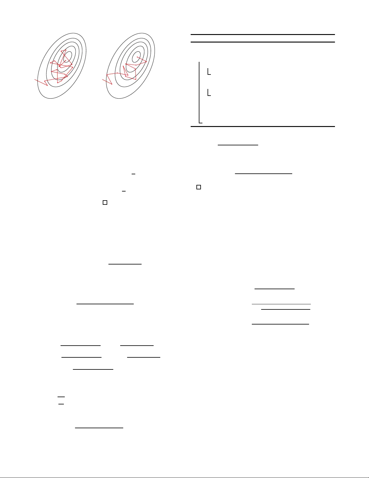
Active Sampler: Light-weight Accelerator f or Complex Data An alytics at Scale Jiny ang Gao ‡ H. V . J agadish § Beng Chin Ooi ‡ ‡ National University o f Singapore § Unive rsity of Michigan ‡ { jiny ang .gao , ooibc } @comp .n us.edu.sg § jag@umich.ed u ABSTRA CT Recent years hav e witnessed amazing outcomes from “Big Models” trained b y “Big D ata”. Most p opular algori thms for mod el training are iterativ e. Due to the surging volumes of data, w e can usually afford to pro cess only a fraction of the training data in each iteration. T ypically , th e data are either un iformly sampled or sequential ly accessed. In this p ap er, we study how the data access pattern can affect mod el training. W e propose an A ctive Sampler al- gorithm, where training d ata with more “learning v alue” to the mo del are sampled more frequently . The goal is to focus training effort on v aluable instances near the classifi- cation b oundaries, rather than evident cases, n oisy data or outliers. W e show th e correctness and optimality of Active Sampler in th eory , and t hen d evel op a ligh t-weig ht vector- ized implementation. Active Sampler is orthogonal to most approac hes optimizing th e efficiency of large-scal e data ana- lytics, and can be applied to most analytics models trained by stochastic gradien t descent (SGD) algo rithm. Extensive exp erimental ev aluations demonstrate th at Active Sampler can speed up the training pro cedure of SV M, feature selec- tion and deep learning, for comparable training qualit y by 1.6-2.2x. 1. INTR ODUCTION W e live in an age of ever-increasing size and complexit y of “Big Data”. T o understand the data and d ecipher the information that tru ly counts, many adv anced large-scale mac hine learning mo d els hav e b een devised, from million- dimension linear mo dels (e.g. Logistic Regression [9], Sup- p ort V ector Machine [25], feature selection [16, 31], Princi- pal Component Analysis [10]) to complex models like D eep Neural Netw orks [4] or topic mo dels [8]. While these mo d- els have demonstrated v alue for a wide spectrum of appli- cations [18, 16, 12], th eir complexit y causes the training cost to increase dramatically with the surging vo lume of data. This difficult y with scale severely affects the viabil- it y of man y a dv anced models on industry-scale applications. Consequently , accelerating the training p rocedu re of those “Big Mo dels” on “Big D ata” has attracted a great deal of interes t. All the models menti oned in the preceding paragraph, and man y others, can b e formulated as minimizing a spe- cific ob jective function based on a set of data observ ations, i.e. the Empirical R isk Minimization [26] (ERM) problem. Even though gradient descen t [3, 1] has b een widely used for decades, ev aluating the full gradient ov er all t h e train- ing samples (i.e. batc h gradient descent [29]) is ex tremely (a) Easy (b) Hard Figure 1: Information Gain from T raining Data exp ensive in the preva iling scale of millions of training sam- ples. T o reduce the computational cost at ev ery iteration, Sto c hastic Gradient Descent (SGD) [22, 2] optimizes the ob jective fun ction based on a single random sample at each iteration. Thereby , the computation cost p er iteration is re- duced greatl y , but no w man y mo re iterations a re required to reac h a certain degree of accuracy or finally conver ge [20]. This is b ecause t h e sto chastic gradien t used in eac h itera- tion is highly sensitiv e to the specific random sample chosen. Although the exp ectation of stochastic gradien t is exactly the full gradient, the large v ariance causes the direction of stochastic gradien t to deviate from that of the full gradi- ent, whic h is t h e optimal direction to minimize t h e ob jective function. Some samples may even direct th e mod el to the opp osite of the correct d irection. It has b een sh o wn that reducing the v ariance of stochastic gradien t [27, 11, 23 ] will lead to a muc h faster con vergence rate. A commonly used scheme called Mini-batch S GD [15] is dev eloped for this purp ose: by a ver aging the gradien t from a mini-batch of samples, the v ariance of gradient is signifi- cantl y reduced , at the cost of some increased comput ation p er iteration. The op t imal mini-batch size is determined as a trade-off b etw een the increased computational cost p er it- eration for a larger mini-batch and the increased v ariance (and hence num ber of iterations) for a smaller mini-batch. In this pap er, we seek to furth er optimize the sto chastic gradien t by not merely av eraging gradien ts from more ran- dom samples but rather impro ving the quality of data sam- ples. T o this end, we prop ose a light-w eight SGD accelerator inspired by active learning [24, 21]. In active learning, train- ing data are selected to m ax imize th e “learning v alue”. F or example, t o train a classification mod el, training data p oints near class b oun d aries are more v aluable th an p oints in the interi or of a class. W e adapt the idea of active learning to the SGD optimization context by choosing samples from not a u niform distribut ion ov er the training data but rather a biased distribution from which w e ex p ect to learn more. Figure 1 giv es an example of how different samples can affect the training efficiency . The left side con tains some images of written digits that are very easy to classify . F or these “easy-to-classify” images, most models can classif y them correctly even after a handful of steps. In subsequ ent thousands of iterations or even more, these easy-to-classify images will b e sampled and correctly classi fied with high confidence, contributing almost zero gradient to th e mo del. Consequently , th e t raining time consumed by those easy-to- classify images is largely wa sted. In contrast, the righ t side of Figure 1 contains some images that are hard to classify . By pu tting more effort on those “hard- to-classify” images, the accuracy of mo del may improv e at a faster rate. Based on the ab o ve intuition, w e develop a w eighted sam- pling method called Ac tive Sampler . W e find that to maxi- mize t h e information gain in each iteration, the sample fre- quency for each training sample sh ould b e prop ortional to the estimate of its gradient magnitude. Notw ithstanding the sampler itself is biased, we show that the origi nal ob jectiv e function based on uniform weig ht can still b e correctly min - imized by re-w eighting the gradient of each sample. F rom the view of v ariance reduction, Act ive Sampler also provides ta gradient with the smallest v ariance compared with all w eighted sampling metho ds, including the uniform random sampling. The net result is a system that requires far fewer iterations for m o del con vergence (or to reac h a req uired ac- curacy th reshold). Although optimization metho ds can redu ce t he num b er of iterations, it should also b e noted that they may introduce additional compu tation cost in eac h iteration. There ha ve b een a great amount of researc h works [23, 11 , 19] fo cus- ing on accelerating SGD. Theoreticall y , these metho ds h a ve significan tly faster conv ergence rate. While Momen tum and AdaGrad [6] metho ds hav e shown th eir effectiveness and hav e b een integrated into practical S GD solver, most meth- ods are far from b eing used in practice due to their signifi- cant additional computation cost. F or ex ample, the cost of SVRG [11] per iteration is at least three t imes the cost of standard SGD per iteration. As noted in [19], mini- b atc h SGD still dominates in most cases, du e to its light-w eight computation and goo d vectori zation. T o make Active Sampler as efficient as p ossible in prac- tice, th e design principle is to reduce th e ov erhead inv olve d in each iteration. In the actual implementation, w e u se lots of existing knowledge to approximate the information that needs additional compu tation cost, and the sampling dis- tribution is decided by the gradien t magnitu d e in previous iterations. T o ev aluating the gradient magnitude for eac h sample, an effective scheme is app lied to av oid the explicit calculation of the gradien t of eac h sample. This sc heme makes it p ossible that t h e comp u tation for multiple samples can still b e efficiently vectorized. Moreo ver, the computa- tion cost is only O ( m + l ) for a m × l p arameter matrix. Therefore, for Active S ampler, the computation ov erhead introduced in each iteration is ligh t-weig ht, considering its significan t contribution in reducing the num b er of total it- erations. The contributions of our work are summarized as follo ws: • W e prop ose a general SGD accelerator, called Active Sampler, where more informativ e training data is sam- pled more frequently for mo del training. W e formalize T able 1: Examples of ER M Applications Algorithm f w ( x ) L ( f w ( x ) , y ) ρ f ( w ) Linear Regr ession w T x ( y − f w ( x )) 2 0 or λ k w k 2 2 Hinge-loss SVM w T x max(0 , 1 − f w ( x ) ∗ y ) 0 or λ k w k 2 2 Logistic Regre ssion w T x log(1 + exp ( − f w ( x ) ∗ y )) 0 or λ k w k 2 2 F eat ure Selection w T x log(1 + exp ( − f w ( x ) ∗ y )) λ k w k 1 Neural Net work complex log(1 + exp ( − f w ( x ) ∗ y )) 0 or λ k w k 2 2 PCA ww T x - x k f w ( x ) k 2 2 0 the problem as S GD optimization for ERM with weigh ted sampling, and show that the Active Sampler has the largest information gain and th e smallest v ariance among all weigh ted sampling solutions. • W e develop a light-w eigh t and fully vectorized algorithm for A ctive Sampler, making the computation cost of A c- tive S amp ler in eac h iteration comparable to the naiv e mini-batch S GD . • W e implemen t the Active S ampler framework and ev al- uate its p erformance on three popular mac hine learning algorithms: SVM, feature selection and deep neu ral net- w ork. Active Sampler reduces th e num b er of iterations to reach a certain accuracy by half, while only consuming 10%-20% additional computation cost in eac h iteration. In short, Active S ampler sp eeds up the training pro ce- dure by more than 1.6x. The remainder of this pap er is organized as follo ws. W e first introduce the backgro und in Section 2. Then we pro- p ose th e Active S ampler, show its effectiveness in th eory and discuss its practical implementation issues in Section 3. The exp erimental results are d iscussed in Section 4. Finally , we review ab out the related works in Section 5 and conclude at Section 6. 2. PRELIMIN ARIES In this section, we first introduce the Empirical Risk Mini- mization (ERM) framework, and sh ow its connection to data analytics mod els. Then we d escribe the stochastic gradien t descent algorithm, a general solver for the ERM problem, whic h w e aim to impro ve up on in th is wor k. 2.1 Empirical Risk Minimization Empirical Risk Minimization (ERM) is a principle in the statistical learning theory which forms the b asis for defin- ing a family of analytics models. F rom the view of ERM, the centra l idea in machine learning is to learn a mo del and use it to approximate the data. The difference b etw een th e approximatio n and the real data is th en measured b y a loss function, which should b e minimized by tuning the param- eters of the mo del. F or the sake of simplicity , in this work w e formali ze ERM from th e sup ervised learning p ersp ec- tive, where eac h t raining instance is a pair h x , y i consisting of con tent x and lab el y . F or u n sup ervised problems, lab el y is a null term Φ, and d ata can b e represen ted as h x , Φ i . Definition 1 (Loss F unction) Given a data i nstanc e r ep- r esente d as h x , y i , and a mo del hyp othesis f w (i.e. a mo del f with p ar ameter w ), the loss function L ( f w ( x ) , y ) is a dis- agr e ement me asur e function b etwe en the mo del appr oxima- tion (i.e. pr e diction) f w ( x ) and the actual lab el y . Here w e shall giv e seve ral examples on the loss measures that are commonly u sed. F or hard classification problems, the loss measure function can be written as: L ( f w ( x ) , y ) = I [ f w ( x ) 6 = y ]. F or linear regression, the loss measure func- tion can be written as: L ( f w ( x ) , y ) = k f w ( x ) − y k 2 2 . F or general linear mo dels where f w ( x ) = w T x and y = ± 1, if th e loss measure is L ( f w ( x ) , y ) = max(0 , 1 − f w ( x ) ∗ y ), then the mo del is a h inge-loss SV M; if the loss measure is the log logistic function L ( f w ( x ) , y ) = log (1+ exp ( − f w ( x ) ∗ y )), then the mo del is a logistic regression. F or PCA, by using w to denote the low rank pro jection matrix, th e problem can b e form ulated as f w ( x ) = ww T x − x , and L ( f w ( x ) , y ) = k f w ( x ) k 2 2 . After defining the measure of disagreemen t b etw een mod el output and target lab el, the ultimate goal of learning is natu- rally to minimize th e total disagreemen t by tuning the mo del parameters. This is called Risk Minimi zation [26], which is defined as follo ws: Definition 2 (Risk Minimization) L et P h x ,y i to b e the distribution of data, the risk asso ciate d with mo del hyp othe- sis f w is define d as the exp e ctation of the loss for the p ote n- tial data distribution: R ( f w ) = E [ L ( f w ( x ) , y )] = Z L ( f w ( x ) , y ) d P h x ,y i (1) The go al of le arning algorithms is to find the p ar ameter w that minimi zes the risk: argmin w R ( f w ) (2) How ever, in general, R ( f w ) cann ot b e directly minimized since the exact latent data distribut ion P h x ,y i is unkn o wn. Instead, the common wa y is to use the distribution of train- ing d ata to appro ximate P h x ,y i . Therefore, the Empiric al Risk [26] is used as the optimization target. Definition 3 (Empirical Risk) The empiric al risk i s de- fine d as the aver age of loss on the tr aining set with n in- stanc es. R emp ( f w ) = 1 n X i L ( f w ( x i ) , y i ) (3) T o simplify the notation, we use L ( w ) to denote R emp ( f w ) . According to the VC-dimension theory [26], the difference b etw een real risk and empirical risk may b e large when th e mod el hyp oth esis f w is to o complex while the size of training data n is not large enough. This phenomenon is called ov er- fitting. T o preven t o ve r-fitting, the empirical risk is often regularized to p enalize the complexit y of model f w : Definition 4 (ERM with Re gularization) The empi ri- c al risk with r e gularization is define d as the aver age of loss function on the tr aining set, plus a p enalty r e gularization term ρ f ( w ) b ase d on the c omplexity of the mo del f w . R r eg − emp ( f w ) = L ( w ) + ρ f ( w ) (4) In ERM with r e gularization, the go al of le arning algorithm is to minim i ze the empiric al risk with r e gularization, i .e., argmin w R r eg − emp ( f w ) (5) F or most app lications, w e u se the l 2 -norm of parameter λ k w k 2 2 as the regularization function ρ f ( w ). This is actu- ally a Gaussian prior ov er the parameter distribut ion from T able 2: Common Notations Notation Meaning h x , y i training instance w mod el parameters f w ( x ) mod el prediction for data x L ( f w ( x ) , y ) loss on instance h x , y i L ( w ) empirical risk ρ f ( w ) regularization term ∇ w gradien t op erator ∇ w L ( w ) batch gradient g i ( w ) stochastic gradient p i sampling p rob ab ility for h x i , y i i V a r ( g i ( w )) scalar v ariance of g i ( w ) the Ba yesian v iew. F o r feature selection metho ds such as Lasso [16], t he l 1 -norm regularization λ k w k 1 is used to se- lect those sparse features. W e list some examples of analytics mo dels from ERM fam- ily in T able 1, and sho w th eir connections. 2.2 Stochastic Gradient Descent T o optimize the ERM problem describ ed in Equation 5, batch gradient descent metho d is used to iteratively alter the parameter tow ards t h e fastest direction to minimize the ob jective function. By d efining the step size using the learn- ing rate η , batch gradient descent m eth od uses the follo wing up dating rule to optimize the parameter: w new = w − η ∇ w ( L ( w ) + ρ f ( w )) = w − η ∇ w ρ f ( w ) − η n X i ∇ w L ( f w ( x i ) , y i ) (6) As can b e observed from Equation 6, w e n eed to eva luate t he gradien ts ∇ w L ( f w ( x i ) , y i ) for all training instances at each step, making the computation cost of ∇ w L ( w ) extremely exp ensive. T o av oid this cost, stochastic gradient metho ds use an inexact gradien t whic h is estimated from random samples. Definition 5 (Stochastic Gradient Descent) I n sto cha- stic gr adient desc ent, the true gr adient ∇ w L ( w ) is appr oxi- mate d by a sto chastic gr adient g i ( w ) . w new = w − η ∇ w ρ f ( w ) − η g i ( w ) (7) T aking g i ( w ) as a r andom variable, the exp e ctation of g i ( w ) should e qual to the gr adi ent of L ( w ) , i. e. E i [ g i ( w )] = ∇ w L ( w ) (8) In the standar d SGD algorithm, g i ( w ) i s obtaine d by sim pl y evaluating the gr adient at a r andom single instanc e i : g i ( w ) = ∇ w L ( f w ( x i ) , y i ) (9) wher e i is r andomly dr awn fr om { 1 , ..., n } , and the sampling pr ob ability p i for e ach instanc e i is 1 /n . The sc alar varianc e of sto chastic gr adient is denote d as V a r ( g i ( w )) , define d by E i [ k g i ( w ) − ∇ w L ( w ) k 2 2 ] , w hi ch is a sc alar inste ad of the c o- varianc e matrix. T able 2 lists most of the imp ortan t notations used throu gh - out th is pap er. Un less otherwise sp ecified, v ariance used in the pap er refers to the scalar vari ance. Intuitively , th e re- quirement E i [ g i ( w )] = ∇ w L ( w ) is t o guaran tee that the SGD algorithms will conv erge at the optimal p oin t [20], as the ex p ectation of up date in SGD will b e a zero vector at t h e p oint where b atc h gradient descent algorithm con- verge s. Obviously , the standard SGD algorithm satisfies this requirement. E i [ g i ( w )] = X i p i g i ( w ) = X i 1 n ∇ w L ( f w ( x i ) , y i ) = ∇ w 1 n X i L ( f w ( x i ) , y i ) = ∇ w L ( w ) (10) Although the training cost p er iteration for S GD is ex- tremely ligh t-w eight compared to th e b atc h gradien t algo- rithm, the main drawbac k of SGD is th at g i ( w ) is n ot the exact ∇ w L ( w ). Therefore, t he direction of the stochastic gradien t g i ( w ) differs from the optimal direction ∇ w L ( w ). This phenomenon causes SGD algorithm to b e less efficien t and take more iterations to conv erge or reac h a certain ac- curacy . It has been shown by [27, 11, 23] that simply re- ducing t he va riance of stochastic gradient will increase the conv ergence rate of SGD algorithms. Ho w ever, most v ari- ance red uction techniques require add itional computation cost compared with th e standard SGD. In essence, there is a trade-off b etw een the num b er of iterations required to reac h a certain accuracy and th e computational cost p er iteration. Therefore, the main goal of optimizing SGD algorithm is to reduce th e v ariance of g i ( w ), while keeping the compu tation of g i ( w ) light-w eight. 3. A CTIVE SAMPLER 3.1 Over view In th is pap er, we revisit the SGD algorithm from a brand new an gle – the information gain of th e mo del at each it- eration. W e can regard the S GD algorithm as an active learning pro cedure which sequ entia lly takes samples from the dataset and refi nes its mo del. Naturally , training the mod el using samples with more information w ould facilitate faster impro vemen t of the mod el. W e term our we ighted sampling strategy as A ctive Sampler . The in tuition here is that a larger number of training samples are not helpful for refining the mo del (or at least not helpful at a certain train- ing stage), including data that are too evident to predict, data that are noisy , and d ata that have just been visited. By simply skipping t hese samples, w e can sa ve a significant amount of training time. In contrast, the samples that are close to the b order of class ma y b e very helpful to refin e the mod el (or even define th e mod el in some cases such as SVM). This idea is very similar t o active learning bu t with a ma jor difference – the ob jective of active learning is to redu ce the num ber of training samples, while th e ob jective of active sampling is to reduce th e number of training iterations. T o exploit information gain as a means to sp eed u p SGD training, th ree issues ha ve to b e addressed: (1) define what is t he information gain for mo d el training from each t raining sample; (2) adapt th e Active S ampler into the SGD frame- w ork and stud y how information gain can help sp eeding u p SGD; (3) design a ligh t-we ight implementation that can be Figure 2: Uncertaint y applied to real systems. W e shall address these three issues in th e follo wing subsections. 3.2 Inf ormation Gain In this subsection, we define the information gain directly follo wing the basic in tuition from the training of typical soft margin classifiers. Later, w e will fit this initial idea into a formal SGD framew ork and provide a rigor ous th eoretical analysis that illustrates how this strategy can b enefi t the p erformance of SGD for all sorts of ER M problems in the next subsection. In soft margin classifiers, instead of giving a single la- b el as the p rediction, the classifier outputs a p robabilistic distribution ov er laten t lab els. Recently prop osed classifica- tion algori thms (e.g. Lasso, Neural Net wo rk and Soft SVM etc.) are typically trained as soft margin classifiers, since the conti nuous optimization is muc h efficient than the discrete optimization, which is a NP-Hard problem. Definition 6 (Soft Ma rgin C lassifier) Given a pr e dictor f w , the soft pr ob abilistic classifier is define d by using lo g l o- gistic function as the loss function, i. e. L ( f w ( x ) , y ) = log (1 + exp ( − f w ( x ) ∗ y )) (11) Obviously, al l algorithms i n T able 1 using the lo gistic loss function ar e soft mar gin classifiers. The r ationale i s that the lo gistic function is use d to tr ansfer the pr e diction f w ∈ R to a classific ation pr ob ability, i.e. P r ( y | f w ( x )) = 1 / (1 + exp ( − f w ( x ) ∗ y )) (12) Then the lo g-likeliho o d log P r ( y | f w ( x )) is maximi ze d, i. e. the loss is log(1 + exp ( − f w ( x ) ∗ y )) . Now , let us analyze th e p ossible factor s that may affect the information gain of a model from eac h training sam- ple. First, from the v iew of active learning, the information gain by rev ealing a label which can be easily predicted is very limited. This is also tru e for the SGD algorithm – visiting a sample that th e model can alw a ys classify cor- rectly is not h elpful, as the loss cannot b e further reduced if the loss is already close to 0. A mo del can only learn from samples which are un certain in p rediction. Figure 2 sho ws an example to illustrate why uncertaint y helps the mod el to improv e: the images on the left are very easy to predict, and therefore P r ( y | f w ( x )) is almost 100%. As a re- sult, the loss L ( f w ( x ) , y ) for each of those images is almost zero and has little ro om for further optimization. I n con- trast, the images on the right is muc h h arder to pred ict. By selecting them as samples for optimization purp ose, th e loss L ( f w ( x ) , y ) on those samples could b e significantly reduced and the a verage performance of mo del is h ence improv ed. Figure 3: Significance In information theory [26], t he information gain by reveal- ing a random v ariable is usually defined as the entrop y of that rand om v ariable: Definition 7 (Uncertain ty) The unc ertainty of a tr ain- ing instanc e x i for a mo del f w is define d as the entr opy of the f w ( x i ) , i.e. U ( w , x i ) = − X y P r ( y | f w ( x i )) log P r ( y | f w ( x i )) (13) Second, n ot all the training instances contribute eq u ally to the mod el p erformance. F or examp le, though the mo del may alw a ys b e uncertain ab out th e label for noisy data, this d oes not mean that noisy d ata are more helpful to improve the mod el p erformance. This is b ecause the uncertaint y mea- sure only ev aluates the information inside the lab el, but n ot its con tribution to the mo del. Therefore, we introduce an- other measure called signi fic anc e to ev aluate the efficiency of information transfer from the data to the mo del. Intuitiv ely , the output of a noisy instance is not sensitiv e to the c hange of the parameter. When the outpu t of a data instance is sensitiv e t o the c hange of p arameter, its loss will b e signif- ican tly reduced even with tiny c hanges of the parameter, whic h provides a clear instruct ion on how to reduce the loss by tun ing the p arameter. The right h and side of Figure 3 sho ws the images that are noisy and with less significance. Definition 8 (Significance) The signific anc e of a tr ain- ing instanc e x i for a mo del f w is define d as its sensitivity to p ar ameter change: S ( w , x i ) = k∇ w f w ( x i ) k 2 (14) k∇ w f w ( x i ) k 2 is the maximal change of f w ( x i ) when the p a- r ameter w changes an unit di stanc e. Here, w e give a comp arison b etw een un certain ty and sig- nificance: uncertaint y measures the exp ectation of accuracy on the current mod el, while significance measures th e p oten- tial improve ment of accuracy by tuning the mo del. There- fore, instances th at are easy to classify usually hav e lo w un - certain ty but high significance; noisy instances usually h a ve high u ncertaint y but low significance, while v aluable b order instances that hav e not b een well learned usually h a ve b oth high un certain ty an d high significance. Third, the information gain in one iteration may o ver- lap with the information obtained in earlier training step s. F or example, v isiting the training instance that has just b een trained usu ally does not p ro vide extra information th an what has b een derived in the previous visit. H o w ever, for a completely new instance that hasn’t b een trained, there may b e no o verlap b etw een the information gain and information in previous steps. Therefore, we use the visiting interv al to measure the effect of information ov erlap: Definition 9 (In terv al) The vi siting interval I ( w , x i ) of a tr aini ng i nstanc e x i for a mo del f w is define d as the numb er of iter ations sinc e the l ast time x i was use d in tr aining. A lar ger interval pr ovides l ess information overlap and mor e pur e information gain. Com bining all th e th ree factors together, w e d efine the information gain of model f w from training instance x i as I G ( w , x i ): I G ( w , x i ) = U ( w , x i ) ∗ S ( w , x i ) ∗ I ( w , x i ) (15) The ob jective of our A ctive Sampler is to choose th e training instance x i with the larges t I G ( w , x i ). Theorem 1 (Information Gain M aximization) B y ch- o osing the lar gest I G ( w , x i ) i n e ach iter ation, the sampling fr e quency p i of e ach tr aining instanc e x i should b e pr op or- tional to its exp e ctation of the gr adient magnitude, i.e. p i = E y [ k∇ w L ( f w ( x i ) , y ) k 2 ] P i E y [ k∇ w L ( f w ( x i ) , y ) k 2 ] (16) Pr oof Sketch: At eac h iteration, I G ( w , x i ) for each in- stance will increase U ( w , x i ) * S ( w , x i ), and the instance with the largest I G ( w , x i ) will b e selected as sample. A fter an instance is sampled, its I G ( w , x i ) will b e set to zero as its I ( w , x i ) b ecomes zero. Therefore, as the num ber of itera- tions gro ws, the sampling frequency for eac h instance should b e prop ortional to its U ( w , x i ) * S ( w , x i ), considering that the largest I G ( w , x i ) selected in each iteration should has a similar v alue. Meanwhile, E y [ k∇ w L ( f w ( x i ) , y ) k 2 ] = P y P r ( y | f w ( x i )) k∇ w L ( f w ( x i ) , y ) k 2 = P y P r ( y | f w ( x i )) ∂ ∂ f w ( x i ) L ( f w ( x i ) , y ) k∇ w f w ( x i ) k 2 = P y ( P r ( y | f w ( x i )) ∗ log P r ( y | f w ( x i ))) k∇ w f w ( x i ) k 2 = U ( w , x i ) ∗ S ( w , x i ) (17) 3.3 W eighted SGD Algorithm and Analysis While the ab ov e intuitio n suggests that different training instances should b e sampled at different frequ encies, directly changi ng t he sampling frequency will result in a bias in the target of an optimization. E i [ g i ( w )] = X i p i g i ( w ) = ∇ w X i p i L ( f w ( x i ) , y i ) (18) The loss function to b e minimized is P i p i L ( f w ( x i ) , y i ) in- stead of P i 1 n L ( f w ( x i ) , y i ). The w eigh t for each training instance is unequ al, whic h may affect the accuracy of the mod el. F or this reason, using ∇ w L ( f w ( x i ) , y i ) directly as g i ( w ) is inappropriate. Instead, we should guarantee that E i [ g i ( w )] is ∇ w L ( w ). Theorem 2 (W eighted SGD) Gi ven any sampling dis- tribution { p 1 , . .., p i , . .., p n } , to get a SGD algorithm that optimizes L ( w ) , g i ( w ) should b e r e-weighte d to ∇ w L ( f w ( x i ) ,y i ) n ∗ p i . Standard SGD Active Sampler Same Sampling Probability V aried Gradient Magnitude V aried Sampling Probability Same Gradient Magnitude Figure 4: Comparison with standard SGD Pr oof. T o get a SGD algorithm that optimizes L ( w ), we need E i [ g i ( w )] to b e ∇ w L ( w ). By scaling g i ( w ) w i times and solve E i [ g i ( w )] = ∇ w L ( w ), w e hav e: E i [ g i ( w )] = ∇ w L ( w ) ⇒ E i [ w i ∇ w L ( f w ( x i ) , y i )] = ∇ w L ( w ) ⇒ X i p i w i ∇ w L ( f w ( x i ) , y i ) = X i 1 n ∇ w L ( f w ( x i ) , y i ) ⇒ p i w i = 1 n (19) Therefore, w i = 1 / ( n ∗ p i ). Next, we show that setting p i prop ortional to the gradient magnitude will minimize the v ariance in stochastic gradient g i ( w ) in all w eighted sampling solutions that E i [ g i ( w )] = ∇ w L ( w ). Theorem 3 (Optimal W eigh ted SGD) L et p i denote the sampling pr ob ability of tr aining instanc e h x i , y i i i n a weighte d SGD al gorithm wher e E i [ g i ( w )] = ∇ w L ( w ) . g i ( w ) b e c omes a sto chast ic gr adient with value ∇ w L ( f w ( x i ) ,y i ) n ∗ p i with sampling pr ob ability p i . T o get the weighte d SGD algorithm with the smal l est varianc e of sto chastic gr adient (i . e. V ar ( g i ( w )) ), for e ach instanc e, p i should b e pr op ortional to its magnitude of sto chastic gr adient k∇ w L ( f w ( x i ) , y i ) k 2 . p i = k∇ w L ( f w ( x i ) , y i ) k 2 P i k∇ w L ( f w ( x i ) , y i ) k 2 (20) Pr oof. V a r ( g i ( w )) = E i [ k g i ( w ) k 2 2 ] − k E i [ g i ( w )] k 2 2 = E i [ k∇ w L ( f w ( x i ) ,y i ) k 2 2 ( np i ) 2 ] − k E i [ ∇ w L ( f w ( x i ) ,y i ) np i ] k 2 2 = P i p i k∇ w L ( f w ( x i ) ,y i ) k 2 2 ( np i ) 2 − k P i p i ∇ w L ( f w ( x i ) ,y i ) np i k 2 2 = P i k∇ w L ( f w ( x i ) ,y i ) k 2 2 n 2 p i − k∇ w L ( w ) k 2 2 (21) T o minimize V ar ( g i ( w )) by tuning p i , sub jecting to P i p i = 1, according to Lagrange m ultiplier metho d, w e hav e: ß ∂ ∂ p i ( V ar ( g i ( w )) + λ ( P i p i − 1)) = 0 ∂ ∂ λ ( V ar ( g i ( w )) + λ ( P i p i − 1)) = 0 (22) by solving Equation 22, w e have : λ − k∇ w L ( f w ( x i ) , y i ) k 2 2 ( np i ) 2 = 0 (23) Algorithm 1: Op t imal W eighted SGD Input : Initial w 0 , T Output : Final w T 1 for t = 1 , ..., T do 2 foreac h i = 1 , ..., n do 3 Gr ad [ i ] = k∇ w L ( f w ( x i ) , y i ) k 2 ; 4 S umGr a d = P i Gr ad [ i ]; 5 foreac h i = 1 , ..., n do 6 p i = Gr ad [ i ] /S umGr ad ; 7 sample i from { 1 , ..., n } based on distribution { p 1 , ..., p n } ; 8 g i ( w ) = ∇ w L ( f w ( x i ) , y i ) /np i ; 9 w t = w t − 1 − η ∇ w ρ f ( w ) − η g i ( w ); Therefore, k∇ w L ( f w ( x i ) ,y i ) k 2 2 ( np i ) 2 is a constant val ue for all train- ing instances, whic h means k∇ w L ( f w ( x i ) , y i ) k 2 is prop or- tional to p i . Considering that P i p i = 1, w e h a ve: p i = k∇ w L ( f w ( x i ) , y i ) k 2 P i k∇ w L ( f w ( x i ) , y i ) k 2 (24) Theorem 3 can b e view ed as a refined v ersion of Theo- rem 1 when label y is observed. Theorem 3 gives a rigorous explanation ab out our previous intuition from the v ariance reduction v iew of SGD optimization. Note that this result makes no assumptions ab out th e soft margin classification and applies to all sorts of ERM problems. Algorithm 1 describes th e optimal we ighted SGD algorithm, where the computation cost in eac h iteration will be optimized in the next subsection. Another insight we observ e from Theorem 3 is that in order to m in imize the vari ance of SGD by using weigh ted sampling, g i ( w ) should hav e the exact same magnitud e for all instances. k g i ( w ) k 2 = k ∇ w L ( f w ( x i ) , y i ) np i k 2 = k∇ w L ( f w ( x i ) , y i ) k 2 n ∗ k∇ w L ( f w ( x i ) ,y i ) k 2 P i k∇ w L ( f w ( x i ) ,y i ) k 2 = P i k∇ w L ( f w ( x i ) , y i ) k 2 n (25) This suggests t hat only the direction of th e stochastic gra- dient is determined by the training instance. F urther, the step size (i.e. the magnitude of η g i ( w )) is of no consequence to the t raining in stance and is decided by the global learning rate. As a result, the change of p arameter in Active Sampler is muc h more steady than th e stand ard SGD. This prop erty agrees with the original purp ose of gradient d escen t meth- ods, as the gradien t only indicates the fastest direction to minimize the ob jective loss function, without any ind ication on the step size. Fig ure 4 shows the comparison b etw een standard S GD and Active Sampler. F or stand ard SGD, all training instances hav e the same sampling probability , while th eir gradient magnitudes var y . F or Active Sampler, all training instances ha ve the same gradient magnitude, while their sampling probabilities v ary . Both metho ds have the same exp ectation of gradient, h ow ever, Active Sampler Reinfor cement stage for Sample from whole datase t: Interval is proportional to the size of dat aset Sample from partial datase t at each stage: Interval is proportional to the size of partial datase t : Samples with more accurate prediction Reinfor cement stage for Figure 5: History Reinforcement has a smaller var iance, resulting in a faster and more stable conv ergence pro cess. 3.4 Practical Implementation Issues As discussed in Section 2, the main goal of optimizing the SGD algorithm is to reduce the v ariance of g i ( w ), while keeping the computation cost p er iteration light-w eight. W e hav e already sho wn how to minimize the v ariance of g i ( w ) by using the Active Sampler. In this subsection, we will discuss some practical issues in implementing Active Sam- pler onto real systems, which may significan tly affect the computation time in each iteration. 3.4.1 Sampling base d on Hi story The probabilistic distribution describ ed in Theorem 3 can indeed minimize the v ariance of the stochastic gradien t. Ho w- ever, u se of th e exact distribution, whic h requires all n gra- dients to b e ev aluated at eac h step, is obviously not practi- cal. Instead, w e can p redict the gradient magnitude for eac h training instances u sing h istorical data. A straightforw ard approac h to the problem is to remember th e magnitude of the latest gradien t of each instance and use it as an approx- imation. Considering th at the actual gradient may change and the historical magnitude is only an approximation, a smoothing term is required. F or example, if one instance contri butes a zero gradient at any iteration of the mo del training when it is sampled, th at sample will never b e vis- ited afterw ard if there is no smoothing, n ot withstanding this instance may b ecome va luable for refi nement of the mod el at later stages. Definition 10 (History Appro ximation) L et t i b e the l at- est step wher e tr aini ng instanc e i is visite d and let w t i denote the p ar ameter value at step t i . The sampling pr ob ability for e ach sample i i n a pr actic al A ctive Sampler with smo othing is define d as: p i = (1 − β ) k∇ w t i L ( f w t i ( x i ) , y i ) k 2 P i k∇ w t i L ( f w t i ( x i ) , y i ) k 2 + β n (26) The scheme ensures that every training instance has at least β times t he a vera ge sampling probabilit y (i.e. 1 /n ) b eing sampled. Algorithm 2 d escribes the A ctive Sampler using the history approxima tion. In each iteration, only its gradien t magnitu d e needs to b e up d ated. W e note th at by using the h istory length to denote the num ber of iterations from the last time an instance is sam- pled, its history approximation b ecomes less accurate with the increase of the h istory length. Mean while, the exp ecta- tion of history length for one instance is 1 /p i , and th e av- erage of p i is 1 /n . Consequen tly , the history app ro ximation will b ecome less accurate when data size b ecomes larger. T o Algorithm 2: AS SGD (Active Sampler SGD) Input : Initial w 0 , T , β , Gr ad [], S umGr a d = P i Gr ad [ i ] Output : Final w T 1 for t = 1 , ..., T do 2 sample i from { 1 , ..., n } based on distribution { p 1 , ..., p n } where p i = β /n + (1 − β ) Gr ad [ i ] /S umGr a d ; 3 g i ( w ) = ∇ w L ( f w ( x i ) , y i ) /np i ; 4 w t = w t − 1 − η ∇ w ρ f ( w ) − η g i ( w ); 5 S umGr a d = S umGr a d − Gr ad [ i ]; 6 Gr ad [ i ] = k∇ w L ( f w ( x i ) , y i ) k 2 ; 7 S umGr a d = S umGr a d + Gr ad [ i ]; address this issue, we prop ose History R einfor c ement , whose key idea is illustrated in Figure 5. History Reinforcemen t al- gorithm trains the mo del using a set of stages, eac h of which conta ins a large amoun t of SGD iterations. Within a stage, it first samples a subset of training data which con sists of m instances, and th en uses th em as the training set in its SGD iterations. During the training of each stage, t h e sam- pling probability for the instances is n/m times larger than training all the in stances together. Therefore, the approx- imation will b e muc h more accurate except the first time in a stage when one instance is sampled. The only dra w- back of History Reinforcemen t is that it may lead to a bias in th e training of a stage, as only partial d ata are trained. How ever, [15] presents an effective sc heme in an analogous context to redu ce this b ias b y adding a regularizer to limit the change of parameter in one stage. Below , we formally define the concept of His tory Rei nforcement . Definition 11 (History Reinforcement) History R einfor- c ement algorithm c onsists multiple stages . in e ach stage t , it dr aws a subset I t of tr aining i nstanc es, which c ontains m r andom instanc es fr om the whole dataset, and tr ains the mo del w t using g SGD iter ations. The loss function use d in e ach stage is: L ( w t ) = X i ∈ I t L ( f w t i ( x i ) , y i ) m + γ t 2 k w t − 1 − w t k 2 2 (27) wher e γ t is a p ar ameter i n [ 15] c alculate d b ase d on m , t and V a r ( g i ( w )) . The correctness and effectiveness of this batch training is given in Theorem 1 of [15] (by considering a stage as a batch step ). The av erage num b er of visits for one instance in a stage is g /m . Therefore, 1 − m/g prop ortion of th e iter- ations in a training stage will benefi t from a more accurate approximatio n. I n essence, there is a t rade-off b etw een the bias invo lved by using partial d ata and the accuracy gain in gradien t ap p ro ximation. In tuitively , for larger d atasets, the bias b ecomes less significan t while the accuracy gain by us- ing History Reinforcement becomes more v aluable. On the contra ry , the approxima tion of gradient in small datasets is fairly accurate, and t herefore, directly sampling from t he whole dataset is adv anta geous. 3.4.2 Efficient V ectorized Computation T o red u ce the v ariance of the stochastic gradient, a widely adopted solution is to emplo y mini-batch training, whic h a v- Algorithm 3: ASSGD with History Reinforcement Input : I nitial w 0 , T , m , g Output : Final w T 1 for t = 1 , ..., T do 2 I t = Φ; 3 for i = 1 , ..., m do 4 sample t i uniformly from { 1 , ..., n } − I t ; 5 I t = I t ∪ { t i } ; 6 Compute γ t based on [15]; 7 T rain w t using Algorithm 2 for g iterations, using w t − 1 as initial w 0 , using I t as th e training set, and using ρ f ( w ) + γ t 2 k w t − 1 − w k 2 2 as the regularizatio n function; erages th e sto chastic gradients of multiple training samples. By a vera ging b training samples, the vari ance of gradient can b e reduced by b times ( b is typically b etw een 10 and 1000). Meanwhile, thanks to the effect of vectorized com- putation and the constan t communication cost when th e computations are parallelize d, the training time per itera- tion for mini-b atc h SGD is m uch smaller than b times the training time p er iteration for the standard SGD. There- fore, mini-batch SGD is commonly used in most large-scale optimization problems. A ct ive Sampling is orthogonal to mini-batch SGD, so we could use b oth improv ements simul- taneously . How ev er, t o integrate them together, we need to compute th e av erage of g i ( w ) for b training samples in an efficient vectorized w ay , as w ell as to obtain the gradien t magnitude for eac h training instance. Definition 12 (Mini-batc h SGD / Active Sampler) At e ach iter ation t , mini-b atch SGD uniformly dr aws b sam- ples I t = { t 1 , ..., t b } fr om { 1 , ..., n } , and uses the aver age d gr adient as the sto chastic gr adient. g t ( w ) = X i ∈ I t ∇ w L ( f w ( x i ) , y i ) b (28) At e ach iter ation t , mi ni-b atch A ctive Sampler r ep e ats the sample sele ction in The or em 3 for b times and get b sam- ples I t = { t 1 , ..., t b } , and uses the aver age d gr adient as the sto chastic gr adient. g t ( w ) = X i ∈ I t ∇ w L ( f w ( x i ) , y i ) bnp i (29) Similar to mini -b atch SGD, the varianc e of g t ( w ) i n mini- b atch A ctive Sampler is r e duc e d by b times. In mini- batch SGD , the main adv antage stemmed from vectori zed computation is that the actual gradien ts from all samples do not need to b e stored individually and then ag- gregated. This trick is very time and memory efficient when the size of parameters is h uge (e.g. d eep neural net wo rk, sparse logistic regression). Here we use a multi-la y er p ercep- tron [4] (MLP) mo del to illustrate how the sto c hastic gra- dient of mini-b atc h SGD is computed, and how mini-batch Active Sampler can b e computed in a similar ligh t-weig ht manner. Note that general linear mo dels ( f w ( x ) = w T x ) are u su ally generalized as a m ulti-class classification prob- lem, and their parameters w are also a matrix, which is similar t o the hidden la yer in MLP . Therefore, general lin- ear models can b e viewed as a single la yer perceptron with Algorithm 4: Batch Computation for Active Sampler Input : H ( k ) b × l , Z ( k +1) b × m , W ( k ) m × l , ∇ H ( k +1) b × m Output : ∇ H ( k ) b × l , ∇ W ( k ) m × l , k∇ W ( k ) L ( f w ( x i ) , y i ) k 2 1 foreac h i ∈ { 0 , ..., b − 1 } do 2 foreac h p ∈ { 0 , ..., m − 1 } do 3 ∇ Z ( k +1) [ i ][ p ] = σ ′ ( Z ( k +1) [ i ][ p ]) ∇ H ( k +1) [ i ][ p ]; 4 ∇ H ( k ) b × l = ∇ Z ( k +1) b × m × W ( k ) m × l ; 5 ∇ W ( k ) m × l = 1 b ( ∇ Z ( k +1) ) T m × b × H ( k ) b × l ; 6 // line 1-5 : compu te stochastic gradient O ( bml ) 7 foreac h i ∈ { 0 , ..., b − 1 } do 8 S umGZ = 0, S umH = 0; 9 foreac h p ∈ { 0 , ..., m − 1 } do 10 S umGZ = S umGZ + ( ∇ Z ( k +1) [ i ][ p ]) 2 ; 11 foreach q ∈ { 0 , ..., l − 1 } do 12 S umH = S umH + ( H ( k ) [ i ][ q ]) 2 ; 13 k∇ W ( k ) L ( f w ( x i ) , y i ) k 2 = √ S umGZ ∗ S umH 14 // line 7-13 : compu te gradient magnitude O ( b ( m + l ) ) a small difference in the loss fun ction and hence all the opti- mization techniques discussed b elow can b e app lied to th ese mod els as well. Definition 13 (Multi-Lay er P erceptron (MLP)) Multi- L ayer Per c eptr on [4] i s a f e e d forwar d neur al network. It c onsists of one input l ayer H (0) , h hidden layers ( H ( k ) , k = 1 ..., h ) and a loss layer to c ompute the loss L ( f w ( x i ) , y i ) b ase d on the pr e diction H ( h ) for x i . Each hidden layer k is a ve ctor of units, and the c alculation i s formalize d as fol lows: Z ( k +1) = W ( k ) H ( k ) + B ( k ) (30) H ( k +1) = σ ( Z ( k +1) ) (31) wher e σ ( · ) is the activation f unction. The gr adi ent is c om- pute d via b ack-pr op agation: ∂ L ( f w ( x i ) , y i ) ∂ W ( k ) = ∂ L ( f w ( x i ) , y i ) ∂ Z ( k +1) i × H ( k ) i T (32) ∂ L ( f w ( x i ) , y i ) ∂ H ( k ) = ∂ L ( f w ( x i ) , y i ) ∂ Z ( k +1) i × W ( k ) (33) ∂ L ( f w ( x i ) , y i ) ∂ Z ( k ) p = σ ′ ( Z ( k ) p ) ∂ L ( f w ( x i ) , y i ) ∂ H ( k ) p (34) W e now analyze the computation of gradient for one la yer k in mini-batch SGD. Using m t o denote t h e number of u nits in H ( k +1) , and l to denote the num b er of units in H ( k ) , the parameter W ( k ) is an m × l matrix, and g t ( W ( k ) ) is also an m × l matrix. g t ( W ( k ) ) = X i ∈ I t ∇ W ( k ) L ( f w ( x i ) , y i ) b = 1 b X i ∈ I t ∂ L ( f w ( x i ) , y i ) ∂ Z ( k +1) i × H ( k ) i T (35) How ever, directly computing th e b gradien ts ∂ L ( f w ( x i ) ,y i ) ∂ Z ( k +1) i × H ( k ) i T one by one is not efficient, as each gradien t is an m × l matrix. Instead, using H ( k ) to denote the b × l low er lay er T able 3: Datasets and Mo dels Dataset # Example s Size Mo del T est Error MNIST 60 K 57MB kernel SVM 0.6% URL 2.4M 950MB Lasso 2. 5% CIF AR10 60K 161MB DCNN 18% CIF AR-D A 7.6M 14.8GB DCNN 11.5% feature matrix [ H ( k ) 1 , ..., H ( k ) b ] T , and using ∂ L ( f w ( x ) ,y ) ∂ Z ( k +1) to de- note the b × m higher la yer gradient matrix [ ∂ L ( f w ( x i ) ,y i ) ∂ Z ( k +1) 1 , ... , ∂ L ( f w ( x i ) ,y i ) ∂ Z ( k +1) b ] T , we hav e: g t ( W ( k ) pq ) = 1 b X i ∈ I t ∂ L ( f w ( x i ) , y i ) ∂ Z ( k +1) ip × H ( k ) iq ⇒ g t ( W ( k ) ) = 1 b ( ∂ L ( f w ( x ) , y ) ∂ Z ( k +1) ) T × H ( k ) (36) Therefore, it is computed b y p erforming matrix m ultiplica- tion for an m × b matrix and a b × l matrix, which is obviously more efficient th an the prev ious meth o d, which compu t es multiple v ector-vector multiplicatio ns. I t also reduces the memory cost from b × m × l to m × l . The computation for ∂ L ( f w ( x i ) ,y i ) ∂ H ( k ) is analogous. In mini-batch Active S ampler, there are tw o d ifferences compared to mini-batch SGD. First, Active Sampler n eed s to provide eac h instance a weigh t based on 1 /np i . Second, Active S ampler needs to compute the gradien t magnitude for eve ry training instance. F or the first problem, the solu- tion is quite straightforw ard – p utting the wei ght in th e loss function b efore calculating its gradient for the p arameters. By scaling the v alue of loss by 1 /np i times, its gradient will change 1 /np i times accordingly . F or the calculation of the gradient magnitude, w e exp loit the follo wing equation to avo id explicitly calculating the gra- dient of eac h training instance: k∇ W ( k ) L ( f w ( x i ) , y i ) k 2 2 = P p ∈ m P q ∈ l ( ∂ L ( f w ( x i ) ,y i ) ∂ W ( k ) pq ) 2 = P p ∈ m P q ∈ l ( ∂ L ( f w ( x i ) ,y i ) ∂ Z ( k +1) ip H ( k ) iq ) 2 = ( P p ∈ m ∂ L ( f w ( x i ) ,y i ) ∂ Z ( k +1) ip 2 )( P q ∈ l H ( k ) iq 2 ) (37) Therefore, we just need to compute the pro duct of the square sum of ∂ L ( f w ( x i ) ,y i ) ∂ Z ( k +1) i and H ( k ) i , which are all from interme- diate results du ring the comput ation of mini-batch SGD. Its computation complexit y is just O ( b ( m + l ) ) , which is ex- tremely light-w eigh t considering that the cost for calculating the gradient is O ( b ml ). Algorithm 4 show s the v ectorized computation of Active S ampler in each laye r of MLP . F or deep mod els which contains multiple lay ers, the square of th e gradien t magnitude with resp ect to parameters from whole la yers can b e computed by summing the squ are of gradien t magnitude with respect to p arameters from each la yer, i.e. k∇ w L ( f w ( x i ) , y i ) k 2 2 = X k k∇ W ( k ) L ( f w ( x i ) , y i ) k 2 2 (38) 4. EXPERIMENT AL STUD Y 4.1 Experimen t Setup W e shall ev aluate the sp eedup of A ctive S ampler u sing a set of p opular b enchmark tasks, namely the hand-written digit classification on MNI ST using SVM [25 ], malicious URL detection in URL using feature selectio n [16], and im- age classification on CIF AR10 using CNN [12]. In addition, w e shall also test the scalability of A ctive Sampler using the CIF AR10 dataset with data augmentation, where the size of the training data is increased by 128x. T able 3 summarizes the datasets and mo dels u sed in our exp erimen tal stud y . • MNIST: MNIS T is a b enchmark dataset of handwritten digits classification, consisting of a training set of 60000 images an d a test set of 10000 images. Eac h image con- tains 28*28 gra y pixels. P egaso s [25] is a mini-batch SGD solver for ke rnel SVM mod el. The test error of kernel SVM in MNIST dataset is 0.60% [25]. • URL: URL [18] is a dataset for malicious UR L detection. It consists of 2.4 million URLs an d 3.2 million features. Eac h U R L con tains around 100 non-zero features and hence its features are qu ite sparse. Lasso regressio n [16] is a p opular feature selection mo del as describ ed in T a- ble 1. Its test error in the URL dataset is around 2.5%. • CIF AR10: CIF AR10 is a dataset for image classifica- tion, consisting of a t raining set of 60000 images and a test set of 10000 images. It is the b enchmark d ataset commonly used for th e ev aluation of d eep conv olutional neural net w ork (DCNN) [12] mo dels. Each image con- tains 32*32 colored pix els. Its test error without data augmenta tion is 18%. • CIF AR-D A: Data augmentatio n is a standard tech- nique to increase the size of training data. It generates additional images by slightly translating the original im- ages. W e use t he data augmentation versi on of the CI- F AR10 d ataset (CIF AR-DA) to study th e scalabilit y of Active Sampler. It contains 128x images compared with CIF AR10. Its test error for D CNN mo del is 11.5%. How - ever, as th e num b er of training images increases, DCNN mod el t ake s significantly longer time to achiev e its b est p erformance. All th e mo dels are trained un der the SGD framew ork. The standard mini-batch SGD ( MBSGD ) algori thm is used as the b aseline. W e also implement the mini-batch v ersion of Active Sampler for comparison, with the same size of mini- batch. Unless otherwise sp ecified, the size of mini-batch is set to 128. The v alidation accuracy are tested p er 100 mini-batch iterations. T o study the effect of History Rein- forcemen t strategy described in Section 3.4.1 , we hav e im- plemented tw o versions of A ct ive S amp ler, with and without History Reinforcement. ASSGD , the Active Sampler with- out History Reinforcement, is exp ected to to p erform w ell for moderate size of training examples, while ASHR , the Active Sampler with H istory R einforcemen t, is exp ected to yield bett er p erformance for large-scale t raining sets. In ASHR, the whole dataset is randomly split into 16 large batches, and examples are trained 16 t imes on a vera ge at eac h stage. All of th e algorithms are implemen ted in C++, compiled using GCC O2, and O p en Blas is ad op t ed to accelerate lin- ear algebra operations. Exp eriments for MNIST, URL and CIF AR10 are carried on an I ntel Xeon 24-core server with 500GB memory . Distributed Environment and Scalabil ity T es t: W e also study the p erformance of Active Sampler in a dis- 0 200 400 600 800 1000 1200 1400 90 95 98 99 99.4 Training time (s) Accuracy(%) MBSGD ASSGD ASHR (a) MNIS T 0 500 1000 1500 2000 2500 3000 3500 4000 85 90 95 97 97.5 Training time (s) Accuracy(%) MBSGD ASSGD ASHR (b) URL 0 5000 10000 15000 20000 70 75 80 81 82 Training time (s) Accuracy(%) MBSGD ASSGD ASHR (c) CIF AR10 0 2000 4000 6000 8000 10000 12000 14000 75 80 85 87 88.5 Training time (s) Accuracy(%) MBSGD ASSGD ASHR (d) CIF AR-DA (Distributed) Figure 6: Overa ll T raining Time tributed environment with the scale of millions of training examples. In general, t h e b enefit of Active Sampler is inde- p endent to the architecture of the training system as long as it is still under the SGD framework. SGD training algo- rithms can b e easily distributed to clusters via t he p arameter serve r [14] arc hitecture. The main d ifference b etw een a dis- tributed SGD and a single-no d e SGD is th at the distributed SGD incurs add itional communication ov erhead. Since the comm unication cost for a mini- b atc h is a constant while the computation cost is prop ortional to its size, distributed SGD usually u ses a larger mini-batch to reduce the prop ortion of comm unication cost. W e conduct our scalabilit y study us- ing CIF AR-DA dataset on the Apache SINGA system [28], whic h is a general d istributed deep learning platform. W e follo w all the default settings of CIF AR on SINGA, where the min i-batch size is set to b e 512. The distributed environ- ment is a 32-no de cluster, where each machine is equipp ed with an Intel Xeon 4-core CPU and 8GB memory . 4.2 Overall P erf ormance Figure 6 sho ws the training time to reach a certain accu- racy for MBSGD, ASSGD and ASH R. 99.4%, 82%, 97.5% and 88.5% are the b est accuracy achie ved in these four t asks respectively . Generally , the conv ergence of ASSGD and ASHR are significantly faster t han MBSGD. T o reac h the optimal test error, A SSGD and ASH R sa ve ab out 40% to 60% of the training time. The sp eedu p is esp ecially great in the latter stages of training, as evidenced by the bigger dif- ference in the slop e b etw een the algorithms in the right hand p ortion of each graph. A p ossible explanation to this phe- nomenon is that the mo dels typically h a ve smaller changes near the end stage of training. As a result, the larger v ari- ance in MBSGD w ould hav e more serious negative effect, while ASSGD and A SHR algorithm w ould get even b etter approximatio n of the scale of gradient. There are also some notable differences b etw een the p erformance of A SSGD an d ASHR. First, ASHR conv erges muc h faster th an ASSGD in the tw o large datasets (URL and CIF AR-DA), demon- strating that ASH R provides more accurate approximation of th e scale of gradien t in large-scale datasets. Mean while, its speed - up is less than ASSGD in th e tw o small datasets (MNIST and CIF AR10), probably d ue to only a sub set of training data used by AS HR which only contains around 3000 training examples. Second, ASHR con verges sligh tly faster at t he beginning, and sligh tly slo w er near the end. This is b ecause ASSGD needs to visit the whole dataset at least once b efore enjoying the b enefi t of smaller v ariance, while ASHR only needs to visit a subset of the d ataset. How ever, in later stages of t raining, ASSGD gets the gra- dient approximatio n as accurate as AS HR since the mo del change is not significan t, while ASHR is still suffering from the bias introduced by sampling from partial data. F or the scalabil ity test on CIF A R-DA, its training time is even smaller th an CIF AR10 due to d istributed training. Active Sampler still w orks as exp ected: A SHR sp eeds u p the training pro cess by 1.9x, and A SSGD sp eeds up the pro cess by 1.6x. This is b ecause th e b en efit of Active Samp ler is derived from th e total num ber of iterations used to ac hieve a certain accuracy , instead of the improv ement of training time p er iteration. S ince the total num b er of iterations used is n ot affected by the training architecture, the speed- up of Active Sampler is applicable to all k inds of SGD framewo rks as long as its ove rhead in the training time p er iteration is small. , Con versel y , the num b er of training examples do es affect the p erformance of AS SGD, since its ap p ro ximation b ecomes less accurate when t h e num b er of training examples increases. H ow ever, A SHR scales well in all cases. 4.3 V a riance of Stochastic Gradients F rom the sto chastic optimization view p oint, the b en efit of using Active Sampler is derived mainly from t he reduction of the v ariance of stochastic gradient. W e therefore ev alu- ate the av erage v ariance of MBSGD, ASSGD and ASH R and summarize the results in Figure 7. Since the absolute v alue of v ariance may change dramatically du ring th e train- ing process, w e use the v ariance of MBSGD as the baseline and rep ort the relative ratio of the vari ance of ASSGD and ASHR compared with the baseline. The results show th at ASHR has the smalles t v ariance, less than 40% of the v ari- ance of MBSGD on av erage. The v aria nce of ASSGD is sligh tly higher t h an that of AS HR, esp ecially in the tw o large datasets, U RL and CIF AR10, mainly b ecause th at its gradien t approximation is less accurate in larger datasets. How ever, the v ariance of AS SGD is still less than half of the v ariance of MBSGD with the same min-b atch size. Another observ able trend is that the v aria nce ratio of ASSGD and ASHR are getting smaller with the increase of training t ime, suggesting that th e history gradient approximation is get- ting more and more accurate as th e training time increases. W e note that in MBSGD, the v ariance is prop ortional to the reverse of th e size of mini-batch. Therefore, to get the same level of vari ance in the stochastic gradient as Act ive Sampler, MBSGD needs t o increase its min-batch size by 2- 3x. F rom this angle, Active Sampler is a muc h more efficient metho d to reduce the v ariance of sto c hastic gradient, in stead of relying on the use of a larger mini-batch. 4.4 T raining T ime Analys is The ov erall training time is d etermined by the p rodu ct of the training time p er iteration and the num b er of iterations 0 0.2 0.4 0.6 0.8 1 1.2 1.4 90 95 98 99 99.4 Variance Accuracy(%) MBSGD ASSGD ASHR (a) MNIS T 0 0.2 0.4 0.6 0.8 1 1.2 1.4 85 90 95 97 97.5 Variance Accuracy(%) MBSGD ASSGD ASHR (b) URL 0 0.2 0.4 0.6 0.8 1 1.2 1.4 70 75 80 81 82 Variance Accuracy(%) MBSGD ASSGD ASHR (c) CIF AR10 0 0.2 0.4 0.6 0.8 1 1.2 1.4 75 80 85 87 88.5 Variance Accuracy(%) MBSGD ASSGD ASHR (d) CIF AR-DA (Distributed) Figure 7: V ariance at D ifferen t T raining Stages T able 4: T raining Time p er Iteration Dataset MBSGD ASSGD ASHR MNIST 0.179s 0.208s 0.205 s URL 0.080s 0.092s 0.092 s CIF AR10 0.245s 0.295s 0.29 6s CIF AR-DA 0.110s 0.119s 0.1 19s to reach a certain accuracy . Here we present a detailed stu dy of how Active Sampler affects these tw o aspects. T able 4 sho ws the training time p er iteration of MBSGD, ASSGD and ASHR . Obviously , MBSGD is the fastest since ASSGD and ASH R entail additional computations. How- ever, the difference is not significan t. ASSGD and A SHR only require 15%-20% more time than MBSGD, while pro- viding the sto chastic gradient with m uch smaller v ariance. As discussed ab ov e, to reac h the same v ariance, MBSGD needs to use 2-3x samples in a mini-batch, which may incur 100%-200% additional overhea d. I n th e d istributed t rained task CIF AR-DA, the ov erhead of ASSGD and ASHR are even smaller, which are around 10%. This is b ecause A SSGD and A S HR do not incur any ov erhead to t h e communication costs. There are no ma jor d ifferences b etw een ASSGD and ASHR, since they hav e ex actly the same comput ation logics inside each iteration. Figure 8 shows the num b er of iterations to reach a certain accuracy . The num b er of iterations required by ASS GD and ASHR is around 40% to 60% of th e number of iterations re- quired by MBSGD. The prop ortion of iterations sav ed vari es with d ifferent datasets. The iterations sav ed would b e more significan t when th e contribution from training examples are highly biased. How ev er, theoretically , it is p ossible that all examples hav e the similar effect on refin ing the mo del (an extreme case is all examples b eing the same), and uniform sampling b ecomes the optimal weigh ted sampling. N ot sur- prisingly , as ind icated by the exp eriments so far, all of the b enchmark datasets do not represent th e extreme case, and a significant number of training iterations can be sa v ed. 5. RELA TED WORK Complex machine learning mod els, such as large-scale lin- ear meth od s[25], feature selection [16] or deep learning [4], are widely ad op ted in Big Data analytics. Due to the huge size of b oth model and d ata, ho w to train these mo del ef- ficiently is a challenging topic, an d the solution requires efforts from learning, d atabase, and system communities. Man y optimizations have b een p roposed from a systems p erspective for sp ecific classes of mo dels [31, 32, 13, 30, 4 , 7]. Most of these algorithms (and man y others) can fit into an Emp irical Risk Minimization [26] (ERM) framew ork, for whic h w e aim to develop a more general accelerator. The optimization of th e general ERM is widely stud ied in mac hine learning comm unity [26]. Generally , there are tw o classes of metho ds: first-order algorithms su c h as gra- dient d escen t [1], and second-order algorithms such as N ew- ton metho d [5]. A lthough second-order algorithms typically hav e a much faster conv ergence rate, they req u ire the Hes- sian matrix [3] of parameters, making them not practical for large-scale mo dels where the num ber of p arameter is huge. F or similar reasons, batch gradient metho ds [29] are very exp ensive for large training datasets. Therefore, sto chasti c metho d s [22] are the most fa vored algorithm in recent large- scale machine learning applications. Sto c hastic Gradient Descent [22] (S GD) is one of the most p opular stochastic optimization metho ds. Theoretical re- sults are well studied in [20]. How ever, [27] has shown that the v aria nce in sto chastic gradien t is the k ey factor limit- ing the conv ergence rate of SGD. Consequ ently , many SGD v arian ts such as SAG [23], SVRG [11], S3DG [19] ha ve b een developed to redu ce th e v ariance.The converge nce rate of these v arian ts has b een greatly improved in b oth theory and practice in terms of the number of iterations required to reac h a certain accuracy . How eve r, th e optimization cost of these metho ds are not negligible, causing the training cost p er iteration t o increase sub stan tially . There are also studies [6] on th e effect of learning rate on the conv ergence rate of SGD. N aturally , reducing the multipli er of gradien t in up dates will red uce the var iance in eac h up d ate. This idea motiv ates us to stu dy if we can scale dow n those sto chas tic gradients with larger v ariance by using a smaller learning rate, while mak ing u p the effects of those gradients by increasing their sampling frequ en cy . Based on this intuition, we prop ose to accelerate the SGD training based on the idea of activ e learning [24, 21]. A ctive learning was originall y prop osed t o select a set of lab eled training data to maximize the accuracy of mo del. [17] uses the idea of w eigh ted sampling t o maximize the information gain of active learning. Ho w ever, in our Active Sampler, all training data are already lab eled, and the active selection is to maximize th e learning sp eed of a passive learning mo del. Active Sampler is also related to feature selection meth- ods [31]. Both of them assume that not all the training data are informative for mo del construction. The difference is that feature selection methods fi nd the most informativ e columns in th e training data, whereas A ctive Sampler fin ds the most informativ e rows. 6. CONCLUSION 0 1000 2000 3000 4000 5000 6000 7000 8000 90 95 98 99 99.4 #iterations Accuracy(%) MBSGD ASSGD ASHR (a) MNIS T 0 10000 20000 30000 40000 50000 85 90 95 97 97.5 #iterations Accuracy(%) MBSGD ASSGD ASHR (b) URL 0 10000 20000 30000 40000 50000 60000 70000 80000 70 75 80 81 82 #iterations Accuracy(%) MBSGD ASSGD ASHR (c) CIF AR10 0 20000 40000 60000 80000 100000 120000 75 80 85 87 88.5 #iterations Accuracy(%) MBSGD ASSGD ASHR (d) CIF AR-DA (Distributed) Figure 8: Number of Iterations with resp ect to Accuracy SGD algorithms are pla ying a central role in the mo del training of complex data analytics, where sampled training data are used at each training iteration. Un iform sampling and sequ entia l access hav e b een commonly used due to th eir simplicit y . In this pap er, we study h o w th e sampling metho d can affect th e training speed as a means to facilitate analyt- ics at scale. Based on the inspiration from active learning, w e prop ose Active Sampler whic h has sampling frequ en cy that is prop ortional to the magnitude of gradient. W e show the correctness and optimalit y of Active Sampler in theory , and developed a set of schemes to make the implementation ligh t-weig ht. Exp eriments show that Active Sampler can sp eed up the training pro cedure of SVM, feature selection and deep learning by 1.6-2.2x, compared with t h e un iform sampling. Results also demonstrate that Active Sampler has a significant effect on red ucing the v ariance of the sto c hastic gradien t, making the t raining pro cess much more stable. 7. REFERENCES [1] D. P . Bertsek as. Increment al gradient, subgradient , and prox imal methods for con ve x optimization: A survey . Optimization for Machine L e arning , 2011. [2] L. Bottou. Large-scale mac hine learning with sto c hastic gradien t descen t. In COM PST A T . 2010. [3] S. Boy d and L. V anden berghe. Convex optimization . Camb ridge unive rsity press, 2004. [4] J. Dean, G. Corrado, R. Monga, K. Chen, M. Devin, M. M ao, A. Senior, P . T uck er, K . Y ang, Q. V. Le, et al. Large scale distributed deep netw orks. In NIPS , 2012. [5] J. E. Dennis, Jr and J. J. Mor´ e. Quasi-newton methods, motiv ation and theory . SIAM R e view . [6] J. Duc hi, E. Hazan, and Y . Singer. Adaptiv e subgradien t methods for online learning and stochastic optimization. JMLR , 2011. [7] T. Elgamal, M . Y abandeh, A. Ab oulnaga, W. Mustafa, and M. Hefeeda. sp ca: Scalable principal comp onen t analysis for big data on distri buted platforms. In SIGMOD , 2015. [8] M. D. Hoffman, D. M . Blei, C . W ang, and J. Paisley . Stochastic v ariational inference. JMLR , 2013. [9] D. W. Hosmer Jr, S. Lemesho w, and R. X. Sturdiv an t. Applie d lo gistic r e gr ession , volume 398. John Wiley & Sons, 2013. [10] A. Ilin and T. Raiko . Practical approaches to principal component analysis in the presence of missing v alues. JMLR , 2010. [11] R. Johnson and T. Zhang. Accelerating sto ch astic gradient descen t using predictive v ariance reduction. In NIPS , 2013. [12] A. Krizhevsky , I. Sutskev er, and G. E. Hinton. Imagenet classification with deep con v olutional neural netw orks. In NIPS , 2012. [13] A. Kumar, J. Naughton, and J. M. Pat el. Learning generalized l inear mo dels o ve r normalized data. In SIGMOD , 2015. [14] M. Li, D. G. Andersen, J. W. Park, A. J. Smola, A. Ahmed, V. Josifovski, J. Long, E. J. Shekita, and B.-Y. Su. Scaling distributed mac hine learni ng with the parameter serv er. In OSDI , 2014. [15] M. Li, T. Zhang, Y. Chen, and A. J. Smola. Efficient mini-batch training for sto chastic optimization. In SIGKDD , 2014. [16] J. Liu, J. Chen, and J. Y e. Large-scale sparse logistic regression. In SIGKDD , 2009. [17] B. Long, O. Chap el l e, Y . Zhang, Y . Chang, Z. Zheng, and B. Tseng. A ctiv e learning for ranking through expected loss optimization. In SIGIR , 2010. [18] J. Ma, L. K. Saul, S. Sav age, and G. M. V o elker. Iden tifying suspicious urls : an application of large-scale online learni ng. In ICML , 2009. [19] Y. Mu, W. Liu, and W. F an. Sto ch astic gradient made stable: A manifold pr opagation approach for large-scale optimization. , 2015. [20] A. Nemirovski, A. Juditsky , G. Lan, and A. Shapiro. Robust s tochastic approximation approac h to stochastic programming. SIAM Journal on O ptimization , 2009. [21] M. Prince. D o es activ e learning work. a review of the researc h. Journal of Engine ering Educ ation-Washington , 2004. [22] H. Robbins and S. Monro. A stochastic approximation method. The Annals of Mathematic al Statistics , 1951. [23] M. Schmidt, N. L. Roux, and F. B ach. Mi nimizing finite sums with the stochastic av erage gradient. arXiv:1309.238 8 , 2013. [24] B. Settles. Activ e l earning literature survey . Univ ersity of Wisc onsin, Madison , 2010. [25] S. Shalev-Shw artz, Y. Singer, N. Srebro, and A. Cotter. Pe gasos: Primal estimated sub-gradien t solver f or svm. Mathematic al Pr o gr amming , 2011. [26] V. N. V apnik and V. V apnik. Statistic al le arning the ory , v olume 1. Wil ey New Y or k, 1998. [27] C. W ang, X. Chen, A. J. Smola, and E. P . Xing. V ari ance reduction f or sto c hastic gradien t optimi zation. In NIPS , 2013. [28] W. W ang, G. Chen, A. T. T. Dinh, J. Gao, B. C. Ooi, K.-L. T an, and S. W ang. Singa: Putting deep l earning in the hands of multimedia users. In A CM MM , 2015. [29] D. R. Wils on and T. R. Martinez. The general inefficiency of batch training for gradient descent learning. Ne ur al Networks , 2003. [30] F. Y an, O. Ruw ase, Y. He, and T. Chi limbi. Performance modeli ng and scalability optimization of distributed deep learning systems. In SIGKDD , 2015. [31] C. Zhang, A. Kumar, and C. R´ e. Materialization optimizations f or feature selection workloads. In SIGMOD , 2014. [32] C. Zhang and C. R ´ e. T ow ards high-throughput gibbs sampling at scale: A study across storage managers. In SIGMOD , 2013.