Character-Aware Neural Language Models

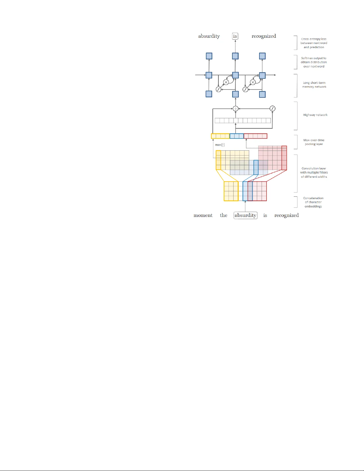
Character -A war e Neural Language Models Y oon Kim † † School of Engineering and Applied Sciences Harvard Uni versity { yoonkim,srush } @seas.harvard.edu Y acine Jer nite ∗ Da vid Sontag ∗ ∗ Courant Institute of Mathematical Sciences New Y ork Uni versity { jernite,dsontag } @cs.nyu.edu Alexander M. Rush † Abstract W e describe a simple neural language model that re- lies only on character-le vel inputs. Predictions are still made at the word-le vel. Our model employs a con- volutional neural network (CNN) and a highway net- work ov er characters, whose output is giv en to a long short-term memory (LSTM) recurrent neural net- work language model (RNN-LM). On the English Penn T reebank the model is on par with the existing state-of-the-art despite having 60% fewer parameters. On languages with rich morphology (Arabic, Czech, French, German, Spanish, Russian), the model out- performs word-le vel/morpheme-lev el LSTM baselines, again with fewer parameters. The results suggest that on many languages, character inputs are suf ficient for lan- guage modeling. Analysis of word representations ob- tained from the character composition part of the model rev eals that the model is able to encode, from characters only , both semantic and orthographic information. Introduction Language modeling is a fundamental task in artificial intel- ligence and natural language processing (NLP), with appli- cations in speech recognition, text generation, and machine translation. A language model is formalized as a probability distribution ov er a sequence of strings (words), and tradi- tional methods usually in volv e making an n -th order Marko v assumption and estimating n -gram probabilities via count- ing and subsequent smoothing (Chen and Goodman 1998). The count-based models are simple to train, but probabilities of rare n -grams can be poorly estimated due to data sparsity (despite smoothing techniques). Neural Language Models (NLM) address the n -gram data sparsity issue through parameterization of words as vectors (word embeddings) and using them as inputs to a neural net- work (Bengio, Ducharme, and V incent 2003; Mikolov et al. 2010). The parameters are learned as part of the training process. W ord embeddings obtained through NLMs exhibit the property whereby semantically close words are likewise close in the induced v ector space (as is the case with non- neural techniques such as Latent Semantic Analysis (Deer- wester , Dumais, and Harshman 1990)). Copyright c  2016, Association for the Advancement of Artificial Intelligence (www .aaai.org). All rights reserv ed. While NLMs ha ve been sho wn to outperform count-based n -gram language models (Mikolov et al. 2011), the y are blind to subword information (e.g. morphemes). For exam- ple, they do not know , a priori, that eventful , eventfully , un- eventful , and uneventfully should ha ve structurally related embeddings in the vector space. Embeddings of rare words can thus be poorly estimated, leading to high perplexities for rare words (and words surrounding them). This is espe- cially problematic in morphologically rich languages with long-tailed frequency distributions or domains with dynamic vocab ularies (e.g. social media). In this work, we propose a language model that lev er- ages subword information through a character -level con- volutional neural network (CNN), whose output is used as an input to a recurrent neural network language model (RNN-LM). Unlike previous works that utilize subword in- formation via morphemes (Botha and Blunsom 2014; Lu- ong, Socher, and Manning 2013), our model does not require morphological tagging as a pre-processing step. And, unlike the recent line of work which combines input word embed- dings with features from a character -lev el model (dos Santos and Zadrozny 2014; dos Santos and Guimaraes 2015), our model does not utilize word embeddings at all in the input layer . Given that most of the parameters in NLMs are from the word embeddings, the proposed model has significantly fewer parameters than previous NLMs, making it attractiv e for applications where model size may be an issue (e.g. cell phones). T o summarize, our contributions are as follows: • on English, we achiev e results on par with the existing state-of-the-art on the Penn T reebank (PTB), despite ha v- ing approximately 60% fe wer parameters, and • on morphologically rich languages (Arabic, Czech, French, German, Spanish, and Russian), our model outperforms various baselines (Kneser -Ney , w ord- lev el/morpheme-lev el LSTM), again with fewer parame- ters. W e have released all the code for the models described in this paper . 1 1 https://github .com/yoonkim/lstm- char- cnn Model The architecture of our model, shown in Figure 1, is straight- forward. Whereas a con ventional NLM takes word embed- dings as inputs, our model instead takes the output from a single-layer character -level con volutional neural network with max-ov er-time pooling. For notation, we denote v ectors with bold lower -case (e.g. x t , b ), matrices with bold upper-case (e.g. W , U o ), scalars with italic lower -case (e.g. x, b ), and sets with cursiv e upper - case (e.g. V , C ) letters. For notational conv enience we as- sume that words and characters hav e already been con verted into indices. Recurrent Neural Network A recurrent neural network (RNN) is a type of neural net- work architecture particularly suited for modeling sequen- tial phenomena. At each time step t , an RNN takes the input vector x t ∈ R n and the hidden state vector h t − 1 ∈ R m and produces the next hidden state h t by applying the following recursiv e operation: h t = f ( Wx t + Uh t − 1 + b ) (1) Here W ∈ R m × n , U ∈ R m × m , b ∈ R m are parameters of an af fine transformation and f is an element-wise nonlin- earity . In theory the RNN can summarize all historical in- formation up to time t with the hidden state h t . In practice howe ver , learning long-range dependencies with a vanilla RNN is dif ficult due to vanishing/e xploding gradients (Ben- gio, Simard, and Frasconi 1994), which occurs as a result of the Jacobian’ s multiplicati vity with respect to time. Long short-term memory (LSTM) (Hochreiter and Schmidhuber 1997) addresses the problem of learning long range dependencies by augmenting the RNN with a memory cell vector c t ∈ R n at each time step. Concretely , one step of an LSTM takes as input x t , h t − 1 , c t − 1 and produces h t , c t via the following intermediate calculations: i t = σ ( W i x t + U i h t − 1 + b i ) f t = σ ( W f x t + U f h t − 1 + b f ) o t = σ ( W o x t + U o h t − 1 + b o ) g t = tanh ( W g x t + U g h t − 1 + b g ) c t = f t  c t − 1 + i t  g t h t = o t  tanh ( c t ) (2) Here σ ( · ) and tanh ( · ) are the element-wise sigmoid and hy- perbolic tangent functions,  is the element-wise multipli- cation operator , and i t , f t , o t are referred to as input , for- get , and output gates. At t = 1 , h 0 and c 0 are initialized to zero vectors. Parameters of the LSTM are W j , U j , b j for j ∈ { i, f , o, g } . Memory cells in the LSTM are additiv e with respect to time, alleviating the gradient vanishing problem. Gradient exploding is still an issue, though in practice simple opti- mization strategies (such as gradient clipping) work well. LSTMs have been shown to outperform vanilla RNNs on many tasks, including on language modeling (Sundermeyer , Schluter , and Ney 2012). It is easy to extend the RNN/LSTM to two (or more) layers by having another network whose Figure 1: Architecture of our language model applied to an exam- ple sentence. Best viewed in color . Here the model takes absur dity as the current input and combines it with the history (as represented by the hidden state) to predict the next word, is . First layer performs a lookup of character embeddings (of dimension four) and stacks them to form the matrix C k . Then con volution operations are ap- plied between C k and multiple filter matrices. Note that in the abov e example we have twelve filters—three filters of width two (blue), four filters of width three (yello w), and fiv e filters of width four (red). A max-over -time pooling operation is applied to obtain a fixed-dimensional representation of the word, which is given to the highway network. The highway network’ s output is used as the input to a multi-layer LSTM. Finally , an affine transformation fol- lowed by a softmax is applied ov er the hidden representation of the LSTM to obtain the distribution over the next w ord. Cross en- tropy loss between the (predicted) distribution over next word and the actual next word is minimized. Element-wise addition, multi- plication, and sigmoid operators are depicted in circles, and af fine transformations (plus nonlinearities where appropriate) are repre- sented by solid arrows. input at t is h t (from the first netw ork). Indeed, having mul- tiple layers is often crucial for obtaining competiti ve perfor - mance on various tasks (P ascanu et al. 2013). Recurrent Neural Network Language Model Let V be the fixed size vocab ulary of words. A language model specifies a distribution ov er w t +1 (whose support is V ) given the historical sequence w 1: t = [ w 1 , . . . , w t ] . A re- current neural network language model (RNN-LM) does this by applying an af fine transformation to the hidden layer fol- lowed by a softmax: Pr ( w t +1 = j | w 1: t ) = exp ( h t · p j + q j ) P j 0 ∈V exp ( h t · p j 0 + q j 0 ) (3) where p j is the j -th column of P ∈ R m ×|V | (also referred to as the output embedding ), 2 and q j is a bias term. Similarly , for a con ventional RNN-LM which usually takes words as inputs, if w t = k , then the input to the RNN-LM at t is the input embedding x k , the k -th column of the embedding matrix X ∈ R n ×|V | . Our model simply replaces the input embeddings X with the output from a character-le vel con- volutional neural netw ork, to be described below . If we denote w 1: T = [ w 1 , · · · , w T ] to be the sequence of words in the training corpus, training in volv es minimizing the negati ve log-likelihood ( N LL ) of the sequence N LL = − T X t =1 log Pr ( w t | w 1: t − 1 ) (4) which is typically done by truncated backpropagation through time (W erbos 1990; Graves 2013). Character -level Con volutional Neural Network In our model, the input at time t is an output from a character-le vel con volutional neural network (CharCNN), which we describe in this section. CNNs (LeCun et al. 1989) hav e achiev ed state-of-the-art results on computer vi- sion (Krizhevsky , Sutske ver , and Hinton 2012) and ha ve also been sho wn to be ef fective for v arious NLP tasks (Collobert et al. 2011). Architectures employed for NLP applications differ in that the y typically in volve temporal rather than spa- tial con volutions. Let C be the vocabulary of characters, d be the dimen- sionality of character embeddings, 3 and Q ∈ R d ×|C | be the matrix character embeddings. Suppose that word k ∈ V is made up of a sequence of characters [ c 1 , . . . , c l ] , where l is the length of word k . Then the character-le vel representation of k is given by the matrix C k ∈ R d × l , where the j -th col- umn corresponds to the character embedding for c j (i.e. the c j -th column of Q ). 4 W e apply a narrow con volution between C k and a filter (or kernel ) H ∈ R d × w of width w , after which we add a bias and apply a nonlinearity to obtain a featur e map f k ∈ R l − w +1 . Specifically , the i -th element of f k is giv en by: f k [ i ] = tanh ( h C k [ ∗ , i : i + w − 1] , H i + b ) (5) 2 In our work, predictions are at the word-le vel, and hence we still utilize word embeddings in the output layer . 3 Giv en that |C | is usually small, some authors work with one- hot representations of characters. Ho wev er we found that using lower dimensional representations of characters (i.e. d < |C | ) per- formed slightly better . 4 T w o technical details warrant mention here: (1) we append start-of-word and end-of-word characters to each word to better represent prefixes and suffixes and hence C k actually has l + 2 columns; (2) for batch processing, we zero-pad C k so that the num- ber of columns is constant (equal to the max word length) for all words in V . where C k [ ∗ , i : i + w − 1] is the i -to- ( i + w − 1) -th column of C k and h A , B i = T r( AB T ) is the Frobenius inner product. Finally , we take the max-o ver-time y k = max i f k [ i ] (6) as the feature corresponding to the filter H (when applied to word k ). The idea is to capture the most important feature— the one with the highest value—for a giv en filter . A filter is essentially picking out a character n -gram, where the size of the n -gram corresponds to the filter width. W e hav e described the process by which one feature is obtained from one filter matrix. Our CharCNN uses multiple filters of v arying widths to obtain the feature vector for k . So if we have a total of h filters H 1 , . . . , H h , then y k = [ y k 1 , . . . , y k h ] is the input representation of k . For many NLP applications h is typically chosen to be in [100 , 1000] . Highway Network W e could simply replace x k (the word embedding) with y k at each t in the RNN-LM, and as we show later , this simple model performs well on its own (T able 7). One could also hav e a multilayer perceptron (MLP) ov er y k to model in- teractions between the character n -grams picked up by the filters, b ut we found that this resulted in worse performance. Instead we obtained improvements by running y k through a highway network , recently proposed by Sri vasta va et al. (2015). Whereas one layer of an MLP applies an affine trans- formation followed by a nonlinearity to obtain a ne w set of features, z = g ( Wy + b ) (7) one layer of a highway network does the follo wing: z = t  g ( W H y + b H ) + ( 1 − t )  y (8) where g is a nonlinearity , t = σ ( W T y + b T ) is called the transform gate, and ( 1 − t ) is called the carry gate. Similar to the memory cells in LSTM networks, highway layers allow for training of deep networks by adaptiv ely carrying some dimensions of the input directly to the output. 5 By construc- tion the dimensions of y and z have to match, and hence W T and W H are square matrices. Experimental Setup As is standard in language modeling, we use perplexity ( P P L ) to ev aluate the performance of our models. Perplex- ity of a model ov er a sequence [ w 1 , . . . , w T ] is gi ven by P P L = exp  N LL T  (9) where N LL is calculated over the test set. W e test the model on corpora of varying languages and sizes (statistics avail- able in T able 1). W e conduct hyperparameter search, model introspection, and ablation studies on the English Penn T reebank (PTB) (Marcus, Santorini, and Marcinkie wicz 1993), utilizing the 5 Sriv astav a et al. (2015) recommend initializing b T to a neg- ativ e value, in order to militate the initial behavior tow ards carry . W e initialized b T to a small interval around − 2 . D A TA - S D A TA - L |V | |C | T |V | |C | T English (E N ) 10 k 51 1 m 60 k 197 20 m Czech (C S ) 46 k 101 1 m 206 k 195 17 m German (D E ) 37 k 74 1 m 339 k 260 51 m Spanish (E S ) 27 k 72 1 m 152 k 222 56 m French (F R ) 25 k 76 1 m 137 k 225 57 m Russian (R U ) 62 k 62 1 m 497 k 111 25 m Arabic (A R ) 86 k 132 4 m – – – T able 1: Corpus statistics. |V | = word vocabulary size; |C | = char- acter vocabulary size; T = number of tokens in training set. The small English data is from the Penn Treebank and the Arabic data is from the News-Commentary corpus. The rest are from the 2013 A CL W orkshop on Machine Translation. |C | is large because of (rarely occurring) special characters. standard training (0-20), v alidation (21-22), and test (23-24) splits along with pre-processing by Mikolov et al. (2010). W ith approximately 1 m tokens and |V | = 10 k, this version has been extensi vely used by the language modeling com- munity and is publicly av ailable. 6 W ith the optimal hyperparameters tuned on PTB, we ap- ply the model to various morphologically rich languages: Czech, German, French, Spanish, Russian, and Arabic. Non- Arabic data comes from the 2013 A CL W orkshop on Ma- chine T ranslation, 7 and we use the same train/v alidation/test splits as in Botha and Blunsom (2014). While the raw data are publicly available, we obtained the preprocessed ver- sions from the authors, 8 whose morphological NLM serves as a baseline for our work. W e train on both the small datasets (D A TA - S ) with 1 m tokens per language, and the large datasets ( D AT A - L ) including the large English data which has a much bigger |V | than the PTB. Arabic data comes from the News-Commentary corpus, 9 and we per - form our own preprocessing and train/v alidation/test splits. In these datasets only singleton words were replaced with < unk > and hence we effecti vely use the full vocabulary . It is worth noting that the character model can utilize surface forms of OO V tokens (which were replaced with < unk > ), but we do not do this and stick to the preprocessed versions (de- spite disadvantaging the character models) for exact com- parison against prior work. Optimization The models are trained by truncated backpropagation through time (W erbos 1990; Graves 2013). W e backprop- agate for 35 time steps using stochastic gradient descent where the learning rate is initially set to 1 . 0 and halved if the perplexity does not decrease by more than 1 . 0 on the validation set after an epoch. On D AT A - S we use a batch size of 20 and on D A T A - L we use a batch size of 100 (for 6 http://www .fit.vutbr .cz/ ∼ imikolov/rnnlm/ 7 http://www .statmt.org/wmt13/translation- task.html 8 http://bothameister .github .io/ 9 http://opus.lingfil.uu.se/News- Commentary .php Small Large CNN d 15 15 w [1 , 2 , 3 , 4 , 5 , 6] [1 , 2 , 3 , 4 , 5 , 6 , 7] h [25 · w ] [ min { 200 , 50 · w } ] f tanh tanh Highway l 1 2 g ReLU ReLU LSTM l 2 2 m 300 650 T able 2: Architecture of the small and large models. d = dimensionality of character embeddings; w = filter widths; h = number of filter matrices, as a function of filter width (so the large model has filters of width [1 , 2 , 3 , 4 , 5 , 6 , 7] of size [50 , 100 , 150 , 200 , 200 , 200 , 200] for a total of 1100 filters); f , g = nonlinearity functions; l = number of layers; m = number of hidden units. greater efficiency). Gradients are averaged over each batch. W e train for 25 epochs on non-Arabic and 30 epochs on Ara- bic data (which was sufficient for con vergence), picking the best performing model on the validation set. Parameters of the model are randomly initialized over a uniform distribu- tion with support [ − 0 . 05 , 0 . 05] . For regularization we use dropout (Hinton et al. 2012) with probability 0 . 5 on the LSTM input-to-hidden layers (except on the initial Highway to LSTM layer) and the hidden-to-output softmax layer . W e further constrain the norm of the gradients to be below 5 , so that if the L 2 norm of the gradient exceeds 5 then we renormalize it to hav e || · || = 5 before updating. The gradient norm constraint was crucial in training the model. These choices were largely guided by previous work of Zaremba et al. (2014) on word- lev el language modeling with LSTMs. Finally , in order to speed up training on D AT A - L we em- ploy a hierarchical softmax (Morin and Bengio 2005)—a common strategy for training language models with very large |V | —instead of the usual softmax. W e pick the number of clusters c = d p |V |e and randomly split V into mutually exclusi ve and collectiv ely exhaustiv e subsets V 1 , . . . , V c of (approximately) equal size. 10 Then Pr ( w t +1 = j | w 1: t ) be- comes, Pr ( w t +1 = j | w 1: t ) = exp ( h t · s r + t r ) P c r 0 =1 exp ( h t · s r 0 + t r 0 ) × exp ( h t · p j r + q j r ) P j 0 ∈V r exp ( h t · p j 0 r + q j 0 r ) (10) where r is the cluster index such that j ∈ V r . The first term is simply the probability of picking cluster r , and the second 10 While Bro wn clustering/frequency-based clustering is com- monly used in the literature (e.g. Botha and Blunsom (2014) use Brown clusering), we used random clusters as our implementation enjoys the best speed-up when the number of words in each clus- ter is approximately equal. W e found random clustering to work surprisingly well. P P L Size LSTM-W ord-Small 97 . 6 5 m LSTM-Char-Small 92 . 3 5 m LSTM-W ord-Large 85 . 4 20 m LSTM-Char-Lar ge 78 . 9 19 m KN- 5 (Mik olov et al. 2012) 141 . 2 2 m RNN † (Mikolov et al. 2012) 124 . 7 6 m RNN-LD A † (Mikolov et al. 2012) 113 . 7 7 m genCNN † (W ang et al. 2015) 116 . 4 8 m FOFE-FNNLM † (Zhang et al. 2015) 108 . 0 6 m Deep RNN (Pascanu et al. 2013) 107 . 5 6 m Sum-Prod Net † (Cheng et al. 2014) 100 . 0 5 m LSTM-1 † (Zaremba et al. 2014) 82 . 7 20 m LSTM-2 † (Zaremba et al. 2014) 78 . 4 52 m T able 3: Performance of our model versus other neural language models on the English Penn Treebank test set. P P L refers to per- plexity (lower is better) and size refers to the approximate number of parameters in the model. KN- 5 is a Kneser-Ney 5 -gram language model which serves as a non-neural baseline. † For these models the authors did not explicitly state the number of parameters, and hence sizes sho wn here are estimates based on our understanding of their papers or priv ate correspondence with the respectiv e authors. term is the probability of picking word j giv en that cluster r is picked. W e found that hierarchical softmax was not nec- essary for models trained on D A TA - S . Results English Penn T reebank W e train two versions of our model to assess the trade-off between performance and size. Architecture of the small (LSTM-Char-Small) and large (LSTM-Char-Large) models is summarized in T able 2. As another baseline, we also train two comparable LSTM models that use word em- beddings only (LSTM-W ord-Small, LSTM-W ord-Large). LSTM-W ord-Small uses 200 hidden units and LSTM-W ord- Large uses 650 hidden units. W ord embedding sizes are also 200 and 650 respecti vely . These were chosen to keep the number of parameters similar to the corresponding character-le vel model. As can be seen from T able 3, our large model is on par with the existing state-of-the-art (Zaremba et al. 2014), despite ha ving approximately 60% fewer parameters. Our small model significantly outperforms other NLMs of sim- ilar size, even though it is penalized by the fact that the dataset already has OO V words replaced with < unk > (other models are purely word-le vel models). While lower perplex- ities have been reported with model ensembles (Mikolov and Zweig 2012), we do not include them here as they are not comparable to the current work. Other Languages The model’ s performance on the English PTB is informative to the extent that it facilitates comparison against the large body of existing work. Howe ver , English is relati vely simple D A TA - S C S D E E S F R R U A R Botha KN- 4 545 366 241 274 396 323 MLBL 465 296 200 225 304 – Small W ord 503 305 212 229 352 216 Morph 414 278 197 216 290 230 Char 401 260 182 189 278 196 Large W ord 493 286 200 222 357 172 Morph 398 263 177 196 271 148 Char 371 239 165 184 261 148 T able 4: T est set perple xities for D AT A - S . First two ro ws are from Botha (2014) (except on Arabic where we trained our own KN- 4 model) while the last six are from this paper . KN- 4 is a Kneser- Ney 4 -gram language model, and MLBL is the best performing morphological logbilinear model from Botha (2014). Small/Large refer to model size (see T able 2), and W ord/Morph/Char are models with words/morphemes/characters as inputs respecti vely . from a morphological standpoint, and thus our next set of results (and ar guably the main contribution of this paper) is focused on languages with richer morphology (T able 4, T able 5). W e compare our results against the morphological log- bilinear (MLBL) model from Botha and Blunsom (2014), whose model also takes into account subword information through morpheme embeddings that are summed at the input and output layers. As comparison against the MLBL mod- els is confounded by our use of LSTMs—widely kno wn to outperform their feed-forward/log-bilinear cousins—we also train an LSTM version of the morphological NLM, where the input representation of a w ord gi ven to the LSTM is a summation of the word’ s morpheme embeddings. Con- cretely , suppose that M is the set of morphemes in a lan- guage, M ∈ R n ×|M| is the matrix of morpheme embed- dings, and m j is the j -th column of M (i.e. a morpheme embedding). Given the input word k , we feed the following representation to the LSTM: x k + X j ∈M k m j (11) where x k is the word embedding (as in a word-le vel model) and M k ⊂ M is the set of morphemes for word k . The morphemes are obtained by running an unsupervised mor- phological tagger as a preprocessing step. 11 W e emphasize that the word embedding itself (i.e. x k ) is added on top of the morpheme embeddings, as was done in Botha and Blunsom (2014). The morpheme embeddings are of size 200 / 650 for the small/large models respectiv ely . W e further train word- lev el LSTM models as another baseline. On D A TA - S it is clear from T able 4 that the character- lev el models outperform their word-le vel counterparts de- 11 W e use Morfessor Cat-MAP (Creutz and Lagus 2007), as in Botha and Blunsom (2014). D A TA - L C S D E E S F R R U E N Botha KN- 4 862 463 219 243 390 291 MLBL 643 404 203 227 300 273 Small W ord 701 347 186 202 353 236 Morph 615 331 189 209 331 233 Char 578 305 169 190 313 216 T able 5: T est set perplexities on D AT A - L . First two rows are from Botha (2014), while the last three rows are from the small LSTM models described in the paper . KN- 4 is a Kneser-Ney 4 -gram lan- guage model, and MLBL is the best performing morphological log- bilinear model from Botha (2014). W ord/Morph/Char are models with words/morphemes/characters as inputs respecti vely . spite, again, being smaller . 12 The character models also out- perform their morphological counterparts (both MLBL and LSTM architectures), although improv ements over the mor - phological LSTMs are more measured. Note that the mor- pheme models have strictly more parameters than the word models because w ord embeddings are used as part of the in- put. Due to memory constraints 13 we only train the small models on D AT A - L (T able 5). Interestingly we do not ob- serve significant differences going from word to morpheme LSTMs on Spanish, French, and English. The character models again outperform the word/morpheme models. W e also observe significant perplexity reductions ev en on En- glish when V is large. W e conclude this section by noting that we used the same architecture for all languages and did not perform any language-specific tuning of hyperparame- ters. Discussion Learned W ord Representations W e explore the word representations learned by the models on the PTB. T able 6 has the nearest neighbors of word rep- resentations learned from both the word-le vel and character- lev el models. For the character models we compare the rep- resentations obtained before and after highway layers. Before the highway layers the representations seem to solely rely on surface forms—for example the nearest neigh- bors of you are your , young, four , youth , which are close to you in terms of edit distance. The highway layers howe ver , seem to enable encoding of semantic features that are not discernable from orthography alone. After highway layers the nearest neighbor of you is we , which is orthographically distinct from you . Another example is while and though — these w ords are far apart edit distance-wise yet the composi- tion model is able to place them near each other . The model 12 The difference in parameters is greater for non-PTB corpora as the size of the word model scales faster with |V | . For e xample, on Arabic the small/large word models ha ve 35 m/ 121 m parameters while the corresponding character models ha ve 29 m/ 69 m parame- ters respectiv ely . 13 All models were trained on GPUs with 2GB memory . Figure 2: Plot of character n -gram representations via PCA for English. Colors correspond to: prefixes (red), suffix es (blue), hy- phenated (orange), and all others (grey). Prefix es refer to character n -grams which start with the start-of-word character . Suffix es like- wise refer to character n -grams which end with the end-of-word character . also makes some clear mistakes (e.g. his and hhs ), highlight- ing the limits of our approach, although this could be due to the small dataset. The learned representations of OO V words ( computer- aided , misinformed ) are positioned near words with the same part-of-speech. The model is also able to correct for incorrect/non-standard spelling ( looooook ), indicating po- tential applications for text normalization in noisy domains. Learned Character N -gram Representations As discussed previously , each filter of the CharCNN is es- sentially learning to detect particular character n -grams. Our initial e xpectation was that each filter would learn to activ ate on different morphemes and then build up semantic repre- sentations of words from the identified morphemes. Ho w- ev er , upon re viewing the character n -grams picked up by the filters (i.e. those that maximized the value of the filter), we found that they did not (in general) correspond to valid morphemes. T o get a better intuition for what the character composi- tion model is learning, we plot the learned representations of all character n -grams (that occurred as part of at least two words in V ) via principal components analysis (Figure 2). W e feed each character n -gram into the CharCNN and use the CharCNN’ s output as the fixed dimensional representa- tion for the corresponding character n -gram. As is appar - ent from Figure 2, the model learns to differentiate between prefixes (red), suf fixes (blue), and others (grey). W e also find that the representations are particularly sensitiv e to character n -grams containing hyphens (orange), presumably because this is a strong signal of a word’ s part-of-speech. Highway Layers W e quantitatively in vestigate the effect of highway network layers via ablation studies (T able 7). W e train a model with- out any highway layers, and find that performance decreases significantly . As the difference in performance could be due to the decrease in model size, we also train a model that feeds y k (i.e. word representation from the CharCNN) In V ocabulary Out-of-V ocabulary while his you richar d trading computer -aided misinformed looooook LSTM-W ord although your conservatives jonathan advertised – – – letting her we r obert advertising – – – though my guys neil turnover – – – minute their i nancy turnover – – – chile this your har d heading computer-guided informed look LSTM-Char whole hhs young rich training computerized performed cook (before highway) meanwhile is four richer r eading disk-drive transformed looks white has youth richter leading computer inform shook meanwhile hhs we eduard tr ade computer-guided informed look LSTM-Char whole this your ger ar d training computer-driven performed looks (after highway) though their doug edwar d traded computerized outperformed looked nevertheless your i carl trader computer transformed looking T able 6: Nearest neighbor words (based on cosine similarity) of word representations from the lar ge word-lev el and character -lev el (before and after highway layers) models trained on the PTB. Last three words are OO V words, and therefore the y do not have representations in the word-le vel model. LSTM-Char Small Large No Highway Layers 100 . 3 84 . 6 One Highway Layer 92 . 3 79 . 7 T wo Highway Layers 90 . 1 78 . 9 One MLP Layer 111 . 2 92 . 6 T able 7: Perplexity on the Penn Treebank for small/large models trained with/without highway layers. through a one-layer multilayer perceptron (MLP) to use as input into the LSTM. W e find that the MLP does poorly , al- though this could be due to optimization issues. W e hypothesize that highway networks are especially well-suited to work with CNNs, adapti vely combining lo- cal features detected by the individual filters. CNNs hav e already prov en to be been successful for many NLP tasks (Collobert et al. 2011; Shen et al. 2014; Kalchbrenner , Grefenstette, and Blunsom 2014; Kim 2014; Zhang, Zhao, and LeCun 2015; Lei, Barzilay , and Jaakola 2015), and we posit that further gains could be achieved by employing highway layers on top of existing CNN architectures. W e also anecdotally note that (1) having one to two high- way layers was important, but more highway layers gener- ally resulted in similar performance (though this may de- pend on the size of the datasets), (2) having more conv olu- tional layers before max-pooling did not help, and (3) high- way layers did not improv e models that only used w ord em- beddings as inputs. Effect of Corpus/V ocab Sizes W e next study the effect of training corpus/vocab ulary sizes on the relative performance between the different models. W e take the German (D E ) dataset from D A T A - L and v ary the training corpus/vocab ulary sizes, calculating the perplex- |V | 10 k 25 k 50 k 100 k T 1 m 17% 16% 21% – 5 m 8% 14% 16% 21% 10 m 9% 9% 12% 15% 25 m 9% 8% 9% 10% T able 8: Perplexity reductions by going from small word-le vel to character-le vel models based on different corpus/vocab ulary sizes on German ( D E ). |V | is the vocab ulary size and T is the number of tokens in the training set. The full vocab ulary of the 1 m dataset was less than 100 k and hence that scenario is una vailable. ity reductions as a result of going from a small word-le vel model to a small character -le vel model. T o vary the vocab u- lary size we take the most frequent k words and replace the rest with < unk > . As with pre vious experiments the character model does not utilize surface forms of < unk > and simply treats it as another token. Although T able 8 suggests that the perplexity reductions become less pronounced as the corpus size increases, we nonetheless find that the character-le vel model outperforms the word-le vel model in all scenarios. Further Observations W e report on some further experiments and observations: • Combining word embeddings with the CharCNN’ s out- put to form a combined representation of a word (to be used as input to the LSTM) resulted in slightly worse performance ( 81 on PTB with a large model). This was surprising, as improvements hav e been reported on part- of-speech tagging (dos Santos and Zadrozny 2014) and named entity recognition (dos Santos and Guimaraes 2015) by concatenating word embeddings with the out- put from a character-le vel CNN. While this could be due to insufficient experimentation on our part, 14 it suggests that for some tasks, word embeddings are superfluous— character inputs are good enough. • While our model requires additional con volution opera- tions ov er characters and is thus slo wer than a comparable word-le vel model which can perform a simple lookup at the input layer , we found that the dif ference was manage- able with optimized GPU implementations—for example on PTB the lar ge character -lev el model trained at 1500 to- kens/sec compared to the word-le vel model which trained at 3000 tokens/sec. For scoring, our model can ha ve the same running time as a pure word-le vel model, as the CharCNN’ s outputs can be pre-computed for all words in V . This would, howe ver , be at the expense of increased model size, and thus a trade-of f can be made between run-time speed and memory (e.g. one could restrict the pre-computation to the most frequent words). Related W ork Neural Language Models (NLM) encompass a rich fam- ily of neural network architectures for language modeling. Some example architectures include feed-forward (Bengio, Ducharme, and V incent 2003), recurrent (Mikolov et al. 2010), sum-product (Cheng et al. 2014), log-bilinear (Mnih and Hinton 2007), and con volutional (W ang et al. 2015) net- works. In order to address the rare word problem, Alexandrescu and Kirchhoff (2006)—b uilding on analogous work on count-based n -gram language models by Bilmes and Kirch- hoff (2003)—represent a word as a set of shared factor em- beddings. Their Factored Neural Language Model (FNLM) can incorporate morphemes, word shape information (e.g. capitalization) or an y other annotation (e.g. part-of-speech tags) to represent words. A specific class of FNLMs le verages morphemic infor- mation by vie wing a word as a function of its (learned) morpheme embeddings (Luong, Socher , and Manning 2013; Botha and Blunsom 2014; Qui et al. 2014). For example Lu- ong, Socher , and Manning (2013) apply a recursiv e neural network over morpheme embeddings to obtain the embed- ding for a single word. While such models ha ve prov ed use- ful, they require morphological tagging as a preprocessing step. Another direction of work has in volved purely character- lev el NLMs, wherein both input and output are charac- ters (Sutskev er, Martens, and Hinton 2011; Grav es 2013). Character-le vel models obviate the need for morphological tagging or manual feature engineering, and hav e the attrac- tiv e property of being able to generate nov el words. How- ev er they are generally outperformed by word-le vel models (Mikolov et al. 2012). Outside of language modeling, improvements have been reported on part-of-speech tagging (dos Santos and Zadrozny 2014) and named entity recognition (dos Santos 14 W e experimented with (1) concatenation, (2) tensor products, (3) averaging, and (4) adapti ve weighting schemes whereby the model learns a con vex combination of word embeddings and the CharCNN outputs. and Guimaraes 2015) by representing a word as a concatena- tion of its word embedding and an output from a character- lev el CNN, and using the combined representation as fea- tures in a Conditional Random Field (CRF). Zhang, Zhao, and LeCun (2015) do aw ay with word embeddings com- pletely and show that for text classification, a deep CNN ov er characters performs well. Ballesteros, Dyer, and Smith (2015) use an RNN over characters only to train a transition- based parser, obtaining improvements on many morpholog- ically rich languages. Finally , Ling et al. (2015) apply a bi-directional LSTM ov er characters to use as inputs for language modeling and part-of-speech tagging. The y sho w improv ements on various languages (English, Portuguese, Catalan, German, T urkish). It remains open as to which character composition model (i.e. CNN or LSTM) performs better . Conclusion W e hav e introduced a neural language model that utilizes only character-le vel inputs. Predictions are still made at the word-le vel. Despite having fe wer parameters, our model outperforms baseline models that utilize word/morpheme embeddings in the input layer . Our work questions the ne- cessity of word embeddings (as inputs) for neural language modeling. Analysis of word representations obtained from the char- acter composition part of the model further indicates that the model is able to encode, from characters only , rich se- mantic and orthographic features. Using the CharCNN and highway layers for representation learning (e.g. as input into word2v ec (Mikolov et al. 2013)) remains an avenue for fu- ture work. Insofar as sequential processing of words as inputs is ubiquitous in natural language processing, it would be in- teresting to see if the architecture introduced in this paper is viable for other tasks—for example, as an encoder/decoder in neural machine translation (Cho et al. 2014; Sutskev er, V inyals, and Le 2014). Acknowledgments W e are especially grateful to Jan Botha for providing the preprocessed datasets and the model results. References Alexandrescu, A., and Kirchhoff, K. 2006. Factored Neural Lan- guage Models. In Pr oceedings of NAA CL . Ballesteros, M.; Dyer , C.; and Smith, N. A. 2015. Im- prov ed Transition-Based Parsing by Modeling Characters instead of Words with LSTMs. In Pr oceedings of EMNLP . Bengio, Y .; Ducharme, R.; and V incent, P . 2003. A Neural Prob- abilistic Language Model. Journal of Machine Learning Resear ch 3:1137–1155. Bengio, Y .; Simard, P .; and Frasconi, P . 1994. Learning Long-term Dependencies with Gradient Descent is Difficult. IEEE T ransac- tions on Neural Networks 5:157–166. Bilmes, J., and Kirchhoff, K. 2003. Factored Language Models and Generalized Parallel Backof f. In Proceedings of N AACL . Botha, J., and Blunsom, P . 2014. Compositional Morphology for Word Representations and Language Modelling. In Pr oceedings of ICML . Botha, J. 2014. Probabilistic Modelling of Morphologically Rich Languages. DPhil Dissertation, Oxfor d University . Chen, S., and Goodman, J. 1998. An Empirical Study of Smooth- ing T echniques for Language Modeling. T echnical Report, Har- var d University . Cheng, W . C.; K ok, S.; Pham, H. V .; Chieu, H. L.; and Chai, K. M. 2014. Language Modeling with Sum-Product Networks. In Pro- ceedings of INTERSPEECH . Cho, K.; van Merrienboer, B.; Gulcehre, C.; Bahdanau, D.; Bougares, F .; Schwenk, H.; and Bengio, Y . 2014. Learning Phrase Representations using RNN Encoder-Decoder for Statistical Ma- chine T ranslation. In Proceedings of EMNLP . Collobert, R.; W eston, J.; Bottou, L.; Karlen, M.; Kavukcuoglu, K.; and Kuksa, P . 2011. Natural Language Processing (almost) from Scratch. Journal of Mac hine Learning Researc h 12:2493–2537. Creutz, M., and Lagus, K. 2007. Unsupervised Models for Mor- pheme Segmentation and Morphology Learning. In Proceedings of the A CM T ransations on Speech and Langua ge Pr ocessing . Deerwester , S.; Dumais, S.; and Harshman, R. 1990. Indexing by Latent Semantic Analysis. Journal of American Society of Infor- mation Science 41:391–407. dos Santos, C. N., and Guimaraes, V . 2015. Boosting Named Entity Recognition with Neural Character Embeddings. In Proceedings of A CL Named Entities W orkshop . dos Santos, C. N., and Zadrozny , B. 2014. Learning Character- lev el Representations for Part-of-Speech Tagging. In Pr oceedings of ICML . Grav es, A. 2013. Generating Sequences with Recurrent Neural Networks. . Hinton, G.; Sri vasta va, N.; Krizhevsky , A.; Sutske ver , I.; and Salakhutdinov , R. 2012. Improving Neural Networks by Prevent- ing Co-Adaptation of Feature Detectors. . Hochreiter , S., and Schmidhuber , J. 1997. Long Short-Term Mem- ory . Neural Computation 9:1735–1780. Kalchbrenner , N.; Grefenstette, E.; and Blunsom, P . 2014. A Con- volutional Neural Network for Modelling Sentences. In Pr oceed- ings of A CL . Kim, Y . 2014. Con volutional Neural Networks for Sentence Clas- sification. In Pr oceedings of EMNLP . Krizhevsk y , A.; Sutske ver , I.; and Hinton, G. 2012. ImageNet Classification with Deep Con volutional Neural Networks. In Pr o- ceedings of NIPS . LeCun, Y .; Boser , B.; Denk er, J. S.; Henderson, D.; How ard, R. E.; Hubbard, W .; and Jackel, L. D. 1989. Handwritten Digit Recogni- tion with a Backpropagation Network. In Pr oceedings of NIPS . Lei, T .; Barzilay , R.; and Jaakola, T . 2015. Molding CNNs for Text: Non-linear , Non-consecutive Con volutions. In Pr oceedings of EMNLP . Ling, W .; Lui, T .; Marujo, L.; Astudillo, R. F .; Amir , S.; Dyer , C.; Black, A. W .; and Trancoso, I. 2015. Finding Function in Form: Compositional Character Models for Open V ocabulary Word Rep- resentation. In Pr oceedings of EMNLP . Luong, M.-T .; Socher , R.; and Manning, C. 2013. Better Word Representations with Recursiv e Neural Networks for Morphology . In Pr oceedings of CoNLL . Marcus, M.; Santorini, B.; and Marcinkiewicz, M. 1993. Building a Lar ge Annotated Corpus of English: the Penn T reebank. Compu- tational Linguistics 19:331–330. Mikolov , T ., and Zweig, G. 2012. Context Dependent Recurrent Neural Network Language Model. In Proceedings of SL T . Mikolov , T .; Karafiat, M.; Burget, L.; Cernock y , J.; and Khudanpur , S. 2010. Recurrent Neural Network Based Language Model. In Pr oceedings of INTERSPEECH . Mikolov , T .; Deoras, A.; Kombrink, S.; Burget, L.; and Cernocky , J. 2011. Empirical Evaluation and Combination of Advanced Lan- guage Modeling T echniques. In Proceedings of INTERSPEECH . Mikolov , T .; Sutske ver , I.; Deoras, A.; Le, H.-S.; Kombrink, S.; and Cernocky , J. 2012. Subword Language Modeling with Neural Networks. preprint: www .fit.vutbr .cz/ ˜ imikolov/rnnlm/c har .pdf . Mikolov , T .; Chen, K.; Corrado, G.; and Dean, J. 2013. Ef- ficient Estimation of Word Representations in V ector Space. arXiv:1301.3781 . Mnih, A., and Hinton, G. 2007. Three New Graphical Models for Statistical Language Modelling. In Pr oceedings of ICML . Morin, F ., and Bengio, Y . 2005. Hierarchical Probabilistic Neural Network Language Model. In Proceedings of AIST A TS . Pascanu, R.; Culcehre, C.; Cho, K.; and Bengio, Y . 2013. How to Construct Deep Neural Networks. . Qui, S.; Cui, Q.; Bian, J.; and Gao, B. 2014. Co-learning of Word Representations and Morpheme Representations. In Pr oceedings of COLING . Shen, Y .; He, X.; Gao, J.; Deng, L.; and Mesnil, G. 2014. A Latent Semantic Model with Conv olutional-pooling Structure for Infor- mation Retriev al. In Pr oceedings of CIKM . Sriv astav a, R. K.; Greff, K.; and Schmidhuber , J. 2015. Training Very Deep Networks. . Sundermeyer , M.; Schluter , R.; and Ney , H. 2012. LSTM Neural Networks for Language Modeling. Sutske ver , I.; Martens, J.; and Hinton, G. 2011. Generating Text with Recurrent Neural Networks. Sutske ver , I.; V inyals, O.; and Le, Q. 2014. Sequence to Sequence Learning with Neural Networks. W ang, M.; Lu, Z.; Li, H.; Jiang, W .; and Liu, Q. 2015. g en CNN: A Conv olutional Architecture for Word Sequence Prediction. In Pr oceedings of ACL . W erbos, P . 1990. Back-propagation Through Time: what it does and how to do it. In Pr oceedings of IEEE . Zaremba, W .; Sutskev er, I.; and V inyals, O. 2014. Recurrent Neural Network Regularization. . Zhang, S.; Jiang, H.; Xu, M.; Hou, J.; and Dai, L. 2015. The Fixed- Size Ordinally-Forgetting Encoding Method for Neural Network Language Models. In Pr oceedings of ACL . Zhang, X.; Zhao, J.; and LeCun, Y . 2015. Character -level Con vo- lutional Networks for Te xt Classification. In Pr oceedings of NIPS .