Efficient Nonnegative Tucker Decompositions: Algorithms and Uniqueness
Nonnegative Tucker decomposition (NTD) is a powerful tool for the extraction of nonnegative parts-based and physically meaningful latent components from high-dimensional tensor data while preserving the natural multilinear structure of data. However,…
Authors: Guoxu Zhou, Andrzej Cichocki, Qibin Zhao
IEEE TRANSA CTIONS ON IMA GE PR OCESSING 1 Ef ficient Nonne gati ve T ucker Decompositions: Algorithms and Uniqueness Guoxu Zhou, Andrzej Cichocki F ellow , IEEE , Qibin Zhao, and Shengli Xie Senior Member , IEEE, Abstract —Nonnegative T ucker decomposition (NTD) is a pow- erful tool for the extraction of nonnegati ve parts-based and physically meaningful latent components from high-dimensional tensor data while preser ving the natural multilinear structure of data. However , as the data tensor often has multiple modes and is large-scale, existing NTD algorithms suffer from a very high computational complexity in terms of both storage and computation time, which has been one major obstacle for practical applications of NTD. T o overcome these disadvantages, we show how low (multilinear) rank approximation (LRA) of tensors is able to significantly simplify the computation of the gradients of the cost function, upon which a family of efficient first-order NTD algorithms are developed. Besides dramatically reducing the storage complexity and running time, the new algorithms are quite flexible and robust to noise because any well-established LRA approaches can be applied. W e also show how nonnegativity incorporating sparsity substantially improves the uniqueness property and partially alleviates the curse of dimensionality of the T ucker decompositions. Simulation results on synthetic and real-world data justify the validity and high efficiency of the proposed NTD algorithms. Index T erms —T ucker decompositions, dimensionality reduc- tion, nonnegative alternating least squares. I . I N T R O D U C T I O N F INDING information-rich and task-relev ant variables hid- den behind observation data is a fundamental task in data analysis and has been widely studied in the fields of signal and image processing and machine learning. Although the observation data can be very large, a much lower num- ber of latent variables or components can capture the most significant features of the original data. By rev ealing such components, we achieve objectives such as dimensionality reduction and feature extraction and obtain a highly relev ant Manuscript received ...This work was partially supported by the National Natural Science Foundation of China (grants U1201253), the Guangdong Province Natural Science Foundation (2014A030308009), the Guangdong Province Excellent Thesis Foundation (SYBZZXM201316), and the JSPS KAKENHI (26730125, 15K15955). Guoxu Zhou is with the School of Automation at Guangdong University of T echnology , Guangzhou, China and the Laboratory for Advanced Brain Signal Processing, RIKEN Brain Science Institute, W ako-shi, Saitama, Japan. E-mail: zhouguoxu@ieee.org. Andrzej Cichocki is with the Laboratory for Advanced Brain Signal Processing, RIKEN Brain Science Institute, W ako-shi, Saitama, Japan and with Systems Research Institute, Polish Academy of Science, W arsaw , Poland. E-mail: cia@brain.riken.jp. Qibin Zhao is with the Laboratory for Advanced Brain Signal Processing, RIKEN Brain Science Institute, Japan. E-mail: qbzhao@brain.riken.jp. Shengli Xie is with the Faculty of Automation, Guangdong Univ ersity of T echnology , Guangzhou 510006, China. E-mail: eeoshlxie@scut.edu.cn. and compact representation of high-dimensional data. This important topic has been extensi vely studied in the last several decades, particularly witnessed by the great success of blind source separation (BSS) techniques [1]. In these methods, observation data are modeled as a linear combination of the latent components that possess specific div ersities such as statistical independence, a temporal structure, sparsity , and smoothness. By properly exploiting such diversities, a large family of matrix-factorization-based methodologies has been proposed and successfully applied to a v ariety of areas. In many applications, the data are more naturally represented by tensors, e.g., color images, video clips, and fMRI data. The methodologies that matricize the data and then apply matrix factorization approaches give a flattened view of data and often cause a loss of the internal structure information; hence, it is more fa vorable to process such data in their own domain, i.e., tensor domain, to obtain a multiple perspective stereoscopic view of data rather than a flattened one. For this reason, tensor decomposition methods have been proposed and widely applied to deal with high-order tensors. As one of the most widely used methods, the T ucker decomposition has been applied to pattern recognition [2], [3], clustering analysis [4], image denoising [5], etc. and has achieved great success. V ery often, the observation data and latent components are naturally nonnegati ve, e.g., text, images, spectra, probability matrices, the adjacency matrices of graphs, web data based on impressions and clicks, and financial time series. For these data, the extracted components may lose most of their physical meaning if the nonnegati vity is not preserved. In this regard, nonnegati ve matrix factorization (NMF) has been demonstrated to be a powerful tool to analyze nonnegativ e matrix data because NMF is able to gi ve physically meaningful and more interpretable results. Particularly , it has the ability of learning the local parts of objects [6]. As a result, NMF has receiv ed extensiv e study in the last decade [4], [6] and has been found many important applications including clus- tering analysis [7]–[9], sparse coding [10], dependent source separation [11], etc. For nonnegati ve tensor data analysis, nonnegati ve T ucker decomposition (NTD) has also gained importance in recent years [4], [12], [13]. NTD not only inherits all of the advan- tages of NMF but also provides an additional multiway struc- tured representation of data. Fig.1 illustrates how NTD is able to giv e a parts-based representation of face images included 2 IEEE TRANSA CTIONS ON IMA GE PR OCESSING A (1) ⊤ A (2) ! ⊤ !! G Weights: ≈ × 0.00 + × 0.08 + × 0.06 + × 0.14 + × 0.33 + × 0.08 + × 0.09 + × 0.11 + × 0.06 + × 0.05 Basis images Fig. 1: An illustration of how NTD is able to giv e a local parts-based representation of tensor objects for the PIE face database. By NTD, each face is represented by a linear combination of a set of very sparse basis faces. In contrast to the basis images extracted by NMF , these basis faces possess a multilinear structure (i.e., G × 1 A (1) × 2 A (2) ). T ABLE I: Notation and Definitions. A , a r , a ir A matrix, the r th-column, and the ( i, r )th-entry of matrix A , respectively . 1 , 0 The vector/matrix with all its elements being ones, zeros. I N The index set of positive integers no larger than N in ascending order, i.e., I N = { 1 , 2 , . . . , N } . R R 1 × R 2 ···× R N + Set of N th-order nonnegati ve tensors (matrices) with the size of R 1 -by- R 2 · · · by- R N . A ≥ 0 Nonnegati ve matrix A , i.e., a ir ≥ 0 , ∀ i, r . P + ( A ) An operator yielding a nonnegativ e matrix of a ir = max( a ir , 0) , ∀ i, r . Y , Y ( n ) A tensor, the mode- n matricization of tensor Y . ~ , Element-wise (Hadamard) product, division of matrices or tensors. Moreover , we define A B . = A B . C = A ⊗ B Kronecker product of A ∈ R I 1 × J 1 and B ∈ R I 2 × J 2 that yields C = [ a i 1 j 1 B ] ∈ R I 1 I 2 × J 1 J 2 with entries c ( i 1 − 1) I 2 + i 2 , ( j 1 − 1) J 2 + j 2 = a i 1 j 1 b i 2 j 2 . C = A B Khatri–Rao product of A = a 1 a 2 · · · a J ∈ R I 1 × J and B = b 1 b 2 · · · b J ∈ R I 2 × J that yields a matrix C = a 1 ⊗ b 1 a 2 ⊗ b 2 · · · a J ⊗ b J ∈ R I 1 I 2 × J . z A , s A Number of zeros in A ∈ R I × R , the sparsity defined as s A . = z A / ( I R ) ∈ [0 , 1] . A ∼ U (0 , 1) Elements of A are drawn from independent uniform distributions between 0 and 1. in the PIE database 1 . In the figure, a sample face image is represented as a linear combination of a set of sparse basis images that possess a multilinear structure. Unconstrained T ucker decompositions are often criticized for the lack of uniqueness and the curse of dimensionality , which indicates that the size of the core tensor increases exponentially with the dimension. Compared with unconstrained T ucker decomposi- tions, NTD is more likely to be unique and provides physically meaningful components. Moreov er , the core tensor in NTD is often v ery sparse, which allo ws us to discover the most significant links between components and to partially alle viate the curse of dimensionality . Unfortunately , existing algorithms are generally performed by directly applying the NMF update 1 A vailable at http://vasc.ri.cmu.edu/idb/html/face/. rules without fully exploiting the special multilinear structure of the T ucker model, which in turn suffers from a very high computational complexity in terms of both space and time, especially when the data tensor is large-scale. It is therefore quite crucial to develop more efficient NTD algorithms that are able to yield satisfactory results within a tolerable time. By taking into account that unconstrained Tuck er decompo- sitions are significantly faster than NTD, we propose a new framew ork for efficient NTD that is based on an unconstrained T ucker decomposition of the data tensor in this paper . As such, frequent access to the original big tensor is av oided, thereby leading to a considerably reduced computational complexity for NTD. Although the basic idea of NTD based on a proceeding low (multilinear) rank approximation (LRA) has been briefly introduced in our recent overvie w paper [14], the detailed deri vations are presented in this paper with new results on the uniqueness of NTD. The rest of the paper is organized as follows. In Section II, the basic notation and NTD models are introduced. In Section III, the first-order NTD algorithms are revie wed. In Section IV , flexible and efficient NTD algorithms based on the low-rank approximation of data are introduced, and unique and sparse NTD is discussed in Section V . Simulations on synthetic and real-world data are presented in Section VI to demonstrate the high ef ficiency of the proposed algorithms, and conclusions are presented in Section VII. The notation used in this paper is listed in T ABLE I, and more details can be found in [4], [15]. I I . N T D M O D E L S A. Notation and Basic Multilinear Operators Definitions. For an N th-order tensor G ∈ R R 1 × R 2 ···× R N , we define • Fibers. A mode- n fiber of tensor G is a vector ob- tained by fixing all indices but the n th index, e.g., g r 1 ,...,r n − 1 , : ,r n +1 ,...,r N , by using the MA TLAB colon op- erator . ZHOU et al. : EFFICIENT NONNEGA TIVE TUCKER DECOMPOSITIONS: ALGORITHMS AND UNIQUENESS 3 • Matricization. The mode- n matricization (unfolding) of G is an R n -by- Q p 6 = n R p matrix denoted by G ( n ) whose columns consist of all mode- n fibers of G . • Mode- n product. The mode- n product of G and an I n - by- R n matrix A ( n ) yields an N th-order tensor Y = G × n A ( n ) ∈ R R 1 ···× R n − 1 × I n × R n +1 ···× R N such that y r 1 , ··· ,r n − 1 ,i n ,r n +1 , ··· ,r N = R n X r n =1 g r 1 ,r 2 , ··· ,r N a i n ,r n . Useful properties. The following properties concerning the mode- n product will be frequently used: 1) If Y = G × n A ( n ) , then Y ( n ) = A ( n ) G ( n ) ; 2) ( G × n A ) × n B = G × n ( BA ) ; 3) ( G × m A ) × n B = ( G × n B ) × m A , n 6 = m . 4) If Y = G × 1 A (1) × 2 A (2) · · · × N A ( N ) . = G × n ∈I N A ( n ) , then Y ( n ) = A ( n ) G ( n ) R ( n ) > , where R ( n ) = A ( N ) ⊗ · · · ⊗ A ( n +1) ⊗ A ( n − 1) ⊗ · · · ⊗ A (1) . = O p 6 = n A ( p ) , (1) and Y ( n ) and G ( n ) are the mode- n matricizations of Y and G , respectiv ely . Note that owning to Property 3), the mode products in G × n ∈I N A ( n ) can be in any order of n . Howe ver , in N p 6 = n A ( p ) , the Kronecker products must be performed in the in verse order of the index set p 6 = n . = { 1 , 2 , . . . , n − 1 , n + 1 , . . . , N } . B. Nonnegative T uck er Decomposition Models 1) General NTD Model: By Tuck er decomposition, a given N th-order tensor Y ∈ R I 1 × I 2 ···× I N is approximated as Y ≈ G × n ∈I N A ( n ) , (2) where A ( n ) = h a ( n ) 1 a ( n ) 2 · · · a ( n ) R n i ∈ R I n × R n are the factor (component) matrices with rank ( A ( n ) ) = R n , and G ∈ R R 1 × R 2 ×···× R N is the core tensor whose entries reflect the interactions and connections between the components (columns) in different mode matrices. W e assume that R n ≤ I n as high-dimensional data can often be well approximated by its lower -rank representations. In NTD, both the core tensor G and the factor matrices A ( n ) are required to be element-wisely nonnegati ve. The nonnegati vity of the factors brings about two key effects: the resulting representation is purely additiv e but without subtractions, and the factors are often sparse, as they may contain man y zero entries. These two ef fects equip nonnegati ve factorization methods with the ability of learning localized parts of objects. 2) P opulation NTD: In the above NTD, if we fix the N th factor matrix A ( N ) to be the identity matrix I (or equiv alently , A ( N ) is absorbed into the core tensor such that G ← G × N A ( N ) [4]), we obtain the population NTD model: Y ≈ G × n 6 = N A ( n ) , A ( n ) ≥ 0 , G ≥ 0 . (3) Population NTD is important because it has a broad range of applications in machine learning and signal processing [4]. T o understand the key idea of population NTD, consider simultaneously performing NTD on a set of ( N − 1) th-order sample tensors { Y i ∈ R I 1 × I 2 ···× I N − 1 + : i = 1 , 2 , . . . , I N } with common component matrices. As such, each sample tensor can be represented as [4] Y i ≈ G i × n 6 = N A ( n ) , i = 1 , 2 , . . . , I N , (4) where G i is the core tensor associated with Y i , or equivalently , Y > ( N ) ≈ h O n 6 = N A ( n ) i G > ( N ) , (5) where each column of Y > ( N ) is a vectorized sample, and Y ( N ) is just the mode- N matricization of the N th-order tensor Y obtained by concatenating all of the samples Y i . As such, all samples are represented as a linear combination of N − 1 sets of common basis vectors (i.e., the columns of A ( n ) , n 6 = N ), and G i contains the extracted features. In the case of N = 3 , the tensors Y i and G i in (4) are just matrices, and (4) can be written as Y i ≈ A (1) G i A (2) > , (6) which has been studied in name of population value decom- position (PVD) [16] without nonnegati vity constraints. Hence, population NTD is an extension of PVD for extracting the nonnegati ve common components from multiblock higher- dimensional data equipped with the extra ability of learning the localized parts of objects [17]. An alternative method of performing such feature extraction tasks, which is referred to as nonnegati ve matrix factorization (NMF), vectorizes each sample to form a sample matrix S = Y > ( N ) = v ec ( Y 1 ) vec ( Y 2 ) · · · v ec ( Y I N ) . By using NMF , S is represented as S = Y > ( N ) ≈ WH > , s.t. W ≥ 0 , H ≥ 0 , (7) or equiv alently , by using tensor notation, S ≈ W × 2 H , s.t. W ≥ 0 , H ≥ 0 . (8) An intuitiv e difference between population NTD and NMF is that the basis vectors in the former are the outer product of lo wer-dimensional vectors, as shown in (5), which has a much lower number of free parameters and gi ves a kind of multilinear representation. This multilinear representation has been widely exploited to overcome the ov er-fitting problem in discriminant analysis [3], [18], and it substantially improves the sparsity of basis vectors, which will be discussed later . 4 IEEE TRANSA CTIONS ON IMA GE PR OCESSING I I I . O V E RV I E W O F F I R S T - O R D E R M E T H O D S F O R N T D In NTD, we need to minimize the following cost function: D NTD = 1 2 Y − b Y 2 F , (9) where b Y = G × n ∈I N A ( n ) with the component matrices A ( n ) ∈ R I n × R n + and the core tensor G ∈ R R 1 × R 2 ···× R N + , both of which are element-wisely nonnegati ve. Follo wing the analysis in [19] and similarly defining ∆ d = { x ∈ R d +1 + k k x k 1 = 1 } , we can straightforwardly obtain the following proposition: Proposition 1: Let Y ∈ R I 1 × I 2 ···× I N + . Then, the infimum inf n Y − G × n ∈I N A ( n ) 1 G ∈ R R 1 × R 2 ···× R N + , a ( n ) j ∈ ∆ R n − 1 , j ∈ I R n , n ∈ I N o is attained. Owning to Proposition 1 and the equiv alence of different norms, a global optimal solution for the problem in (9) always exists. Below , we focus on the optimization algorithms. T o solve the optimization problem, we generally use a block coordinate descent framew ork: we minimize the cost function with respect to only the partial parameters (e.g., one factor matrix or e ven only one column of it) each time while fixing the others. T o optimize A ( n ) , we consider an equi valent form of (9) by considering the mode- n matricization of Y and b Y : D NTD = 1 2 Y ( n ) − A ( n ) B ( n ) > 2 F , A ( n ) ≥ 0 , (10) where B ( n ) = R ( n ) G > ( n ) and R ( n ) is defined as in (1). T o optimize G , considering the v ectorization of Y and b Y , (9) becomes D NTD = 1 2 k vec ( Y ) − F vec ( G ) k 2 F , G ≥ 0 , (11) where F = O n ∈I N A ( n ) ∈ R ( Q n I n ) × ( Q n R n ) . (12) Both (10) and (11) are nonnegati ve least squares (NLS) problems and hav e been extensi vely studied in the context of NMF , including the multiplicative update (MU) algorithm [20], the hierarchical alternating least squares (HALS) method [4], the acti ve-set methods [21], [22], and the NMF algorithm based on the accelerated proximal gradient (APG) [23]. These algorithms only use the first-order information and are free from searching the (learning) step size. T o extend these methods to NTD, we need to compute the following respecti ve gradients of D NTD with respect to A ( n ) and G : ∂ D NTD ∂ A ( n ) = A ( n ) B ( n ) > B ( n ) − Y ( n ) B ( n ) , (13) where B ( n ) = h N p 6 = n A ( p ) i G > ( n ) , and ∂ D NTD ∂ vec ( G ) = F > F vec ( G ) − F > vec ( Y ) , (14) or equiv alently , ∂ D NTD ∂ G = b Y × n ∈I N A ( n ) > − Y × n ∈I N A ( n ) > . (15) On the basis of (13)–(15) and the existing NMF algorithms, a set of first-order NTD algorithms can be de veloped; for example, the NTD algorithms based on the MU and HALS algorithms have been developed in [12], [13], [24]. The abov e mentioned algorithms are all based on the gradients in (13)–(15). The major problem is that both F and B ( n ) are quite lar ge. For example, it can be verified that the complexity of computing Y ( n ) B ( n ) is as high as O ( R n I 1 I 2 · · · I N ) . Hence, direct implementation of the above methods is extremely time and space demanding, especially for large-scale problems. I V . N T D B A S E D O N L O W - R A N K A P P R O X I M AT I O N S A. Efficient Computation of Gradients by Using LRA T o reduce the computational comple xity , we consider the following two-step approach to perform NTD: 1) the LRA step. Obtain the LRA of Y such that Y ≈ e Y = e G × n ∈I N e A ( n ) , (16) where e A ( n ) ∈ R I n × e R n , and e R n I n controls the approximation error and is not necessarily equal to R n . 2) the NTD step. Perform NTD by minimizing D NTD = 1 2 e Y − b Y 2 F , where b Y = G × n ∈I N A ( n ) is the target nonnegati ve tensor . The effects of LRA are twofold: reduce the noise in the observation data and reduce the subsequent computational complexity in terms of both space and time. In fact, e Y consumes much less storage than Y does when e R n I n : the former consumes P n ( e R n I n ) + Q n e R n , whereas Y consumes Q n I n . For an intuiti ve comparison, suppose N = 4 , R n = 10 , and I n = 100 , n = 1 , 2 , 3 , 4 ; then, the memory consumed by e Y is only 0.014% of that consumed by Y . Now , we sho w ho w the gradients with respect to A ( n ) , n ∈ I N , and G can be efficiently computed after Y is replaced with its low-rank approximation e Y . First, we hav e B ( n ) > B ( n ) = G ( n ) R ( n ) > R ( n ) G > ( n ) = G ( n ) O p 6 = n ( A ( p ) > A ( p ) ) G > ( n ) = X ( n ) G > ( n ) , (17) where X ( n ) is the mode- n matricization of the tensor X . = G × p 6 = n ( A ( p ) > A ( p ) ) . (18) Here, X can be efficiently computed as it only inv olves the products of the small core tensor G with R n -by- R n matrices. Particularly , the memory-efficient (ME) tensor times ZHOU et al. : EFFICIENT NONNEGA TIVE TUCKER DECOMPOSITIONS: ALGORITHMS AND UNIQUENESS 5 T ABLE II: Floating-point Multiplication Counts for the Com- putation of the Gradients under the Conditions That R n = ˜ R n = R and I n = I , n ∈ I N . W ith LRA W ithout LRA ∂ D NTD ∂ A ( n ) 2 I R 2 + 2 R N +1 I R 2 + R N +1 + N P k =1 R k I N +1 − k ∂ D NTD ∂ G 2 I R 2 + 2 R N +1 I R 2 + R N +1 + N P k =1 R k I N +1 − k the matrices proposed in [25] can be applied to compute X to further significantly reduce the memory consumption. Regarding the term Y ( n ) B ( n ) , we hav e Y ( n ) B ( n ) = e A ( n ) e G ( n ) e R ( n ) > R ( n ) G > ( n ) = e A ( n ) e G ( n ) O p 6 = n ( A ( p ) > e A ( p ) ) > G > ( n ) = e A ( n ) e X ( n ) G > ( n ) , (19) where e X ( n ) is the mode- n matricization of the tensor e X = e G × p 6 = n ( A ( p ) > e A ( p ) ) . (20) Furthermore, from (18), (20), and b Y = G × n ∈I N A ( n ) , we hav e b Y × p ∈I N A ( p ) > = X × n ( A ( n ) > A ( n ) ) , (21) and Y × p ∈I N A ( p ) > = e X × n ( A ( n ) > e A ( n ) ) . (22) The tensors X and ˜ X can be computed very efficiently , as they only inv olve multiplications between very small core tensors and matrices. On the basis of the abov e analysis, the gradients (13) and (15) can be computed as ∂ D NTD ∂ A ( n ) = A ( n ) X ( n ) G > ( n ) − e A ( n ) e X ( n ) G > ( n ) , ∂ D NTD ∂ G = X × n ( A ( n ) > A ( n ) ) − e X × n ( A ( n ) > e A ( n ) ) . (23) W e counter the floating-point multiplications to measure the computational complexity on the condition that e R n = R n = R and I n = I , ∀ n ∈ I N , from which we can see that the LRA versions are significantly faster than the original versions. Low-rank approximation or unconstrained Tuck er decom- position of the data tensor plays a key role in the pro- posed two-step framework. The high-order singular value decomposition (HOSVD) method [26] often serves as the workhorse for this purpose. Although it provides a good trade- off between accuracy and efficienc y , it in volves the eigen v alue decomposition of the very large matrices Y ( n ) ; hence, it is not suitable for very large-scale problems [27]. Its memory efficient variant proposed in [25] is an iterativ e method and provides improved scalability . CUR decomposition [28] and the MA CH method [29], which are respectiv ely based on sampling and sparsification, provide fa vorable scalability and are suitable for large-scale problems. In [30], a highly scalable T ucker decomposition algorithm was de veloped on the basis of distributed computing and randomization. All of these methods hav e assumed that the noise is Gaussian. Otherwise, robust tensor decomposition methods [31], [32] are recommended if the data tensor is contaminated by outliers. In practice, which one is the best depends on many factors, e.g., whether the data is sparse or dense, the scale of data, the noise distribution, etc. B. Efficient NTD Algorithms Based on LRA 1) LRANTD Based on MU rules (MU-NTD): the standard MU method updates A ( n ) using A ( n ) ← A ( n ) − η A ( n ) ~ ∂ D NTD ∂ A ( n ) (24) with a clever choice of step size η A ( n ) = A ( n ) ( A ( n ) X ( n ) G > ( n ) ) . As such, the cost function remains non- increasing and A ( n ) remains nonnegati ve. As the term e A ( n ) e X ( n ) G > ( n ) (i.e., (19)) may contain some negati ve ele- ments after LRA, we apply the method proposed in [33] to (24), where the descent direction ∂ D NTD ∂ A ( n ) is replaced by A ( n ) X ( n ) G > ( n ) − P + ( e A ( n ) e X ( n ) G > ( n ) ) , thereby leading to the following MU formula: A ( n ) ← A ( n ) ~ P + e A ( n ) e X ( n ) G > ( n ) A ( n ) X ( n ) G > ( n ) . (25) Similarly , we obtain the MU rule for G as G ← G ~ P + e X × n ( A ( n ) > e A ( n ) ) ( X × n ( A ( n ) > A ( n ) ) . (26) See Algorithm 1 for the pseudocode of the NTD algorithm based on the MU rules in(25) and (26). (They are quite different from the algorithms proposed in [12], [13], [24] that update the parameters in a very inefficient manner: they update one parameter only once in one main iteration. In our case, howe ver , multiple updates will be used to achieve a sufficient decrease of the cost function to improve the total efficienc y , motiv ated by the work [34] for NMF . Of course, in order to achiev e a high efficienc y , exact con vergence of each subproblem is generally unnecessary during the iterations.) 2) NTD Based on HALS (HALS-NTD): HALS-NTD up- dates only one column of A ( n ) each time [24] by minimizing D NTD = 1 2 Y r ( n ) − a ( n ) r b ( n ) r > 2 F , (27) where Y r ( n ) = Y ( n ) − P i 6 = r a ( n ) i b ( n ) i > , r ∈ I R n = { 1 , 2 , . . . , R n } . By using the Lagrange multiplier method [33], we obtain the update rule for a ( n ) r : a ( n ) r ← a ( n ) r + 1 t ( n ) r,r P + q ( n ) r − A ( n ) t ( n ) r , (28) 6 IEEE TRANSA CTIONS ON IMA GE PR OCESSING Algorithm 1 The MU-NTD Algorithm Require: Y . 1: Initialization. 2: Perform LRA: Y ← e G × n ∈I N e A ( n ) . 3: while not con verged do 4: Execute the loop in lines 5–8 for n = 1 , 2 , . . . , N : 5: while not con ver ged do 6: Update the tensors X and e X using (18) and (20). 7: A ( n ) ← A ( n ) ~ P + ( e A ( n ) e X ( n ) G > ( n ) ) ( A ( n ) X ( n ) G > ( n ) ) . 8: end while 9: while not con ver ged do 10: G ← G ~ P + ( e X × n ( A ( n ) > e A ( n ) )) ( X × n ( A ( n ) > A ( n ) ) . 11: end while 12: end while 13: return G , A ( n ) , n ∈ I N . where t ( n ) r,r is the ( r, r ) entry of the matrix T ( n ) ; t ( n ) r and q ( n ) r are the r th columns of the matrices T ( n ) and Q ( n ) , respectiv ely; Q ( n ) = e A ( n ) e X ( n ) G > ( n ) ; and T ( n ) = X ( n ) G > ( n ) . The MU rule in (26) can be used to update G . 3) NTD Based on the Accelerated Pr oximal Gradient (APG- NTD): Follo wing the analysis in [23], we have the following: Proposition 2: Both ∂ D NTD ∂ A ( n ) and ∂ D NTD ∂ G in (13), (15) and (23) are Lipschitz continuous with the Lipschitz constants L A ( n ) = T ( n ) 2 and L G = F > F 2 = Q n ∈I N A ( n ) > A ( n ) 2 . Hence, the APG method can be applied to update A ( n ) and G . For example, we use Algorithm 2 to obtain G provided that all A ( n ) are fixed. Similarly , we can obtained the update rules for A ( n ) . W e call this algorithm APG-NTD; see Algorithm 2. Algorithm 2 The APG Algorithm for the Core T ensor G Require: Y , A ( n ) . 1: Initialize E 1 = G 0 , α 0 = 1 , L G = F > F F , k = 1 . 2: while not con verged do 3: G k ← P + E k − 1 L G ∂ D NTD ∂ G , 4: α k +1 ← 1+ √ 4 α 2 k +1 2 , 5: E k +1 ← G k + α k − 1 α k +1 ( G k − G k − 1 ) , 6: k ← k + 1 . 7: end while 8: return G . 4) Active Set Method (AS-NTD): The activ e set method proposed for NMF in [21], [22] can be applied to NTD to solve (10) and (11). Roughly speaking, these methods inv olve solving the in verse problems of ∂ D NTD ∂ vec ( A ( n ) ) = 0 and ∂ D NTD ∂ vec ( G ) = 0 under nonnegati vity constraints, and among them, block principal piv oting (BPP) achiev ed the best performance, as multiple columns are updated simultaneously [22]. Activ e-set- based NMF approaches con ver ge very fast, but their stability was questioned in some cases [23]. 5) Alternating Least Squares (ALS) and Semi-NTD: Some- times some component matrices A ( n ) and/or the core tensor G are not necessarily nonnegati ve, which is a natural extension of semi-NMF [35]. These factors can be updated by their least-squares (LS) solutions to the linear equation systems ∂ D NTD ∂ A ( n ) = 0 and ∂ D NTD ∂ G = 0 , which results in A ( n ) ← e A ( n ) e X ( n ) G > ( n ) X ( n ) G > ( n ) − 1 , G ← G × n ∈I N [( A ( n ) > A ( n ) ) − 1 A ( n ) > e A ( n ) ] . (29) Note that if we apply an additional nonnegati vity projection to (29), a very simple ALS-based NTD algorithm (ALS-NTD) yields A ( n ) = P + ( A ( n ) ) , G = P + ( G ) . (30) Similar to the ALS-based NMF method, the ALS-NTD method generally has no guarantee of conv ergence. Howe ver , many experimental results show that this method works quite well when R n I n , ∀ n ∈ I N , and the factors are very sparse. C. Error Bounds An important question is how the LRA will affect the accuracy of NTD. The following proposition provides an approximate error bound: Proposition 3: Let tensor e Y = e G × n ∈I N e A ( n ) be a low- rank approximation of Y with Y − e Y F ≤ σ . Suppose that b Y = b G × n ∈I N b A ( n ) and ´ Y = ´ G × n ∈I N ´ A ( n ) are the optimal NTDs of e Y and Y , respecti vely , and Y − ´ Y F = . Then ≤ Y − b Y F ≤ 2 σ + . (31) Pr oof: As b Y and ´ Y are respecti vely the optimal NTDs of e Y and Y , we have ≤ Y − b Y F ≤ Y − e Y F + e Y − b Y F ≤ σ + e Y − ´ Y F ≤ σ + e Y − Y F + Y − ´ Y F ≤ 2 σ + (32) Obviously , if the LRA is exact such that σ = 0 , there is no difference between the direct NTD and that based on LRA. In summary , the quality of LRA could be crucial to achiev e satisfactory accuracy . D. NTD with Missing V alues (W eighted NTD) In practice, some entries of the data tensor could be sev erely contaminated by noise and hence could not be used or they are simply missing. In such a case, the intrinsic low-rank structure of data often allo ws the recov ery of the missing ZHOU et al. : EFFICIENT NONNEGA TIVE TUCKER DECOMPOSITIONS: ALGORITHMS AND UNIQUENESS 7 values by using incomplete data. NTD with missing values can be formulated as the following general weighted NTD problem: min G ≥ 0 , A ( n ) ≥ 0 W ~ Y − G × n ∈I N A ( n ) F , (33) where the entries of the weight tensor W are between 0 and 1. If the entries of W can only be either 0 or 1, (33) is the prob- lem of NTD with missing values. Although there hav e been many methods proposed for tensor/matrix decompositions with missing values that can be straightforwardly extended to NTD, an ad-hoc two-step solution can be applied: in Step 1, weighted T ucker decomposition is performed by minimizing the cost function W ~ Y − e Y F , where e Y = G × n ∈I N A ( n ) ; then, in Step 2, the NTD is performed by using the completed tensor e Y yielded in Step 1. Notice that weighted T ucker decomposition approaches also allow us to obtain the low-rank approximations by accessing only randomly sampled entries (fibers) of a high-dimensional tensor , which is a very useful technique to deal with lar ge-scale problems [28]. Although all of the approaches proposed for the missing-values problem and those based on random sampling attempt to find the optimal approximation to the original data by using only partial data, they hav e a subtle difference: in the first category , the data samples used are fixed, whereas in the second category , the data samples used shall be carefully selected in order to achieve a satisfactory accuracy with a high probability . By using the above two-step framework, NTD can be scaled up for large-scale problems, and the error is governed by the quality of the LRA in Step 1, as stated in Proposition 3. V . U N I Q U E A N D S PA R S E N T D T ucker decompositions are often criticized for suffering from two major disadvantages: the curse of dimensionality and the lack of uniqueness. The former means that the size of the core tensor increases e xponentially with respect to the order N , whereas the latter is due to the fact that unconstrained T ucker decompositions essentially only estimate a subspace of each mode. In this section, we discuss how nonnegati vity can help overcome these two limitations of T ucker decompositions, particularly by incorporating sparsity . T o our best knowledge, although several NTD algorithms hav e been developed [4], a theoretical analysis of the uniqueness of NTD is still missing. A. Uniqueness of NTD The following notation will be used in the uniqueness analysis: Nonnegative Rank: The nonnegati ve rank of a nonnegati ve matrix Y , i.e., rank + ( Y ) , is equal to the minimal number of R such that Y = AB > , where A ∈ R M × R + and B ∈ R N × R + . Obviously , rank ( Y ) ≤ rank + ( Y ) . Multilinear rank and nonnegative multilinear rank: The vector r = ( R 1 , R 2 , . . . , R N ) is called the multilinear rank of Y , where R n . = rank ( Y ( n ) ) , ∀ n . The vector r + = ( R 1 , R 2 , . . . , R N ) is called the nonnegativ e multilinear rank of a nonnegati ve tensor Y , if R n . = rank + ( Y ( n ) ) . Essential uniqueness: W e call the NTD Y = G × n ∈I N A ( n ) essentially unique, if A ( n ) = ˆ AP ( n ) D ( n ) , ∀ n , holds for any other NTD Y = ˆ G × n ∈I N ˆ A ( n ) , where P ( n ) is a permutation matrix, and D ( n ) is a nonnegati ve diagonal matrix. (On the basis of relationship between NTD and NMF described in (7)–(8), the definition of the essential uniqueness of NMF can be obtained.) Below , we suppose that Y = G × n ∈I N A ( n ) is the NTD of Y with the nonnegati ve multilinear rank r + = ( R 1 , R 2 , . . . , R N ) , i.e., A ( n ) ∈ R I n × R n + , R n = rank + ( Y ( n ) ) . First, we hav e the following: Proposition 4: For any n ∈ I N , R n ≤ R ˘ n = Q p 6 = n R p holds. Pr oof: Note that Y ( n ) = A ( n ) G ( n ) R ( n ) > , where G ( n ) ∈ R R n × R ˘ n + . If there exists n such that R n > R ˘ n , we simply let ˜ A ( n ) = A ( n ) G ( n ) , ˜ G ( n ) = I , and ˜ A ( p ) = A ( p ) for all p 6 = n . Then, Y = ˜ G × n ∈I N ˜ A ( n ) forms another NTD of Y with rank + ( Y ( n ) ) ≤ R ˘ n < R n , which contradicts the assumption of rank + ( Y ( n ) ) = R n . Corollary 1: Let R n = max( R 1 , R 2 , . . . , R N ) , and the NTD Y = G × n ∈I N A ( n ) is essentially unique. If s ( G ) < 1 − 1 /R n , then R n < R ˘ n = Q p 6 = n R p . In Corollary 1, the condition s ( G ) < 1 − 1 /R n means that G ( n ) is not a trivial matrix that is a product of a permutation matrix and a nonnegativ e scaling matrix. Following the proof of Proposition 4, the proof of Corollary 1 is obvious. Proposition 5: If the NTD Y = G × n ∈I N A ( n ) is essen- tially unique, then ˜ Y ( n ) = A ( n ) G ( n ) is the unique NMF of matrix ˜ Y ( n ) for all n ∈ I N . Pr oof: Suppose that there exists p ∈ I N and a non-trivial matrix Q such that ˜ Y ( p ) = ( A ( p ) Q )( Q − 1 G ( p ) ) is another NMF of ˜ Y ( p ) ; then, Y = ˜ G × n ∈I N ˜ A ( n ) and Y = G × n ∈I N A ( n ) are two dif ferent NTDs of Y , with ˜ A ( p ) = A ( p ) Q , ˜ A ( n ) = A ( n ) for n 6 = p , and ˜ G ( n ) = Q − 1 G ( n ) . This contradicts the assumption that the NTD of Y is essentially unique. Proposition 6: For the population NTD Y = G × n 6 = N A ( n ) , if Y ( N ) has an essentially unique NMF with the positive rank equal to Q p 6 = N R p , then the population NTD of Y is essentially unique. Pr oof: As Y ( N ) has an essentially unique NMF and Y ( N ) = G ( N ) R ( N ) > , where R ( N ) = N n 6 = N A ( n ) , both G ( N ) and R ( N ) can actually be essentially uniquely estimated. W ithout loss of generality , we suppose that ˆ R ( N ) = R ( N ) PD = O n 6 = N A ( n ) PD , where ˆ R ( N ) is an estimate of R ( N ) , P is a permutation matrix, 8 IEEE TRANSA CTIONS ON IMA GE PR OCESSING 100 200 300 400 500 70 75 80 85 90 95 100 Fit (%) Iteration number ALS−NTD 100 200 300 400 500 75 80 85 90 95 100 Fit (%) Iteration number BPP−NTD 100 200 300 400 500 75 80 85 90 95 100 Fit (%) Iteration number MU−NTD 100 200 300 400 500 75 80 85 90 95 100 Fit (%) Iteration number HALS−NTD 100 200 300 400 500 75 80 85 90 95 100 Fit (%) Iteration number APG−NTD Fig. 2: The ev olution of the Fit values versus the iteration number of each algorithm in fiv e runs. In each run, all of the algorithms started from the same initial settings. The data tensor was generated by using Y = G × n ∈I 4 A ( n ) + N , where the entries of G and A ( n ) were drawn from i.i.d. exponential distributions with s ( A ( n ) ) = s ( G ) = 0 . 6 . The entries of the noise N were drawn from a standard Gaussian distribution with an SNR of 0 dB. and D is a nonnegati ve diagonal matrix. In other words, ˆ R ( N ) = O n 6 = N A ( n ) P ( n ) D ( n ) . = O n 6 = N ˆ A ( n ) , (34) where ˆ A ( n ) . = A ( n ) P ( n ) D ( n ) , P ( n ) and D ( n ) are permutation matrices and diagonal matrices such that P = N n 6 = N P ( n ) and D = N n 6 = N D ( n ) . Below , we only need to show that ˆ A ( n ) can be essentially uniquely estimated from ˆ R ( N ) , which in turn results in the essential uniqueness of A ( n ) . Motiv ated by the method proposed in [36], we appropriately arrange the elements of ˆ R ( N ) and reshape it to form a tensor ˆ R such that ˆ R = v ec ( ˆ A (1) ) ◦ · · · ◦ v ec ( ˆ A ( p − 1) ) ◦ v ec ( ˆ A ( p +1) ) · · · ◦ v ec ( ˆ A ( N ) ) , (35) which means that ˆ R is a rank-one tensor and ˆ A ( n ) can be uniquely estimated from ˆ R . This ends the proof. Corollary 2: Let Y = G × n ∈I N A ( n ) be the NTD of Y . If Y ( n ) has an essentially unique NMF with the positiv e rank of R n for all n ∈ I N , then the NTD of Y is unique. Corollary 2 describes a special case in which the NTD of a high-order tensor can be achiev ed by solving N independent NMF subproblems, which av oids the nonnegati ve alternating least squares with respect to N + 1 factors and has been realized in [14], [33]. Furthermore, from the proof of Propo- sition 6, we know that the factors can be essentially uniquely recov ered from their Kronecker products. This motiv ates us to extend the idea of mode reduction (reshaping) proposed in [37] to NTD; that is, the NTD of an N th-order tensor can be implemented by performing NTD on a 3rd-order tensor that is obtained by reshaping the original N th-order tensor, followed by a Kronecker product approximation procedure. Once the 3rd-order tensor has an essentially unique NTD (e.g., all of its three unfolding matrices have a unique NMF), the original N th-order tensor also does. From the above analysis, the uniqueness of NTD has a very close relation with the uniqueness of NMF . So far , there hav e been many results on the uniqueness of NMF (see [38]– [40] for a comprehensive re view), most of which are based on the sparsity of factor matrices. Among them, the pure- source-dominant condition [11], [41], which means for each signal there exists at least one instant at which only this signal is activ e or strongly dominant, is one of the most popular uniqueness conditions for NMF [11], [41]–[43]: Proposition 7: The NMF of Y = AB > is essentially unique if B satisfies the pure-source-dominant condition, i.e., B = Π I B > 0 > PD , where D is a diagonal scaling matrix, P and Π are permutation matrices, and I is the identity matrix. The pure-source-dominant condition is also studied in terms of separable NMF , which gained popularity very recently , as it prov ed to be highly scalable and its representative applications include topic discov ery and the clustering analysis of large- scale datasets [42], [43]. If we replace the unique NMF in Proposition 6 and Corollary 2 with the abov e pure-source- dominant condition, we obtain the corresponding uniqueness conditions for NTD. Note that the pure-source-dominant condition essentially requires that at least one factor matrix of NMF should be sufficiently sparse. In NTD, it requires that the core tensor or all component matrices are sufficiently sparse. In fact, sparsity is not only a key factor of the uniqueness of NTD, it also reflects the learning-parts ability of NTD, as many zeros often exist in the factors. Below we focus on sparse NTD. B. NTD with Sparse Cor e T ensors A very sparse core tensor is of particular importance for NTD: not only does it partially break the curse of dimen- sionality , as it only keeps the most significant connections between the components in different modes, it also improves the uniqueness feature of the results. In fact, in the ideal case where G is very sparse such that G is all-zero except g i,i,...,i > 0 for i = 1 , 2 , . . . , min( R 1 , R 2 , . . . , R N ) , NTD is essentially reduced to nonnegati ve polyadic decomposition ZHOU et al. : EFFICIENT NONNEGA TIVE TUCKER DECOMPOSITIONS: ALGORITHMS AND UNIQUENESS 9 (NPD) [4], [14], which is essentially unique under very mild conditions (e ven if A ( n ) is not sparse) [44]. All of these facts suggest that a very sparse core tensor is quite useful in practice. Below , we focus on how to improv e the sparsity of the core tensor by imposing suitable constraints, which can also be applied to improv e the sparsity of component matrices similarly . One popular approach is to use the l 1 penalty to improve the sparsity of G , leading to D SNTD = D NTD + λ k G k 1 . As G is nonnegati ve, we have ∂ D SNTD ∂ G = ∂ D NTD ∂ G + λ, (36) where ∂ D NTD ∂ G is given in (23). Hence, the aforementioned algorithms can be applied directly . Another approach is to add the Frobenius norm penalty on A ( n ) such that D SNTD = D NTD + P n λ n 2 A ( n ) 2 F , which generally leads to denser factor matrices A ( n ) but a more sparse core tensor G . In such a case, each subproblem with respect to A ( n ) is strictly conv ex and equiv alent to applying T ikhonov regularization. C. NTD with Sparse Mode Matrices W e consider the partial NTD model in (3)–(5). Notice that the basis matrix N n 6 = N A ( n ) has a special Kronecker product structure that is not possessed by NMF . Below , we show that such a Kronecker product structure will substantially improve the sparsity of the basis matrix. Lemma 1 [14]: Let a ∈ R M × 1 and b ∈ R N × 1 . Then, z a b = N z a + M z b − z a z b and s a b = s a + s b − s a s b , which means s a b ≥ max( s a , s b ) . Proposition 8: Let A ( n ) ∈ R I n × R n , n = 1 , 2 . Then, s A (1) ⊗ A (2) = s A (1) + s A (2) − s A (1) s A (2) ≥ max( s A (1) , s A (2) ) . Pr oof: Let K = A (1) ⊗ A (2) . There exists a re- arrangement of K , denoted as K R , satisfying K R = v ec ( A (1) ) v ec ( A (2) ) > (see [36]), or equi valently , v ec ( K R ) = h v ec ( A (2) ) i h v ec ( A (1) ) i . (37) As the arrangement and vectorization operators do not change the values of the entries, from (37) and Lemma 1, we hav e z A (1) ⊗ A (2) = I 2 R 2 z A (1) + I 1 R 2 z A (2) − z A (1) z A (2) , (38) and the rest of the proof is obvious. From Proposition 8, NTD generally is able to provide more sparse basis matrices than NMF . This sparsity stems from the sparsity of each factor matrix and is further enhanced by the Kronecker product operators. V I . S I M U L A T I O N R E S U LT S A N D A P P L I C ATI O N S In this section, the performance of the proposed algorithms is demonstrated by using both synthetic and real-world data. All simulations were performed on a computer with an i7CPU at 3.33GHz and 24GB memory , running W indows 7. The MA TLAB codes of the proposed algorithms are available at http://bsp.brain.riken.jp/ ∼ zhougx. −10 −5 0 5 10 15 20 97 97.5 98 98.5 99 99.5 100 Fit (%) Noise level (dB) MU HALS APG LRAMU LRAHALS LRAAPG (a) Fits vs. noise levels MU−NTD HALS−NTD APG−NTD 0 100 200 300 400 500 600 585.74s 557.22s 578.82s 15.59s 15.65s 15.48s Elapsed time (s) NTD without LRA NTD with LRA (b) Elapsed times for each algorithm Fig. 3: Comparison between the NTD algorithms with or with- out LRA under different levels of noise. The NTD algorithms based on LRA are more robust to noise and are significantly faster than those without LRA. Monte-Carlo runs 2 4 6 8 10 12 14 16 18 20 Fit (%) 0.925 0.93 0.935 0.94 0.945 0.95 0.955 0.96 0.965 randTucker LRAAPG_NTD Fig. 4: Illustration of ho w the performance of the LRA affected the final results over 20 Monte Carlo runs , where randTuck er [30] was used to compress the noisy data tensor . Roughly speaking, a more accurate LRA leads to better results. 10 IEEE TRANSA CTIONS ON IMA GE PR OCESSING 0 0.1 0.2 0.3 0.4 0.5 0.6 95 96 97 98 99 100 Sparsity level Fit (%) LRA MU LRA HALS LRA APG (a) Fits vs. sparsity levels 0 0.1 0.2 0.3 0.4 0.5 0.6 0 10 20 30 40 50 Sparsity level mSIR (dB) LRA MU LRA HALS LRA APG (b) mSIRs vs. sparsity levels Fig. 5: The Fit and mSIR values versus the sparsity le vel of factors averaged ov er 10 Monte Carlo runs, where s ( A ( n ) ) = s ( G ) = p , p ∈ { 0 , 0 . 1 , . . . , 0 . 6 } , and the additi ve Gaussian noise was 0 dB. It can be seen that if the factors were very sparse, all the LRA-NTD algorithms were able to recov er the true components in a very high probability . A. Simulations Using Synthetic Data Basic Settings: The data tensor Y was generated by using Y = G × n ∈I 4 A ( n ) + N , where the elements of the component matrices and the core tensor were drawn from independent exponential distrib utions with the mean parameter 10. The entries of the additiv e noise term N were drawn from independent Gaussian distributions. In all simulations using synthetic data, we set I n = 100 , n = 1 , 2 , 3 , 4 , and the nonnegati ve multilinear rank r + = (5 , 6 , 7 , 8) . T o generate the sparse core tensor and component matrices, some entries that were uniformly sampled from each matrix/tensor were set to be zero to meet the specified sparsity . W e used two performance indices to measure the approximation accuracy . The first one is the Fit index, which measures the fitting error between the data tensor 2 Y and its estimate ˆ Y : Fit ( Y , ˆ Y ) = 1 − Y − ˆ Y F / k Y k F × 100% . Another performance index, the mean signal-to-interference ratio (mSIR, dB), measures how well the recovered compo- nents match the true components: mSIR = 1 P n R n N X n =1 R n X r n =1 20 log 10 a ( n ) r n 2 a ( n ) r n − ˆ a ( n ) r n 2 , (39) where ˆ a ( n ) r n is an estimate of a ( n ) r n , both of which are normal- ized to hav e zero-mean and unit variance. On the basis of the NLS solvers we introduced in Section IV, we implemented fi ve NTD algorithms: MU-NTD, HALS- NTD, BPP-NTD, APG-NTD, and ALS-NTD, each of which has versions with or without LRA. In our implementation of BPP-NTD, we hav e borrowed code from BPP-NMF [22] to solve each NLS subproblem. 1. Con ver gence speed of different update rules. The maxi- mum iteration number for each NLS subproblem was 20, and the total number of iterations was 500 for all algorithms. In this comparison, we directly ran each algorithm on the observation data without the LRA procedure to compare the performance between the suggested update rules, and the ev olution of the Fit values versus the iteration number is shown in Fig.2 by using fiv e different initial v alues. It can be seen that the ALS- NTD algorithm was quite sensitive to the initial values, mainly because it inv olves the computation of the in verse of probably ill-conditioned matrices during the iterations. (This issue was also observed in the BPP-NTD algorithm [23], although it seems to be not as serious as in ALS-NTD. It seems that APG- NTD is less sensiti ve to the initial v alues, whereas HALS- NTD often provides a higher accuracy and faster conv ergence speed. Hence, in the comparisons belo w , we focused on the other three more stable algorithms). Except the ALS-NTD algorithm, all algorithms con verged consistently . 2. Comparison between the NTD algorithms with or without LRA for different lev els of noise. For each algorithm, the stopping criterion was A ( n ) iter +1 − A ( n ) iter 2 F < 10 − 6 . All of the LRA-based NTD algorithms used HOSVD [26] to obtain the LRA of the noisy observation data. Their performance av eraged over 10 Monte Carlo runs is shown in Fig.3. From Fig.3(a), we can see that the LRA-based NTD algorithms are often more robust than those without LRA. W e guess this is mainly because the NTD algorithms without LRA are more sensiti ve to the initial values for noisy data due to the nonnegati ve projection during iterations. In other words, LRA is quite helpful to reduce the noise and consequently improv e the robustness of the NTD algorithms. Moreover , just as expected, the LRA-based NTD algorithms are significantly faster than those without LRA, as shown in Fig.3(b). 2 For the simulations using synthetic data, the tensor Y in Fit( Y , ˆ Y ) is the latent noise-free tensor; otherwise, for real-world data, Y is the data tensor . ZHOU et al. : EFFICIENT NONNEGA TIVE TUCKER DECOMPOSITIONS: ALGORITHMS AND UNIQUENESS 11 W e also inv estigated how LRA will affect the final results of NTD. In this experiment, the randT ucker algorithm proposed in [30] was used to compress the data tensor (contaminated by Gaussian noise with SNR = 20 dB). Then, LRAAPG was applied to perform NTD by using exactly the same initial settings. Fig.4 sho ws the results of 20 Monte Carlo runs, which demonstrated that a more accurate LRA roughly led to better performance for NTD. Note also that the final Fit values were often higher than those of LRA (the Fit was ev aluated using the noise-free tensor instead of the observation tensor), suggesting the nonnegati vity constraints may help to remov e noise and improv e the estimation accuracy . 3. Inv estigation of how sparsity affects the essential unique- ness of NTD by applying the de veloped algorithms to the data whose factors were of different le vels of sparsity . In this simulation, we set s ( A ( n ) ) = s ( G ) = p , p ∈ { 0 , 0 . 1 , . . . , 0 . 6 } each time. In each run, 0 dB Gaussian noise was added to the data tensor data, and the LRA procedure of all the algorithms was again performed by using HOSVD [26]. The av erage performance o ver 10 Monte Carlo runs is shown in Fig.5. From the figure, when the sparsity of the factors (including the core tensor) were higher than 0.3, the mSIR values were generally higher than 20 dB, which means that the corresponding NTDs in such cases were essentially unique, and the existing NTD algorithms were able to recover the true components with a very high probability . Howe ver , if the factors were of low sparsity lev el, all algorithms not only failed to recover all true components but also achieved lower Fit v alues. W e guess that this was mainly caused by the local con vergence of the NTD algorithms. From the simulation results, the sparsity of factors is one key factor in NTD, as it substantially improves the essential uniqueness of NTD, which in turn leads to a better fit to data, as sticking in local minima of the NTD algorithms can be largely av oided. B. Experiments Using Real-world Data Object clustering. In this experiment, we applied the proposed NTD algorithms to the clustering analysis of objects selected from the Columbia Object Image Library (COIL-100). The COIL-100 database consists of 7,200 images of 100 ob- jects, each of which has 72 images taken from different poses. For simplicity , we only considered the first 20 categories, and we randomly selected k categories each time to form a data tensor Y of 128 × 128 × 3 × 72 k . Then, the tensor Y was decom- posed by the proposed NTD algorithms as Y ≈ G × n ∈I 4 A ( n ) by empirically setting R 1 = R 2 = 10 , R 3 = 3 , and R 4 = 2 k denoting the number of features. W e used the factor matrix A (4) as the features and used the K-means approach to cluster the objects. In each run of the K-means it was repeated 20 times to mitigate the local con vergence issue. T o show the superiority of the NTD methods in high-dimensional data analysis, we also used the NeNMF method (accelerated by using the LRA technique proposed in [33]) and the PCA method to extract the features from the vectorized samples. T ABLE III: Performance Comparison When the Algorithms W ere Applied to a Clustering Analysis by Using the First 20 Objects of the COIL-100 Objects, A veraged Over 10 Monte Carlo Runs. The NTD Algorithms Achiev ed a Higher Clustering Accuracy Than the Nenmf Algorithm. Algorithm Accuracy MI Fit (%) T ime (s) MU-NTD 69 . 7 ± 3 . 6 0.80 0.75 301 LRAMU-NTD 69 . 4 ± 3 . 8 0.81 0.74 22 HALS-NTD 68 . 0 ± 4 . 3 0.79 0.75 304 LRAHALS-NTD 70 . 0 ± 3 . 6 0.81 0.74 33 APG-NTD 68 . 8 ± 4 . 9 0.80 0.75 340 LRAAPG-NTD 67 . 3 ± 3 . 9 0.80 0.74 23 NeNMF 63 . 3 ± 4 . 2 0.77 0.77 214 For each k = 4 , 8 . . . , 20 , we randomly selected 10 different subsets of objects, and the av erage performance is plotted in Fig.6 and listed in T ABLE III (for k = 20 ), which indicates that the NTD approaches outperformed NeNMF and PCA that work on flattened data, and the LRA-based NTD algorithms were significantly faster than the others. From Fig.7, we can observe that the NTD approaches extracted a more sparse and local parts-based basis. Moreover , the core tensors obtained by NTDs were generally very sparse, even without imposing additional sparsity constraints. In this example, 25% of the entries captured more than 99.5% of the energy of the entire core tensor , which allows for the adoption of efficient sparse representations of it during storage and computation. Note also that we did not include the existing NTD algorithms in [12], [13], [24] for comparison because they are much slower than the proposed algorithms, as analyzed in Section IV . For example, for k = 20 after 100 iterations, the NTD algorithm proposed in [13] had consumed approximately 2,360 s while only achieving the Fit of 0.66. These algorithms are inef ficient because they update the parameters only once in each iteration and without the LRA acceleration. Human face recognition. In this experiment, we applied the proposed NTD algorithms to extract features for human face recognition using the PIE (the face images taken at the front pose labeled c27 were used), ORL, and Y ale databases. All of the face images were gray-scaled with a size of 64 × 64 . Each time, we randomly selected p × 100% sample images from each person to be the training data, whereas the others were used for testing. In the NTD-based approaches, we decomposed the training data by using the proposed algorithms with empirically setting R 1 = R 2 = 10 . Then, the unfolding matrix of G × 1 A (1) × 2 A (2) was used as the basis matrix. For comparison, mahNMF [45], NeNMF , and PCA were also used to learn the basis matrix from the flattened training data with the same number of features. Once the basis matrix had been learnt from the training data, the nonnegati ve projection of a new test sample onto each basis matrix was used as the features for recognition (see [45]). Finally , the KNN classifier included in MA TLAB was used for recognition by using the extracted features, where the distance was measured by their 12 IEEE TRANSA CTIONS ON IMA GE PR OCESSING 4 8 12 16 20 55 60 65 70 75 80 85 90 95 100 Accuracy (%) Number of clusters MU−NTD LRAMU−NTD HALS−NTD LRAHALS−NTD APG−NTD LRAAPG−NTD N eN MF PCA 4 8 12 16 20 0.7 0.75 0.8 0.85 0.9 0.95 Number of clusters Mutual information Fig. 6: Performance comparison between the proposed algorithms and the standard NMF/PCA algorithms when they were applied to perform the clustering analysis of the COIL100 objects. T ABLE IV: Comparison of Face Recognition Accuracy Achie ved by Each Algorithm Using the PIE, ORL, and Y ale Databases A v eraged Over Five Monte Carlo Runs. In Each Run, p × 100% Samples of Each Person W ere Used as the T raining Data, Whereas the Others W ere Used for T esting. Algorithm PIE ( R 3 = 70 ) ORL ( R 3 = 40 ) Y ale ( R 3 = 40 ) p = 30% p = 40% p = 50% p = 30% p = 40% p = 50% p = 30% p = 40% p = 50% MU-NTD 90.2 94.1 94.7 84.6 85.4 89.9 64.7 67.6 66.7 LRAMU-NTD 89.3 93.5 94.4 83.2 85.9 90.0 64.5 68.4 67.6 HALS-NTD 90.1 93.5 94.3 84.3 85.2 89.5 63.4 67.2 66.4 LRAHALS-NTD 89.9 93.4 94.9 83.7 84.7 90.3 64.8 67.0 64.4 APG-NTD 90.2 93.6 94.2 83.1 85.1 90.2 63.5 66.5 67.3 LRAAPG-NTD 90.6 94.2 95.0 82.7 84.9 90.1 64.3 68.2 65.3 mahNMF 85.2 90.0 92.6 81.8 83.8 89.1 60.0 64.2 65.6 NeNMF 86.3 91.6 94.1 68.8 75.7 83.6 50.0 56.8 57.8 PCA 80.9 87.6 91.6 80.2 83.2 88.1 63.5 64.0 62.4 (a) Basis images learned by NMF (b) Bass images learned by NTD Fig. 7: Basis images learned by using NeNMF and LRAHALS-NTD from 20 categories randomly selected from the COIL-100 database. The bases learned by NTD ( G × n ∈I 3 A ( n ) ) are more sparse than thoese obtained by NeNMF . correlations. T ABLE IV summarizes the recognition accuracy av eraged over fiv e Monte Carlo runs. From the table, the NTD algorithms provided a higher accuracy than matrix- factorization-based methods, especially when the amount of training data was relativ ely small. This phenomenon was also observed in tensor-based discriminate analysis, which shows that the tensor-based methods could considerably alleviate the overfitting problem [18]. It can also be seen that the difference between the accuracy obtained by the standard NTD algorithms and that by their LRA-accelerated versions is marginal (in addition, it seemed that the LRA-based versions were more stable). In Fig.8, we illustrate how the number of features, i.e., R 3 , affected the recognition accuracy by using the PIE database. Basically , a larger value of R 3 often led to a higher accuracy , at the cost of a higher computational load. Howe ver , once R 3 ≥ 100 , the performance of the NTD approaches became unstable. W e guess this is because NTD is not unique anymore (see Proposition 4). NMF was originally dev eloped in order to gi ve a parts-based representation of images and to perform dimensionality reduction in the ph ysical domain. Fig.9 shows the basis images learnt by the NeNMF , mahNMF , and LRAHALS-NTD algorithms. For the ORL database, it is well known that the NMF algorithms often tend to giv e global representations rather than parts-based ones, as shown in Fig.9(b) and (c). In contrast, the LRAHALS-NTD algorithm extracted the localized parts of faces without the ZHOU et al. : EFFICIENT NONNEGA TIVE TUCKER DECOMPOSITIONS: ALGORITHMS AND UNIQUENESS 13 10 30 50 70 90 60 65 70 75 80 85 90 95 Number of features ( R 3 ) (a) p =0.2 Accuracy (%) 10 30 50 70 90 60 65 70 75 80 85 90 95 Number of features ( R 3 ) (b) p =0.3 10 30 50 70 90 60 65 70 75 80 85 90 95 Number of features ( R 3 ) (c) p =0.4 10 30 50 70 90 60 65 70 75 80 85 90 95 Number of features ( R 3 ) (d) p =0.5 MU−NTD HALS−NTD APG−NTD LRAMU−NTD LRAHALS−NTD LRAAPG−NTD NeNMF PCA Fig. 8: Face-recognition accuracy averaged ov er 5 Monte Carlo runs on the PIE dataset. In each run, p × 100% of the samples were used for training while the others were used as test samples. The LRAHALS-NTD algorithm was used for feature extraction with varying number of features R 3 and fixed R 1 = R 2 = 10 . 100 200 300 400 500 600 (a) Example face images (b) Basis learned by NeNMF (c) Basis learned by mahNNF (d) Basis learned by LRAHALS-NTD Fig. 9: Basis images learned by NeNMF , mahNMF , and LRAHALS-NTD from the ORL database. For this data set, whereas the NMF approaches often give global-based representations, LRAHALS-NTD was able to giv e a localized representation. need to impose any additional sparsity constraints. V I I . C O N C L U S I O N NTD is a po werful tool to analyze multidimensional non- negati ve tensor data with the aim of giving a sparse localized parts-based representation of high-dimensional objects. In this paper , we proposed a family of first-order NTD algorithms based on a preceding LRA of the data tensors. The proposed algorithms use only the first-order information (gradients) and are free of line search to search update steps (learning rates). The LRA procedure significantly reduces the computational complexity of the subsequent nonnegativ e factorization pro- cedure in terms of both time and space and also substantially improv es the robustness to noise and the flexibility of the NTD algorithms. Indeed, by incorporating various well-established LRA techniques, the proposed NTD algorithms could be seam- lessly implemented to analyze data contaminated by various types of noise seamlessly . The error bounds on LRA-based NTD were briefly discussed, and some preliminary results on the essential uniqueness of NTD were provided with a focus on the relationship to the uniqueness of NMF . W e discussed how sparsity is able to improve the uniqueness of NTD and to partially alleviate the curse of dimensionality of T ucker decompositions. Simulations justified the efficiency of the proposed LRA-based NTD algorithms and demonstrated their promising applications in clustering analysis. 14 IEEE TRANSA CTIONS ON IMA GE PR OCESSING R E F E R E N C E S [1] P . Comon and C. Jutten, Handbook of Blind Sour ce Separation: Inde- pendent Component Analysis and Applications , 1st ed. Academic Press, March 2010. [2] S. Y an, D. Xu, Q. Y ang, L. Zhang, X. T ang, and H.-J. Zhang, “Multi- linear discriminant analysis for face recognition, ” IEEE Tr ansactions on Image Processing , vol. 16, no. 1, pp. 212 –220, Jan. 2007. [3] D. T ao, X. Li, X. W u, and S. Maybank, “General tensor discriminant analysis and Gabor features for gait recognition, ” IEEE T ransactions on P attern Analysis and Machine Intelligence , vol. 29, no. 10, pp. 1700 –1715, oct. 2007. [4] A. Cichocki, R. Zdunek, A. H. Phan, and S.-I. Amari, Nonnegative Ma- trix and T ensor F actorizations: Applications to Exploratory Multi-way Data Analysis and Blind Source Separationpplications to Exploratory Multi-W ay Data Analysis and Blind Sour ce Separation . Chichester, UK: John Wile y & Sons, Ltd, 2009. [5] A. Rajwade, A. Rangarajan, and A. Banerjee, “Image denoising using the higher order singular value decomposition, ” IEEE T ransactions on P attern Analysis and Machine Intelligence , vol. 35, no. 4, pp. 849–862, 2013. [6] D. D. Lee and H. S. Seung, “Learning the parts of objects by non- negati ve matrix factorization, ” Nature , vol. 401, no. 6755, pp. 788–791, Oct 21 1999. [7] B. Li, G. Zhou, and A. Cichocki, “T wo efficient algorithms for ap- proximately orthogonal nonnegativ e matrix factorization, ” IEEE Signal Pr ocessing Letters , vol. 22, no. 7, pp. 843–846, July 2015. [8] Z. Li, J. Liu, Y . Y ang, X. Zhou, and H. Lu, “Clustering-guided sparse structural learning for unsupervised feature selection, ” IEEE T ransac- tions on Knowledge and Data Engineering , vol. 26, no. 9, pp. 2138– 2150, Sept 2014. [9] Z. Li, J. Liu, J. T ang, and H. Lu, “Robust structured subspace learning for data representation, ” IEEE T ransactions on P attern Analysis and Machine Intelligence , vol. PP , no. 99, pp. 1–1, 2015. [10] P . Hoyer, “Non-negative sparse coding, ” in Proc. IEEE 12th W orkshop on Neural Networks for Signal Pr ocessing , 2002, pp. 557–565. [11] F . Y . W ang, C. Y . Chi, T . H. Chan, and Y . W ang, “Nonnegativ e least- correlated component analysis for separation of dependent sources by volume maximization, ” IEEE T ransactions on P attern Analysis and Machine Intelligence , vol. 32, no. 5, pp. 875–888, May 2010. [12] Y .-D. Kim and S. Choi, “Nonnegati ve Tuck er decomposition, ” in Proc. IEEE Confer ence on Computer V ision and P attern Recognition, 2007. CVPR ’07 , 2007, pp. 1–8. [13] M. Mørup, L. K. Hansen, and S. M. Arnfred, “ Algorithms for sparse nonnegati ve T ucker decompositions, ” Neur al computation , v ol. 20, no. 8, pp. 2112 – 2131, August 2008. [14] G. Zhou, A. Cichocki, Q. Zhao, and S. Xie, “Nonnegati ve matrix and tensor factorizations: An algorithmic perspective, ” IEEE Signal Pr ocessing Magazine , vol. 31, no. 3, pp. 54–65, May 2014. [15] T . G. Kolda and B. W . Bader, “T ensor decompositions and applications, ” SIAM Review , vol. 51, no. 3, pp. 455–500, 2009. [16] E. F . Lock, A. B. Nobel, and J. S. Marron, “Comment, ” Journal of the American Statistical Association , vol. 106, no. 495, pp. 798–802, 2011. [17] G. Zhou, Q. Zhao, Y . Zhang, T . Adali, and A. Cichocki, “Linked component analysis from matrices to high order tensors: Applications to biomedical data, ” Pr oceedings of the IEEE , 2015. Accepted. [18] Y . Zhang, G. Zhou, Q. Zhao, J. Jin, X. W ang, and A. Cichocki, “Spatial- temporal discriminant analysis for ERP-based brain-computer interface, ” IEEE Tr ansactions on Neural Systems and Rehabilitation Engineering , vol. 21, no. 2, pp. 233–243, 2013. [19] L.-H. Lim and P . Comon, “Nonnegativ e approximations of nonnegati ve tensors, ” Journal of Chemometrics , vol. 23, no. 7-8, pp. 432–441, 2009. [20] D. D. Lee and H. S. Seung, “ Algorithms for non-negati ve matrix factorization, ” in Pr oc. Advances in Neural Information Processing (NIPS) Systems 13 , T . K. Leen, T . G. Dietterich, and V . Tresp, Eds. MIT Press: Cambridge, MA, 2000, pp. 556–562. [21] H. Kim and H. Park, “Nonnegati ve matrix factorization based on alter- nating nonnegati vity constrained least squares and activ e set method, ” SIAM Journal on Matrix Analysis and Applications , vol. 30, no. 2, pp. 713–730, 2008. [22] J. Kim and H. Park, “Fast nonnegativ e matrix factorization: An Activ e- Set-Like method and comparisons, ” SIAM Journal on Scientific Com- puting , vol. 33, no. 6, pp. 3261–3281, 2011. [23] N. Guan, D. T ao, Z. Luo, and B. Y uan, “NeNMF: An optimal gradient method for nonnegati ve matrix factorization, ” IEEE T ransactions on Signal Pr ocessing , vol. 60, no. 6, pp. 2882–2898, 2012. [24] H. A. Phan and A. Cichocki, “Extended HALS algorithm for nonneg- ativ e Tucker decomposition and its applications for multiway analysis and classificationer decomposition and its applications for multi-way analysis and classification, ” Neur ocomputing , vol. 74, no. 11, pp. 1956– 1969, May 2011. [25] T . K olda and J. Sun, “Scalable tensor decompositions for multi-aspect data mining, ” in Pr oc. IEEE 8th International Conference on Data Mining (ICDM) , Dec 2008, pp. 363–372. [26] L. De Lathauwer, B. De Moor, and J. V ande walle, “ A multilinear singular value decomposition, ” SIAM Journal on Matrix Analysis and Applications , vol. 21, pp. 1253–1278, 2000. [27] N. Sidiropoulos, E. Papalexakis, and C. Faloutsos, “ A parallel algorithm for big tensor decomposition using randomly compressed cubes (P ARA- COMP), ” in Pr oc. IEEE 39th International Conference on Acoustics, Speech and Signal Processing (ICASSP) , May 2014, pp. 1–5. [28] C. F . Caiafa and A. Cichocki, “Generalizing the column-row matrix de- composition to multi-way arrays, ” Linear Algebra and its Applications , vol. 433, no. 3, pp. 557 – 573, 2010. [29] C. Tsourakakis, “MACH: Fast randomized tensor decompositions, ” in Pr oc. Proceedings of the 2010 SIAM International Conference on Data Mining , 2010, pp. 689–700. [30] G. Zhou, A. Cichocki, and S. Xie, “Decomposition of big tensors with lo w multilinear rank, ” arXiv preprint arXiv: http://arxiv .or g/abs/1412.1885 , Submitted. [31] D. Goldfarb and Z. T . Qin, “Robust low-rank tensor recovery: Models and algorithms, ” SIAM Journal on Matrix Analysis and Applications , vol. 35, no. 1, pp. 225–253, 2014. [32] Q. Zhao, L. Zhang, and A. Cichocki, “Bayesian sparse Tuck er mod- els for dimension reduction and tensor completion, ” arXiv pr eprint arXiv:1505.02343 , 2015. [33] G. Zhou, A. Cichocki, and S. Xie, “Fast nonnegati ve matrix/tensor factorization based on low-rank approximation, ” IEEE T ransactions on Signal Pr ocessing , vol. 60, no. 6, pp. 2928 –2940, 2012. [34] N. Gillis and F . Glineur, “ Accelerated multiplicative updates and hier- archical ALS algorithms for nonnegati ve matrix factorization, ” Neural Computation , vol. 24, no. 4, pp. 1085–1105, 2012. [35] C. Ding, T . Li, and M. Jordan, “Conve x and semi-nonnegati ve matrix factorizations, ” IEEE T ransactions on P attern Analysis and Machine Intelligence , vol. 32, no. 1, pp. 45 –55, jan. 2010. [36] C. V an Loan and N. Pitsianis, “ Approximation with Kronecker products, ” in Pr oc. Linear Algebra for Large Scale and Real T ime Applications . Kluwer Publications, 1993, pp. 293–314. [37] G. Zhou, A. Cichocki, and S. Xie, “ Accelerated canonical polyadic decomposition by using mode reduction, ” IEEE T ransactions on Neural Networks and Learning Systems , vol. 24, no. 12, pp. 2051–2062, Dec. 2013. [38] N. Gillis, “Sparse and unique nonnegati ve matrix factorization through data preprocessing, ” Journal of Machine Learning Research , vol. 13, no. 11, pp. 3349–3386, Nov 2012. [39] H. Laurberg, “Uniqueness of non-negativ e matrix factorization, ” in Pr oc. IEEE/SP 14th W orkshop on Statistical Signal Pr ocessing , 2007, pp. 44– 48. [40] K. Huang, N. Sidiropoulos, and A. Swami, “Non-negati ve matrix factorization revisited: Uniqueness and algorithm for symmetric decom- position, ” IEEE T ransactions on Signal Processing , vol. PP(Preprint), no. 99, pp. 1–1, May 2013. [41] G. Zhou, S. Xie, Z. Y ang, J.-M. Y ang, and Z. He, “Minimum-volume- constrained nonnegati ve matrix factorization: Enhanced ability of learn- ing parts, ” IEEE T ransactions on Neural Networks , vol. 22, no. 10, pp. 1626 –1637, Oct. 2011. [42] V . Bittorf, B. Recht, C. R ´ e, and J. A. Tropp, “Factoring nonnegati ve matrices with linear programs, ” in Proc. Advances in Neural Information Pr ocessing Systems 25 , 2012, pp. 1223–1231. [43] N. Gillis and S. A. V avasis, “Fast and robust recursive algo- ZHOU et al. : EFFICIENT NONNEGA TIVE TUCKER DECOMPOSITIONS: ALGORITHMS AND UNIQUENESS 15 rithms for separable nonnegati ve matrix factorization, ” ArXiv e-prints: http://arxiv .or g/abs/1208.1237 , 2012. [44] N. D. Sidiropoulos and R. Bro, “On the uniqueness of multilinear decomposition of N -way arrays, ” Journal of Chemometrics , vol. 14, no. 3, pp. 229 – 239, 2000. [45] N. Guan, D. T ao, Z. Luo, and J. Shawe-T aylor , “MahNMF: Manhattan non-negati ve matrix factorization, ” ArXiv: CoRR abs/1207.3438 , 2012.
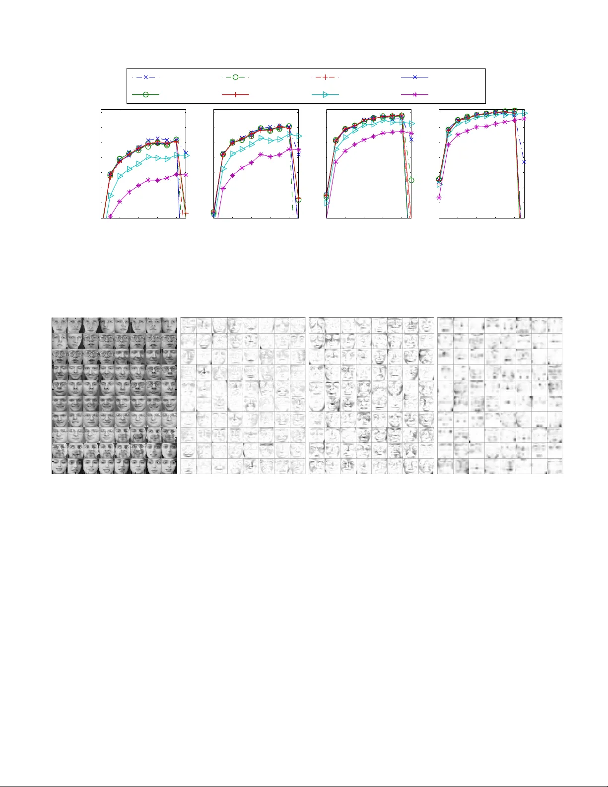
Original Paper
Loading high-quality paper...
Comments & Academic Discussion
Loading comments...
Leave a Comment