On the complexity of piecewise affine system identification

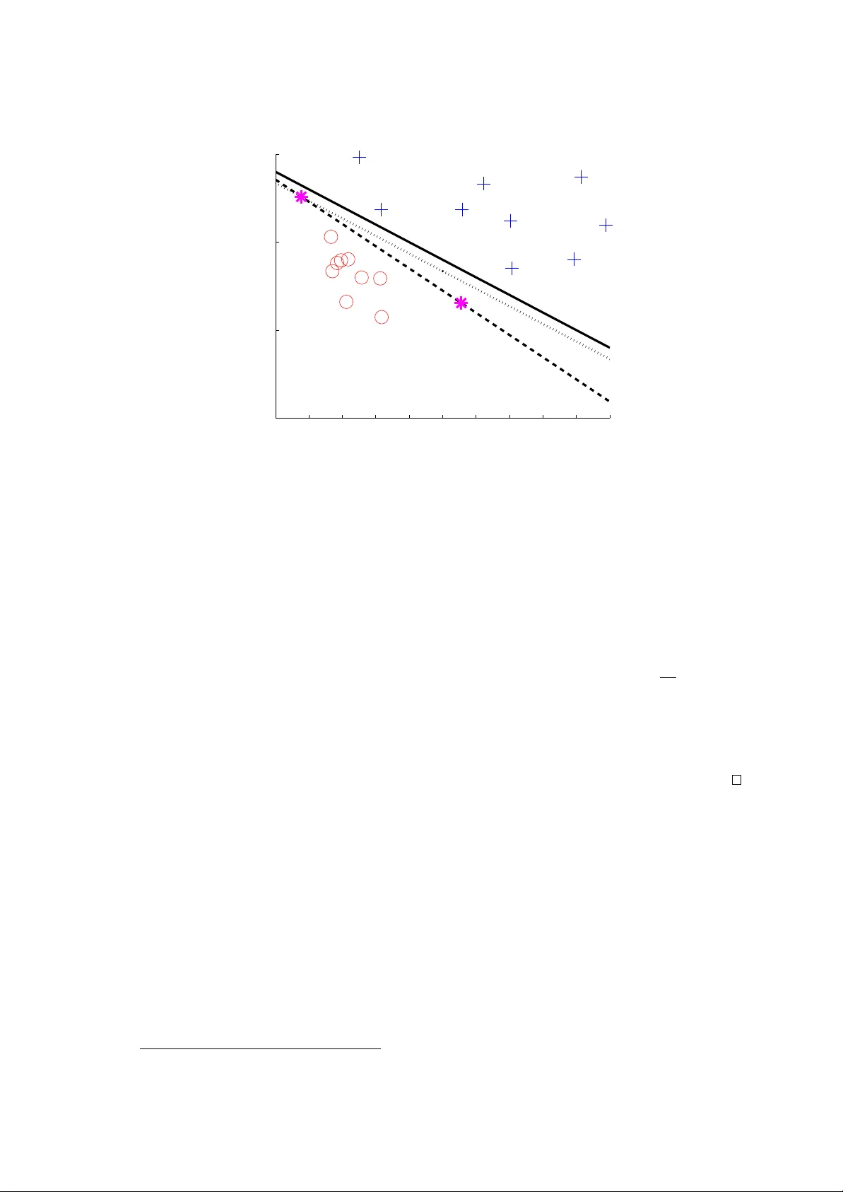
On the complexit y of piecewise affine system iden tification F abien Lauer Univ ersit ´ e de Lorraine, CNRS, LORIA, UMR 7503, F-54506 V andœuvre-l` es-Nancy , F rance July 23, 2018 Abstract The pap er provides results regarding the computational complexity of hybrid system iden- tification. More precisely , w e focus on the estimation of piecewise affine (PW A) maps from input-output data and analyze the complexit y of computing a global minimizer of the error. Previous w ork show ed that a global solution could be obtained for contin uous PW A maps with a worst-case complexity exponential in the n umber of data. In this pap er, we show how global optimalit y can b e reac hed for a slightly more general class of possibly discontin uous PW A maps with a complexity only p olynomial in the num b er of data, how ever with an exp onen tial complexit y with resp ect to the data dimension. This result is obtained via an analysis of the in trinsic classification subproblem of asso ciating the data p oin ts to the differen t mo des. In addition, we prov e that the problem is NP-hard, and thus that the exp onen tial complexity in the dimension is a natural exp ectation for any exact algorithm. 1 In tro duction Hybrid system identification aims at estimating a mo del of a system switching b et ween different op erating mo des from input-output data. More precisely , most of the literature considers autore- gressiv e with external input (ARX) mo dels to cast the problem as a regression one [1]. Then, t w o cases can be distinguished: switc hing regression, where the system arbitrarily switc hes from one mo de to another, and piecewise affine (PW A) regression, where the switc hes dep end on the regressors. A n um b er of metho ds with satisfactory performance in practice are now a v ailable for these problems [2]. Ho wev er, compared with linear system iden tification, a ma jor w eakness of these metho ds is their lack of guaran tees. F or the particular case of noiseless data, the algebraic metho d [3] pro vides a solution to switching regression with a small n umber of mo des. How ever, the qualit y of the estimates quic kly degrades with the increase of the noise level. A few sparsity-based methods [4, 5] also offer guarantees in the noiseless case, but these are sub ject to a condition on b oth the data and the sought solution. In the presence of noise, most methods consider the minimization of the error of the mo del ov er the data [1]. While this do es not necessarily yields the b est predictive mo del (due to issues like iden tifiability , p ersistence of excitation and access to a limited amoun t of data), obtaining statistical guaran tees with such an approach has a long history in statistics and system identification [6]. How ever, such results are not av ailable for hybrid systems. This is probably due to the fact that minimizing the error of a h ybrid model is a difficult noncon vex optimization problem inv olving the simultaneous classification of the data p oin ts into mo des and the regression of a submo del for each mo de. Thus, theoretical guaran tees could only b e obtained under the rather strong assumption that this problem has been solv ed to global optimalit y and most of the literature [7, 8, 9, 10, 11, 12] fo cuses on this issue with heuristics of v arious degrees of accuracy and computational efficiency . Many recent w orks [4, 13, 14, 15, 16, 5] try to av oid lo cal minima b y considering conv ex formulations, but these only yield optimalit y with respect to a relaxation of the original problem. Global optimality in the presence of noise was only reac hed in [17] for a particular class of con tinuous PW A maps kno wn as hinging-hyperplanes by reformulating the problem as a mixed-in teger program solved by 1 branc h-and-b ound tec hniques. How ever, suc h optimization problems are NP-hard [18] and branch- and-b ound algorithms ha v e a w orst-case complexity exponential in the n um b er of in teger v ariables, here prop ortional to the n umber of data and the num b er of modes. Inspired b y related clustering problems, suc h as the minimization of the sum of squared distances b et ween p oin ts and their group centers, we could minimize the hybrid mo del error by en umerating all p ossible classifications of the p oin ts. But the n umber of classifications is exp onen tial in the n um b er of data. Con v ersely , the other approach enumerating a sample of v alues for the real v ariables of the problem is exp onen tial in the dimension and can only offer an appro ximate solution. Ov erall, the literature do es not pro vide a metho d that can guaran tee both the optimality and the computabilit y of a global minimizer of the error, while the computational complexity of this problem remains unknown and cannot b e deduced from the NP-hardness of classical clustering problems [19] (see [18, 20] for an introduction to computational complexit y and its relev ance to con trol theory). Con tribution The pap er pro vides t wo results regarding the computational complexity of PW A regression, and more precisely for the problem of finding a global minimizer of the error of a PW A mo del, formalized in Sect. 2. First, w e sho w in Sect. 3 that the problem is NP-hard. Then, w e show in Sect. 4 that, for an y fixed dimension of the data, an exact solution can b e computed in time p olynomial in the n umber of data via an en umeration of all possible classifications. T o obtain this result and av oid the exp onen tial gro wth of the n um b er of classifications with the n umber of data, w e sho w that, in PW A regression, the classification of the data points is highly constrained and the num b er of classifications to test can b e limited. The price to pa y for this gain is an exp onen tial complexit y with resp ect to the data dimension and the n umber of mo des. F uture work is outlined in Sect. 5. Notations W e use the indicator function 1 E of an even t E that is 1 if the even t o ccurs and 0 otherwise. W e define sign( u ) = 1 if u ≥ 0 and − 1 otherwise. Given a set of lab els Q ⊂ Z and a set of N p oin ts, a lab eling of these p oints is any q ∈ Q N . W e use j = argmax k ∈Q u ( k ) as a shorthand for j = min { l ∈ argmax k ∈Q u ( k ) } . Given tw o sets, X and Y , Y X is the set of functions from X to Y . 2 Problem formulation As in most w orks, we concen trate on discrete-time PW ARX system iden tification considered as a PW A regression problem with regression vectors x i = [ y i − 1 , . . . , y i − n y , u i , . . . , u i − n u ] T ∈ X built from past inputs u i − k and outputs y i − k . Since we are interested in computational complexity results, w e restrain the data to rational, digitally representable, v alues and set X ⊆ Q d . The outputs are assumed to b e generated b y a PW A system f as y i = f ( x i ) + v i , where v i is a noise term. More precisely , PW A mo dels can b e expressed via a set of n affine submo dels and a function h : X → Q = { 1 , . . . , n } determining the activ e submo del: f ( x ) = w T h ( x ) x , where x = [ x T , 1] T . W e call the function h a classifier as it classifies the data p oin ts in the differen t mo des. Typically , PW A systems are defined with h implementing a p olyhedral partition of X , with mo des possibly spanning unions of polyhedra. Ho wev er, in most of the literature on PW A system identification [1, 7, 8, 9, 16], h is estimated within the family of linear classifiers H = { h ∈ Q X : h ( x ) = argmax k ∈Q h T k x + b k , h k ∈ Q d , b k ∈ Q } , (1) based on a set of n linear functions and for whic h a mo de spanning a union of polyhedra must b e mo deled as sev eral mo des with similar affine submo dels. F or PW A maps with n = 2 modes, h is a binary classifier for which it is common to consider its output in Q = {− 1 , +1 } instead of { 1 , 2 } . Such a binary classifier can b e obtained b y taking the sign of a real-v alued function. If this function is linear (or affine), then w e obtain a linear classifier, whic h is equiv alent to a separating h yp erplane dividing the input space X in t wo half-spaces. In this case, the function class H can b e defined as H = { h ∈ Q X : h ( x ) = sign( h T x + b ) , h ∈ Q d , b ∈ Q } (2) 2 with a single set of parameters ( h , b ) corresp onding to the normal to the hyperplane and the offset from the origin. An equiv alence with the m ulti-class form ulation in (1) is obtained b y using h = h 1 − h 2 and b = b 1 − b 2 . In this pap er, we consider the common estimation approach of minimizing the error on N data pairs ( x i , y i ) ∈ X × Q , measured p oin twise by a loss function ` : Q → Q + as ` ( y i − f ( x i )) = X j ∈Q 1 h ( x i )= j ` ( y i − w T j x i ) . More precisely , we foc us on well-posed instances of the problem where N is significan tly larger than the dimension d and the num b er of mo des n is giv en. Indeed, with free n the problem is ill-p osed as the solution is only defined up to a trade-off b et ween the num b er of mo des and the mo del accuracy . F or the conv erse well-posed approach that minimizes n for a given error bound, a complexity analysis can be found in [21]. Under these assumptions, the problem is as follows. Problem 1 (Error-minimizing PW A regression) . Given a data set { ( x i , y i ) } N i =1 ∈ ( X × Q ) N with X ⊆ Q d and an inte ger n ∈ [2 , N / ( d + 1)] , find a glob al solution to min w ∈ Q n ( d +1) ,h ∈H 1 N N X i =1 X j ∈Q 1 h ( x i )= j ` ( y i − w T j x i ) , (3) wher e w = ( w j ) j ∈Q is the c onc atenation of al l p ar ameter ve ctors and H ⊂ Q X is the set of n -c ate gory line ar classifiers as in (1) or (2) . The follo wing analyzes the time complexit y of Problem 1 under the classical mo del of com- putation kno wn as a T uring machine [18]. The time complexit y of a problem is the low est time complexit y of an algorithm solving any instance of that problem, where the time complexity of an algorithm is the maximal num b er of steps o ccuring in the computation of the corresp onding T uring machine program. The loss function ` is assumed to b e computable in p olynomial time throughout the pap er. 3 NP-hardness This section con tains the pro of of the following NP-hardness result, where an NP-hard problem is one that is at least as hard as any problem from the class NP of nondeterministic p olynomial time decision problems [18] (NP is the class of all decision problems for whic h a solution can b e certified in p olynomial time). Theorem 1. With a loss function ` such that ` ( e ) = 0 ⇔ e = 0 , Pr oblem 1 is NP-har d. The pro of uses a reduction from the partition problem, kno wn to b e NP-complete [18], i.e., a problem that is both NP-hard and in NP . Problem 2 (P artition) . Given a multiset (a set with p ossibly multiple instanc es of its elements) of d p ositive inte gers, S = { s 1 , . . . , s d } , de cide whether ther e is a multisubset S 1 ⊂ S such that X s i ∈ S 1 s i = X s i ∈ S \ S 1 s i . More precisely , we will reduce Problem 2 to the decision form of Problem 1. Problem 3 (Decision form of PW A regression) . Given a data set { ( x i , y i ) } N i =1 ∈ ( X × Q ) N , an inte ger n ∈ [2 , N / ( d + 1)] and a thr eshold  ≥ 0 , de cide whether ther e is a p air ( w , h ) ∈ Q n ( d +1) × H such that 1 N N X i =1 X j ∈Q 1 h ( x i )= j ` ( y i − w T j x i ) ≤ , (4) wher e H is the set of line ar classifiers as in (1) or (2) and the loss function ` is such that ` ( e ) = 0 ⇔ e = 0 . 3 Prop osition 1. Pr oblem 3 is NP-c omplete. Pr o of. Since given a candidate pair ( w , h ) the condition (4) can b e verified in p olynomial time, Problem 3 is in NP . Then, the pro of of its NP-completeness pro ceeds b y showing that the P artition Problem 2 has an affirmative answer if and only if Problem 3 with  = 0 has an affirmative answ er. Giv en an instance of Problem 2, let N = 2 d + 3, n = 2, Q = {− 1 , 1 } and build a data set with ( x i , y i ) =                ( s i e i , s i ) , if 1 ≤ i ≤ d ( − s i − d e i − d , s i − d ) , if d < i ≤ 2 d ( s , 0) , if i = 2 d + 1 ( − s , 0) , if i = 2 d + 2 ( 0 , 0) , if i = 2 d + 3 , where e k is the k th unit vector of the canonical basis for Q d and s = P d k =1 s k e k . If Problem 2 has an affirmative answer, then, using the notations of (2), w e can set w 1 = X k ∈ I 1 e k − X k ∈ I − 1 e k , w − 1 = − w 1 , h = X k ∈ I 1 e k − X k ∈ I − 1 e k , b = 0 , where e k = [ e T k , 0] T , I 1 is the set of indexes of the elements of S in S 1 and I − 1 = { 1 , . . . , d } \ I 1 . This gives w T 1 x i =                          s i = y i , if i ≤ d and i ∈ I 1 − s i , if i ≤ d and i ∈ I − 1 s i − d = y i , if i > d and i − d ∈ I − 1 − s i − d , if i > d and i − d ∈ I 1 P k ∈ I 1 s k − P k ∈ I − 1 s k = 0 = y i , if i = 2 d + 1 P k ∈ I − 1 s k − P k ∈ I 1 s k = 0 = y i , if i = 2 d + 2 0 = y i , if i = 2 d + 3 and we can similarly sho w that w T − 1 x i = y i , if i ∈ I − 1 ∨ i − d ∈ I 1 ∨ i > 2 d, while h T x i is p ositiv e if i ∈ I 1 ∨ i − d ∈ I − 1 and negative if i ∈ I − 1 ∨ i − d ∈ I 1 . Therefore, for all p oin ts, w T h ( x i ) x i = y i , i = 1 , . . . , 2 d + 3, and the cost function of Problem 1 is zero, yielding an affirmativ e answer for Problem 3. It remains to pro v e that if (4) holds with  = 0, then Problem 2 has an affirmativ e answ er. T o see this, note that due to ` b eing p ositiv e, a zero cost implies a zero loss for all data p oin ts. Thus, b y ` ( e ) = 0 ⇔ e = 0, if (4) holds with  = 0, w T h ( x i ) x i = y i , i = 1 , . . . , 2 d + 3 . (5) Also note that if h ( x i ) = h ( x i + d ) = 1 for some i ≤ d , we ha ve s i w 1 ,i + w 1 ,d +1 = − s i w 1 ,i + w 1 ,d +1 = s i . This is only p ossible if s i = 0, which is not the case (otherwise w e can simply remov e s i without influencing the partition problem), or if w 1 ,d +1 = s i . The latter is imp ossible if h ( x i ) = h ( x i + d ) since h is a linear classifier that m ust return the same category for all p oin ts on the line segment b et ween x i and x i + d , which includes the origin x 2 d +3 = 0 and thus would imply by (5) that w T 1 x 2 d +3 = w 1 ,d +1 = y 2 d +3 = 0. As a consequence, h ( x i ) = h ( x i + d ) = 1 cannot hold, and since w e can similarly show that h ( x i ) = h ( x i + d ) = − 1 cannot hold, we hav e h ( x i ) 6 = h ( x i + d ) for all i ≤ d . Hence, (5) leads to w T 1 x i 6 = y i ⇒ w T 1 x d + i = y d + i , i = 1 , . . . , d (6) w T − 1 x i 6 = y i ⇒ w T − 1 x d + i = y d + i , i = 1 , . . . , d. (7) 4 Let ˆ I 1 = { i ∈ { 1 , . . . , d } : w T 1 x i = y i } and ˆ I − 1 = { 1 , . . . , d } \ ˆ I 1 . Then, if h ( x 2 d +3 ) = +1, w 1 ,d +1 = 0 and for all i ≤ d , w T 1 x i = w i s i . Therefore, for all i ∈ ˆ I 1 , w i = 1, while for all i ∈ ˆ I − 1 , (6) gives w T 1 x d + i = y d + i , i.e., − w i s i = s i and w i = − 1. This leads to w T 1 x 2 d +1 = X i ∈ ˆ I 1 s i − X i ∈ ˆ I − 1 s i = − w T 1 x 2 d +2 . Th us, if w T 1 x 2 d +1 = y 2 d +1 = 0 or w T 1 x 2 d +2 = y 2 d +2 = 0, a v alid partition in the sense of Problem 2 is obtained with S 1 = { s i } i ∈ ˆ I 1 . In addition, if w T 1 x 2 d +1 6 = 0 and w T 1 x 2 d +2 6 = 0, then b y (5), w T − 1 x 2 d +1 = w T − 1 x 2 d +2 = 0, which by construction implies that w − 1 ,d +1 = 0. In this case, we redefine ˆ I − 1 = { i ∈ { 1 , . . . , d } : w T − 1 x i = y i } and ˆ I 1 = { 1 , . . . , d } \ ˆ I − 1 to obtain w − 1 ,i = 1 for all i ∈ ˆ I − 1 and w − 1 ,i = − 1 for all i ∈ ˆ I 1 , resulting also in a v alid partition by the fact that w T − 1 x 2 d +2 = P i ∈ ˆ I 1 s i − P i ∈ ˆ I − 1 s i = 0. Since a similar reasoning applies to the case h ( x 2 d +3 ) = − 1 b y symmetry (substituting w − 1 for w 1 ), a zero cost, i.e., (4) with  = 0, alw ays implies an affirmative answ er to Problem 2. Pr o of of The or em 1. Since the decision form of Problem 1 with ` ( e ) = 0 ⇔ e = 0, i.e., Problem 3, is NP-complete, Problem 1 with such a loss function is NP-hard (solving Problem 1 also yields the answ er to Problem 3 and th us it is at least as hard as Problem 3). 4 P olynomial complexit y in the num b er of data W e no w state the result regarding the p olynomial complexit y of Problem 1 with respect to N under the follo wing assumptions, the first of which holds almost surely for randomly dra wn data p oin ts, while the second one holds for instance for ` ( e ) = e 2 with a linear time complexity T ( N ) = Ø( N ) [22]. Assumption 1. The p oints { x i } N i =1 ar e in gener al p osition, i.e., no hyp erplane of Q d c ontains mor e than d p oints. Assumption 2. Given { ( x i , y i ) } N i =1 ∈ ( X × Q ) N , the pr oblem min v ∈ Q d +1 P N i =1 ` ( y i − v T x i ) has a p olynomial time c omplexity T ( N ) for any fixe d inte ger d ≥ 1 . Theorem 2. F or any fixe d numb er of mo des n and dimension d , under Assumptions 1 – 2, the time c omplexity of Pr oblem 1 is no mor e than p olynomial in the numb er of data N and in the or der of T ( N )Ø  N dn ( n − 1) / 2  . The pro of of Theorem 2 relies on the existence of exact algorithms with complexity p olynomial in N for the binary case ( n = 2, Prop osition 4) and the multi-class case ( n ≥ 3, Corollary 1). These algorithms are based on a reduction of Problem 1 to a com binatorial search in tw o steps. The first step reduces the problem to a classification one. Indeed, Problem 1 can be reform ulated as the searc h for the classifier h , since b y fixing h , the optimal parameter vectors { w j } j ∈Q can b e obtained by solving n indep enden t linear regression problems on the subsets of data resulting from the classification by h , which, b y Assumption 2, can b e p erformed in the p olynomial time T ( N ). This yields the follo wing reform ulation of the problem. Prop osition 2. Pr oblem 1 is e quivalent to min w ∈ Q n ( d +1) ,h ∈H 1 N N X i =1 X j ∈Q 1 h ( x i )= j `  y i − w T j x i  (8) s.t. ∀ j ∈ Q , w j ∈ argmin v ∈ Q d +1 N X i =1 1 h ( x i )= j ` ( y i − v T x i ) . The second step reduces the estim ation of h to a combinatorial problem solv ed in Ø  N dn ( n − 1) / 2  op erations, as detailed in Sect. 4.1 – 4.2 for n = 2 and in Sect. 4.3 for n ≥ 3. 5 4.1 Finding the optimal classification W e reduce the complexit y of searching for the classifier b y considering all possible linear classifi- cations instead of all p ossible linear classifiers. In other words, we pro ject the class H of classifiers on to the set of p oin ts S = { x i } N i =1 to reduce a contin uous search to a combinatorial problem. This is in line with the tec hniques used in statistical learning theory [23] for the differen t purp ose of computing error b ounds for infinite function classes. Thus, we in tro duce definitions from this field. Definition 1 (Pro jection onto a set) . The pr oje ction of a set of classifiers H ⊂ Q X onto S = { x i } N i =1 , denote d H S , is the set of al l lab elings of S that c an b e pr o duc e d by a classifier in H : H S = { ( h ( x 1 ) , . . . , h ( x N )) : h ∈ H} ⊆ Q N . Definition 2 (Gro wth function) . The growth function Π H ( N ) of H at N is the maximal numb er of lab elings of N p oints that c an b e pr o duc e d by classifiers fr om H : Π H ( N ) = sup S ∈X N |H S | . W e no w focus on binary PW A maps and th us on binary classifiers with output in Q = {− 1 , +1 } . F or suc h classifiers, we ob viously ha ve Π H ( N ) ≤ 2 N for all N . By further restricting H to affine classifiers as in (2), results from statistical learning theory (see, e.g., [23]) provide the tigh ter b ound Π H ( N ) ≤  eN d +1  d +1 , whic h is p olynomial in N and thus promising from the viewpoint of global optimization. How ever, its pro of is not constructiv e and do es not pro vide an explicit algorithm for en umerating all the lab elings. The following theorem, though leading to a lo oser bound on the gro wth function, offers a constructive scheme to compute the pro jection H S , which is what we need in order to test all the labelings in H S for global optimization. Theorem 3. The gr owth function of the class of binary affine classifiers of Q d , H in (2) , is b ounde d for any N > d by Π H ( N ) ≤ 2 d +1  N d  = Ø( N d ) and, for any set S of N p oints in gener al p osition, an algorithm builds the pr oje ction H S in Ø( N d ) time. The pro of of Theorem 3 relies on the follo wing prop osition, whic h is illustrated b y Fig. 1. Prop osition 3. F or any binary affine classifier h in H (2) and any finite set of N > d p oints S = { x i } N i =1 in gener al p osition, ther e is a subset of p oints S h ⊂ S of c ar dinality | S h | = d and a sep ar ating hyp erplane of p ar ameters ( h S h , b S h ) p assing thr ough the p oints in S h , i.e., ∀ x ∈ S h , h T S h x + b S h = 0 , with k h S h k = 1 , (9) which yields the same classific ation of S in the sense that ∀ x i ∈ S \ S h , h ( x i ) = sign ( h T S h x i + b S h ) . (10) Pr o of sketch. F or all classifiers h with separating hyperplanes passing through d p oin ts of S , the statement is ob vious. F or the others passing through p p oin ts with 0 ≤ p < d , they can be transformed to pass through additional p oin ts without changing the classification of the remaining p oin ts. If p = 0, it suffices to translate the hyperplane to the closest p oin t. If 0 < p < d , the h yp erplane can be rotated with a plane of rotation that leav es unchanged the subspace spanned by the p p oin ts and a minimal angle yielding a rotated h yp erplane passing through p 0 > p p oin ts, where p 0 ≤ d b y the general p osition assumption. Iterating this sc heme until p = d yields a hyperplane passing through the points in S h of parameters ( h S h , b S h ) satisfying (9) and (10). W e can now prov e Theorem 3. 6 −5 −4 −3 −2 −1 0 1 2 3 4 5 −10 −5 0 5 Figure 1: The h yp erplane H (plain line) pro duces the same classification (in to + and ◦ ) as the h yp erplane H S (dashed line) obtained by a translation (dotted line) and a rotation of H such that it passes through exactly 2 points of S ( ∗ ). Pr o of of The or em 3. F or any lab eling q in H S , there is a classifier h ∈ H that pro duces this lab eling. Applying Prop osition 3 to h , w e obtain another classifier h S h of parameters ( h S h , b S h ) that passes through the p oin ts in S h and that agrees with h on S \ S h . Let ˆ q ∈ {− 1 , +1 } N b e defined b y ˆ q i = h S h ( x i ), i = 1 , . . . , N . Then, w e generate 2 d lab elings by setting its entries ˆ q i with i ∈ S h to all the 2 d com binations of signs (recall that | S h | = d ). By construction, there is no lab eling of S that agrees with q on S \ S h other than these 2 d lab elings. Since this holds for any q ∈ H S , the cardinality of H S cannot be larger than 2 d times the num b er of hyperplanes passing through d points of S . Since eac h subset S h ⊂ S of cardinalit y d giv es rise to t wo h yp erplanes of opp osite orien tations, the n umber of such hyperplanes is 2  N d  and w e ha ve Π H ( N ) ≤ 2 d +1  N d  < 2 d +1 N d d ! = Ø( N d ). In addition, there is an algorithm that enumerates all the subsets S h in  N d  iterations and builds H S b y computing a hyperplane passing through the p oin ts 1 in S h and the corresp onding 2 d +1 lab elings at eac h iteration. Since these inner computations can b e p erformed in constan t time with resp ect to N , the algorithm has a time complexity in the order of  N d  = Ø( N d ). 4.2 Global optimization of binary PW A mo dels W e can use the results ab o ve to reduce the complexit y of Problem 1 in the binary case, considered in the following in its equiv alent form (8) from Prop osition 2. First, note that the cost function in (8) only dep ends on h , since all feasible v alues of w for a giv en h yield the same cost. F urthermore, the cost do es not dep end on the exact v alue of h , but only on the resulting classification, i.e., on h ( x i ), i = 1 , . . . , N . Thus, given a global solution h ∗ to (8), any classifier h pro ducing the same classification yields the same cost function v alue and hence is also a global solution. Thus, the problem reduces to the search for the correct classification q ∈ H S , whose complexit y is in Ø(Π H ( N )) and b ounded by Theorem 3. In addition, for the purp ose of binary PW A regression, opp osite lab elings q and − q are equiv alent and can b e pruned from H S . This is due to the symmetry of the cost function (8). Algorithm 1 pro vides a solution to Problem 1 for the binary case while taking this symmetry in to accoun t. 1 The normal h of a h yp erplane { x : h T x + b = 0 } passing through d p oin ts { x i } d i =1 in Q d can b e computed as a unit v ector in the n ull space of [ x 2 − x 1 , . . . , x d − x 1 ] T , while the offset is given b y b = − h T x i for an y of the x i ’s. 7 Algorithm 1 Exact solution to Problem 1 for n = 2 Input: A data set { ( x i , y i ) } N i =1 ⊂ ( Q d × Q ) N . Initialize S ← { x i } N i =1 and J ∗ ← + ∞ . for all S h ⊂ S suc h that | S h | = d do Compute the parameters ( h S h , b S h ) of a h yp erplane passing through the p oin ts in S h . Classify the data points: S 1 = { x i ∈ S : h T S h x i + b S h > 0 } , S 2 = { x i ∈ S : h T S h x i + b S h < 0 } . for all classification of S h in to S 1 h and S 2 h do Set w j ∈ argmin v ∈ Q d +1 X x i ∈ S j ∪ S j h ` ( y i − v T x i ) , j = 1 , 2 , J = 1 N 2 X j =1 X x i ∈ S j ∪ S j h ` ( y i − w T j x i ) , and up date the b est solution ( J ∗ ← J, w ∗ ← [ w T 1 , w T 2 ] T , h ∗ ← h S h , b ∗ ← b S h ) if J < J ∗ . end for end for return w ∗ , h ∗ , b ∗ . Prop osition 4. Under Assumptions 1 – 2, Algorithm 1 exactly solves Pr oblem 1 for n = 2 and any fixe d d with a p olynomial c omplexity in the or der of T ( N )Ø( N d ) . Pr o of. By following a similar path as for Theorem 3, Algorithm 1 can b e pro ved to test all linear classifications of the data p oints up to symmetric ones. Since Algorithm 1 computes a solution in terms of w that is feasible for (8) for eac h of these classifications, the v alue of J coincides with the cost function of (8) for a particular h . By the symmetry of this cost function with respect to h and the fact that it only depends on h via its v alues at the data p oin ts, Algorithm 1 computes all p ossible v alues of the cost function, including the exact global optim um of (8), and returns a global minimizer. Thus, by Prop osition 2, it also solves Problem 1. The total n um b er of iterations of Algorithm 1 is 2 d  N d  = Ø( N d ) and, under Assumption 2, these iterations only in volv e operations computed in p olynomial time in the order of T ( N ), hence the ov erall time complexity in the order of T ( N )Ø( N d ). 4.3 Multi-class extension F or n > 2, the b oundary b et ween 2 modes j and k > j implemen ted by a linear classifier from H in (1) is a hyperplane of equation h j k ( x ) = h j ( x ) − h k ( x ) = 0, i.e., based on the difference of the tw o functions h j ( x ) = h T j x + b j and h k ( x ) = h T k x + b k . Based on these h yp erplanes, the classification rule can b e written as h ( x ) = argmax k ∈Q h k ( x ) = j, such that ( h j k ( x ) ≥ 0 , ∀ k > j, h kj ( x ) < 0 , ∀ k < j. Based on these facts, we can build an algorithm to recov er all p ossible classifications consistent with a linear classification in the sense of (1). Theorem 4. F or the set of multi-class line ar classifiers of Q d , H in (1) , the gr owth function is b ounde d for any N > d by Π H ( N ) ≤  2 d +1  N d  n ( n − 1) / 2 = Ø( N dn ( n − 1) / 2 ) and, for any set S of N p oints of Q d in gener al p osition, an algorithm builds H S in Ø( N dn ( n − 1) / 2 ) time. 8 Pr o of. Any classification produced b y a classifier from (1) can b e computed from the signs of the n H = n ( n − 1) / 2 functions h j k = h j − h k , 1 ≤ j < k ≤ n , corresp onding to the pairwise separating h yp erplanes. F or an y S , for each of these hyperplanes, Prop osition 3 provides an equiv alent binary classifier which must b e one from the 2  N d  h yp erplanes passing through d points S j k of S . The n um b er of sets of n H suc h h yp erplanes is 2 n H  N d  n H . Since these classifiers cannot pro duce all the 2 n H d classifications of the n H d p oin ts in the sets S j k , we must also take these into account so that the num b er of classifications of S is upp er b ounded b y |H S | ≤ 2 n H d 2 n H  N d  n H = Ø( N dn H ). This upp er b ound holds for any S , and thus also applies to the growth function. Finally , an algorithm that makes explicit all the classifications mentioned abov e to build H S can b e constructed in a recursiv e manner, with one classification per iteration and thus with a similar n umber of iterations, eac h one including computations p erformed in constan t time. Theorem 4 implies the following for PW A regression. Corollary 1. Under Assumptions 1 – 2, a glob al solution to Pr oblem 1 with n ≥ 3 c an b e c ompute d with a p olynomial c omplexity in the or der of T ( N )Ø( N dn ( n − 1) / 2 ) . 5 Conclusions The pap er discussed complexit y issues for PW A regression and show ed that i) the global minimiza- tion of the error is NP-hard in general, and ii) for fixed num b er of mo des and data dimension, an exact solution can b e obtained in time polynomial in the n umber of data. The pro of of NP-hard ness also implies that the problem remains NP-hard ev en when the n umber of mo des is fixed to 2, which indicates that the complexit y is mostly due to the data dimension. An op en issue concerns the conditions under whic h a PW A system generates tra jectories satisfying the general p osition as- sumption used by the p olynomial-time algorithm. F uture work will also focus on the extension of the results to the case of arbitrarily switc hed systems and heuristics inspired b y the p olynomial- time algorithm, whose practical application remains limited b y an exp onen tial complexit y in the dimension. Ac kno wledgemen ts The author would like to thank the anon ymous reviewers for their comments and suggestions. Thanks are also due to Y ann Guermeur for carefully reading this manuscript. References [1] S. Paoletti, A. L. Juloski, G. F errari-T recate, R. Vidal, Identification of hybrid systems: a tutorial, Europ ean Journal of Con trol 13 (2-3) (2007) 242–262. [2] A. Garulli, S. Paoletti, A. Vicino, A survey on switched and piecewise affine system iden- tification, in: Pro c. of the 16th IF A C Symp. on System Identification (SYSID), 2012, pp. 344–355. [3] R. Vidal, S. Soatto, Y. Ma, S. Sastry , An algebraic geometric approach to the identification of a class of linear hybrid systems, in: Pro c. of the 42nd IEEE Conf. on De cision and Control (CDC), Maui, Haw a ¨ ı, USA, 2003, pp. 167–172. [4] L. Bak o, Iden tification of switc hed linear systems via sparse optimization, Automatica 47 (4) (2011) 668–677. [5] I. Maruta, H. Ohlsson, Compression based identification of PW A systems, in: Pro c. of the 19th IF AC W orld Congress, Cape T own, South Africa, 2014, pp. 4985–4992. 9 [6] L. Ljung, System identification: Theory for the User, 2nd Edition, Prentice Hall, 1999. [7] G. F errari-T recate, M. Muselli, D. Lib erati, M. Morari, A clustering technique for the identi- fication of piecewise affine systems, Automatica 39 (2) (2003) 205–217. [8] A. Bemp orad, A. Garulli, S. Paoletti, A. Vicino, A b ounded-error approac h to piecewise affine system iden tification, IEEE T ransactions on Automatic Control 50 (10) (2005) 1567–1580. [9] A. L. Juloski, S. W eiland, W. Heemels, A Ba y esian approach to identification of hybrid sys- tems, IEEE T ransactions on Automatic Control 50 (10) (2005) 1520–1533. [10] F. Lauer, G. Bloch, R. Vidal, A contin uous optimization framework for hybrid system iden ti- fication, Automatica 47 (3) (2011) 608–613. [11] F. Lauer, Estimating the probabilit y of success of a simple algorithm for switched linear regres- sion, Nonlinear Analysis: Hybrid Systems 8 (2013) 31–47, supplemen tary material av ailable at http://www.loria.fr/ ~ lauer/klinreg/ . [12] T. Pham Dinh, H. Le Thi, H. Le, F. Lauer, A difference of conv ex functions algorithm for switc hed linear regression, IEEE T ransactions on Automatic Control 59 (8) (2014) 2277–2282. [13] N. Oza y , M. Sznaier, C. Lagoa, O. Camps, A sparsification approach to set mem b ership iden tification of switched affine syste ms, IEEE T ransactions on Automatic Con trol 57 (3) (2012) 634–648. [14] H. Ohlsson, L. Ljung, S. Boyd, Segmentation of ARX-models using sum-of-norms regulariza- tion, Automatica 46 (6) (2010) 1107–1111. [15] H. Ohlsson, L. Ljung, Identification of switc hed linear regression mo dels using sum-of-norms regularization, Automatica 49 (4) (2013) 1045–1050. [16] F. Lauer, V. L. Le, G. Blo c h, Learning smo oth mo dels of nonsmo oth functions via conv ex optimization, in: Pro c. of the IEEE Int. W orkshop on Mac hine Learning for Signal Pro cessing (MLSP), Santander, Spain, 2012. [17] J. Roll, A. Bemporad, L. Ljung, Identification of piecewise affine systems via mixed-integer programming, Automatica 40 (1) (2004) 37–50. [18] M. Garey , D. Johnson, Computers and Intractabilit y: a Guide to the Theory of NP- Completeness, W.H. F reeman and Compan y , 1979. [19] D. Aloise, A. Deshpande, P . Hansen, P . Popat, NP-hardness of Euclidean sum-of-squares clustering, Machine Learning 75 (2) (2009) 245–248. [20] V. Blondel, J. Tsitsiklis, A survey of computational complexity results in systems and con trol, Automatica 36 (9) (2000) 1249–1274. [21] R. Alur, N. Singhania, Precise piecewise affine mo dels from input-output data, in: Proc. of the 14th Int. Conf. on Embedded Soft ware (EMSOFT), 2014. [22] G. H. Golub, C. F. V an Loan, Matrix Computations, 4th Edition, John Hopkins Universit y Press, 2013. [23] V. V apnik, Statistical Learning Theory , John Wiley & Sons, 1998. 10