Quantization based Fast Inner Product Search

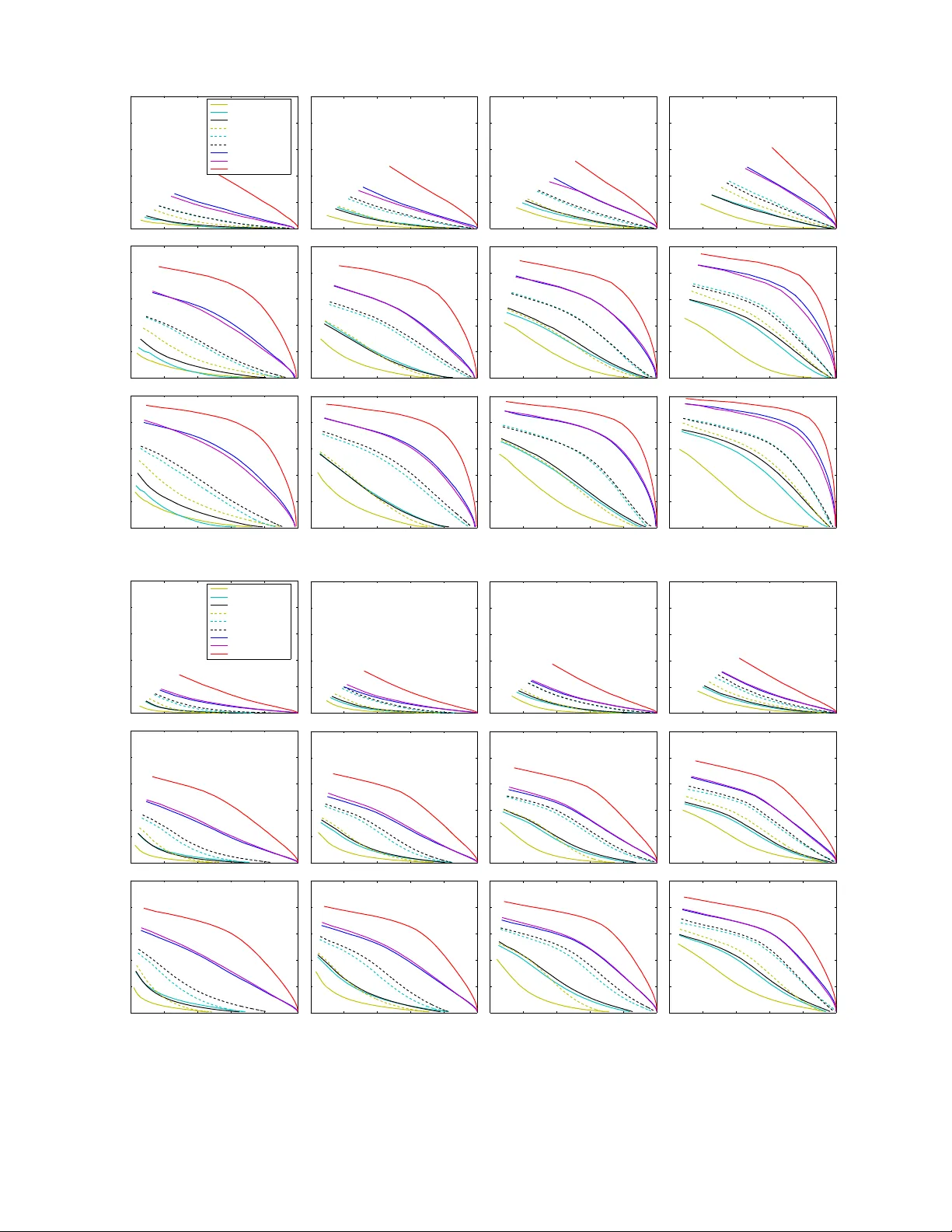
Quantization based F ast Inner Product Search Ruiqi Guo, Sanji v Kumar , Krzysztof Choromanski, David Simcha Google Research, Ne w Y ork, NY 10011, USA { guorq, sanjivk, kchoro, dsimcha } @google.com Abstract W e propose a quantization based approach for fast approximate Maximum Inner Product Search (MIPS). Each database v ector is quantized in multiple subspaces via a set of codebooks, learned directly by minimizing the inner product quantization error . Then, the inner product of a query to a database vector is approximated as the sum of inner products with the subspace quantizers. Dif ferent from recently proposed LSH approaches to MIPS, the database vectors and queries do not need to be augmented in a higher dimensional feature space. W e also provide a theoretical analysis of the proposed approach, consisting of the concentration results under mild assumptions. Furthermore, if a small sample of example queries is giv en at the training time, we propose a modified codebook learning procedure which further improves the accuracy . Experimental results on a variety of datasets including those arising from deep neural networks sho w that the proposed approach significantly outperforms the existing state-of-the-art. 1 Intr oduction Many information processing tasks such as retrie v al and classification in volve computing the inner product of a query vector with a set of database vectors, with the goal of returning the database instances having the largest inner products. This is often called Maximum Inner Product Search (MIPS) problem. Formally , given a database X = { x i } i =1 ··· n , and a query vector q drawn from the query distribution Q , where x i , q ∈ R d , we want to find x ∗ q ∈ X such that x ∗ q = argmax x ∈ X ( q T x ) . This definition can be trivially e xtended to return top- N largest inner products. The MIPS problem is particularly appealing for large scale applications. For example, a recommendation system needs to retrie ve the most rele v ant items to a user from an in ventory of millions of items, whose relev ance is commonly represented as inner products [6]. Similarly , a lar ge scale classification system needs to classify an item into one of the categories, where the number of categories may be very large [8]. A brute-force computation of inner products via a linear scan requires O ( nd ) time and space, which becomes computationally prohibitiv e when the number of database vectors and the data dimensionality is large. Therefore it is valuable to consider algorithms that can compress the database X and compute approximate x ∗ q much faster than the brute-force search. The problem of MIPS is related to that of Nearest Neighbor Search with respect to L 2 distance ( L 2 NNS) or angular distance ( θ NNS) between a query and a database v ector: q T x = 1 / 2( || x || 2 + || q || 2 − || q − x || 2 ) = || q |||| x || cos θ , or argmax x ∈ X ( q T x ) = argmax x ∈ X ( || x || 2 − || q − x || 2 ) = argmax x ∈ X ( || x || cosθ ) , where || . || is the L 2 norm. Indeed, if the database vectors are scaled such that || x || = constant ∀ x ∈ X , the MIPS problem becomes equiv alent to L 2 NNS or θ NNS problems, which hav e been studied extensiv ely in the literature. Howe ver , when the norms of the database vectors vary , as often true in practice, the MIPS problem becomes quite challenging. The inner product (distance) does not satisfy the basic axioms of a metric such as triangle inequality and co-incidence. For instance, it is possible to have x T x ≤ x T y for some y 6 = x . In this paper, we focus on the MIPS problem where both database and the query vectors can ha ve arbitrary norms. As the main contribution of this paper, we develop a Quantization-based Inner Product (QUIP) search method to address the MIPS problem. W e formulate the problem of quantization as that of codebook learning, which directly minimizes the quantization error in inner products (Sec. 3). Furthermore, if a small sample of example queries is 1 provided at the training time, we propose a constrained optimization framework which further improv es the accu- racy (Sec. 3.2). W e also provide a concentration-based theoretical analysis of the proposed method (Sec. 4). Extensive experiments on four real-world datasets, in v olving recommendation ( Movielens , Netflix ) and deep-learning based clas- sification ( ImageNet and V ideoRec ) tasks sho w that the proposed approach consistently outperforms the state-of-the-art techniques under both fixed space and fix ed time scenarios (Sec. 5). 2 Related works The MIPS problem has been studied for more than a decade. For instance, Cohen et al. [5] studied it in the context of document clustering and presented a method based on randomized sampling without computing the full matrix-vector multiplication. In [10, 13], the authors described a procedure to modify tree-based search to adapt to MIPS criterion. Recently , Bachrach et al. [2] proposed an approach that transforms the input vectors such that the MIPS problem becomes equiv alent to the L 2 NNS problem in the transformed space, which they solv ed using a PCA-T ree. The MIPS problem has receiv ed a renewed attention with the recent seminal work from Shriv asta va and Li [15], which introduced an Asymmetric Locality Sensiti v e Hashing (ALSH) technique with pro v able search guarantees. They also transform MIPS into L 2 NNS, and use the popular LSH technique [1]. Specifically , ALSH applies dif ferent vector transformations to a database v ector x and the query q , respectively: ˆ x = [ ˜ x ; || ˜ x || 2 ; || ˜ x || 4 ; · · · || ˜ x || 2 m ] . ˆ q = [ q ; 1 / 2; 1 / 2; · · · ; 1 / 2] . where ˜ x = U 0 x max x ∈ X || x || , U 0 is some constant that satisfies 0 < U 0 < 1 , and m is a nonnegati ve integer . Hence, x and q are mapped to a new ( d + m ) dimensional space asymmetrically . Shri v astav a and Li [15] showed that when m → ∞ , MIPS in the original space is equiv alent to L 2 NNS in the new space. The proposed hash function followed L 2 LSH form [1]: h L 2 i ( ˆ x ) = b P T i ˆ x + b i r c , where P i is a ( d + m ) -dimensional vector whose entries are sampled i.i.d from the standard Gaussian, N (0 , 1) , and b i is sampled uniformly from [0 , r ] . The same authors later proposed an improv ed v ersion of ALSH based on Signed Random Projection (SRP) [16]. It transforms each v ector using a slightly different procedure and represents it as a binary code. Then, Hamming distance is used for MIPS. ˆ x = [ ˜ x ; 1 2 − || ˜ x || 2 ; 1 2 − || ˜ x || 4 ; · · · 1 2 − || ˜ x || 2 m ] , ˆ q = [ q ; 0; 0; · · · ; 0] , and h S RP i ( ˆ x ) = sig n ( P T i ˆ x ); Dist S RP ( x, q ) = b X i =1 h S RP i ( ˆ x ) 6 = h S RP i ( ˆ q ) . Recently , Ne yshab ur and Srebro [12] ar gued that a symmetric transformation was suf ficient to de velop a prov able LSH approach for the MIPS problem if query was restricted to unit norm. They used a transformation similar to the one used by Bachrach et al. [2] to augment the original vectors: ˆ x = [ ˜ x ; p 1 − || ˜ x || 2 ] . ˆ q = [ ˜ q ; 0] . where ˜ x = x max x ∈ X || x || , ˜ q = q || q || . They sho wed that this transformation led to significantly improved results ov er the SRP based LSH from [16]. In this paper , we take a quantization based vie w of the MIPS problem and show that it leads to ev en better accurac y under both fixed space or fix ed time b udget on a v ariety of real world tasks. 3 Quantization-based inner pr oduct (QUIP) sear ch Instead of augmenting the input vectors to a higher dimensional space as in [12, 15], we approximate the inner products by mapping each vector to a set of subspaces, followed by independent quantization of database vectors in each subspace. In this work, we use a simple procedure for generating the subspaces. Each vector’ s elements are first permuted using a random (but fixed) permutation 1 . Then each permuted vector is mapped to K subspaces using simple chunking, as done in product codes [14, 9]. For ease of notation, in the rest of the paper we will assume that 1 Another possible choice is random rotation of the vectors which is slightly more expensi ve than permutation but leads to improved theoretical guarantees as discussed in the appendix. 2 both query and database vectors have been permuted. Chunking leads to block-decomposition of the query q ∼ Q and each database vector x ∈ X : x = [ x (1) ; x (2) ; · · · ; x ( K ) ] q = [ q (1) ; q (2) ; · · · ; q ( K ) ] , where each x ( k ) , q ( k ) ∈ R l , l = d d/K e . 2 The k th subspace containing the k th blocks of all the database vectors, { x ( k ) } i =1 ...n , is then quantized by a codebook U ( k ) ∈ R l × C k where C k is the number of quantizers in subspace k . W ithout loss of generality , we assume C k = C ∀ k . Then, each database vector x is quantized in the k th subspace as x ( k ) ≈ U ( k ) α ( k ) x , where α ( k ) x is a C -dimensional one-hot assignment vector with exactly one 1 and rest 0 . Thus, a database vector x is quantized by a single dictionary element u ( k ) x in the k th subspace. Giv en the quantized database vectors, the e xact inner product is approximated as: q T x = X k q ( k ) T x ( k ) ≈ X k q ( k ) T U ( k ) α ( k ) x = X k q ( k ) T u ( k ) x (1) Note that this approximation is ’asymmetric’ in the sense that only database vectors x are quantized, not the query vector q . One can quantize q as well but it will lead to increased approximation error . In fact, the above asymmetric computation for all the database vectors can still be carried out v ery ef ficiently via look up tables similar to [9], e xcept that each entry in the k th table is a dot product between q ( k ) and columns of U ( k ) . Before describing the learning procedure for the codebooks U ( k ) and the assignment vectors α ( k ) x ∀ x, k , we first show an interesting property of the approximation in (1). Let S ( k ) c be the c th partition of the database vectors in subspace k such that S ( k ) c = { x ( k ) : α ( k ) x [ c ] = 1 } , where α ( k ) x [ c ] is the c th element of α ( k ) x and U ( k ) c is the c th column of U ( k ) . Lemma 3.1. If U ( k ) c = 1 | S ( k ) c | X x ( k ) ∈ S ( k ) c x ( k ) , then (1) is an unbiased estimator of q T x . Pr oof. E q ∼ Q ,x ∈ X [ q T x − X k q ( k ) T u ( k ) x ] = X k E q ∼ Q q ( k ) T E x ∈ X [( x ( k ) − u ( k ) x ] = X k E q ∼ Q q ( k ) T E x ∈ X [ X c I [ x ( k ) ∈ S ( k ) c ]( x ( k ) − U ( k ) c )] = 0 . Where I is the indicator function, and the last equality holds because for each k , E x ∈ S ( k ) c [ x ( k ) − U ( k ) c ] = 0 by definition. W e will provide the concentration inequalities for the estimator in (1) in Sec. 4. Next we describe the learning of quantization codebooks in different subspaces. W e focus on two different training scenarios: when only the database vectors are gi ven (Sec. 3.1), and when a sample of e xample queries is also provided (Sec. 3.2). The latter can result in significant performance gain when queries do not follo w the same distribution as the database vectors. Note that the actual queries used at the test time are different from the e xample queries, and hence unkno wn at the training time. 3.1 Learning quantization codebooks fr om database Our goal is to learn data quantizers that minimize the quantization error due to the inner product approximation given in (1). Assuming each subspace to be independent, the expected squared error can be e xpressed as: E q ∼ Q E x ∈ X [ q T x − X k q ( k ) T U ( k ) α ( k ) x ] 2 = X k E q ∼ Q E x ∈ X [ q ( k ) T ( x ( k ) − u ( k ) x )] 2 = X k E x ∈ X ( x ( k ) − u ( k ) x ) T Σ ( k ) Q ( x ( k ) − u ( k ) x ) , (2) 2 One can do zero-padding wherev er necessary , or use different dimensions in each block. 3 where Σ ( k ) Q = E q ∼ Q q ( k ) q ( k ) T is the non-centered query cov ariance matrix in subspace k . Minimizing the error in (2) is equivalent to solving a modified k-Means problem in each subspace independently . Instead of using the Euclidean distance, Mahalanobis distance specified by Σ ( k ) Q is used for assignment. One can use the standard Lloyd’ s algorithm to find the solution for each subspace k iterativ ely by alternating between two steps: c ( k ) x = argmin c ( x ( k ) − U ( k ) c ) T Σ ( k ) Q ( x ( k ) − U ( k ) c ) , α ( k ) x [ c ( k ) x ] = 1 , ∀ c, x U ( k ) c = P x ( k ) ∈ S ( k ) c x ( k ) | S ( k ) c | ∀ c. (3) The Lloyd’ s algorithm is known to con v erge to a local minimum (except in pathological cases where it may oscillate between equiv alent solutions) [4]. Also, note that the resulting quantizers are always the Euclidean means of their corresponding partitions, and hence, Lemma 3.1 is applicable to (2) as well, leading to an unbiased estimator . The above procedure requires the non-centered query cov ariance matrix Σ Q , which will not be known if query samples are not av ailable at the training time. In that case, one possibility is to assume that the queries come from the same distribution as the database vectors, i.e., Σ Q = Σ X . In the experiments we will show that this version performs reasonably well. Ho we v er , if a small set of example queries is av ailable at the training time, besides estimating the query covariance matrix, we propose to impose no vel constraints that lead to improved quantization, as described ne xt. 3.2 Learning quantization codebook fr om database and example query samples In most applications, it is possible to have access to a small set of example queries, Q . Of course, the actual queries used at the test-time are different from this set. Gi ven these ex emplar queries, we propose to modify the learning criterion by imposing additional constraints while minimizing the expected quantization error . Given a query q , since we are interested in finding the database vector x ∗ q with highest dot-product, ideally we want the dot product of query to the quantizer of x ∗ q to be larger than the dot product with any other quantizer . Let us denote the matrix containing the k th subspace assignment vectors α ( k ) x for all the database vectors by A ( k ) . Thus, the modified optimization is giv en as, argmin U ( k ) ,A ( k ) E q ∈ Q X x ∈ X [ X k q ( k ) T x ( k ) − X k q ( k ) T U ( k ) α ( k ) x ] 2 s.t. ∀ q , x, X k q ( k ) T U ( k ) α ( k ) x ≤ X k q ( k ) T U ( k ) α ( k ) x ∗ q where x ∗ q = argmax x q T x (4) W e relax the above hard constraints using slack variables to allow for some violations, which leads to the following equiv alent objective: argmin U ( k ) ,A ( k ) E q ∈ Q X x ∈ X X k  q ( k ) T ( x ( k ) − U ( k ) α ( k ) x )  2 + λ X q ∈ Q X x ∈ X [ X k q ( k ) T ( U ( k ) α ( k ) x − U ( k ) α ( k ) x ∗ q )] + (5) where [ z ] + = max ( z , 0) is the standard hinge loss, and λ is a nonnegati ve coef ficient. W e use an iterativ e procedure to solve the above optimization, which alternates between solving U ( k ) and A ( k ) for each k . In the beginning, each codebook U ( k ) is initialized with a set of random database vectors mapped to the k th subspace. Then, we iterate through the following three steps: 1. Find a set of violated constraints W with each element as a triplet, i.e., W j = { q j , x ∗ q j , x − j } j =1 ··· J , where q j ∈ Q is an ex emplar query , x ∗ q j is the database vector ha ving the maximum dot product with q j , and x − j is a vector such that q T j x ∗ q j ≥ q T j x − j but X k q ( k ) T j U ( k ) α ( k ) x ∗ q j < X k q ( k ) T j U ( k ) α ( k ) x − j 2. Fixing U ( k ) and all columns of A ( k ) except α ( k ) x , one can update α ( k ) x ∀ x, k as: c ( k ) x = argmin c  ( x ( k ) − U ( k ) c ) T Σ ( k ) Q ( x ( k ) − U ( k ) c ) + λ  X j q ( k ) T U ( k ) c ( I [ x = x − j ] − I [ x = x ∗ q j ])  , α ( k ) x [ c ( k ) x ] = 1 4 Since C is typically small (256 in our experiments), we can find c ( k ) x by enumerating all possible values of c . 3. Fixing A , and all the columns of U ( k ) except U ( k ) c , one can update U ( k ) c by gradient descent where gradient can be computed as: ∇ U ( k ) c = 2Σ ( k ) Q X x ∈ X α ( k ) x [ c ]( U ( k ) c − x ( k ) ) + λ X j  q ( k ) j ( α ( k ) x − j [ c ] − α ( k ) x ∗ q j [ c ])  Note that if no violated constraint is found, step 2 is equiv alent to finding the nearest neighbor of x ( k ) in U ( k ) in Mahalanobis space specified by Σ ( k ) Q . Also, in that case, by setting ∇ U ( k ) c = 0 , the update rule in step 3 becomes U ( k ) c = 1 | S ( k ) c | P x ( k ) ∈ S ( k ) c x ( k ) which is the stationary point for the first term. Thus, if no constraints are violated, the above procedure becomes identical to k-Means -like procedure described in Sec. 3.1. The steps 2 and 3 are guar- anteed not to increase the value of the objective in (4). In practice, we have found that the iterative procedure can be significantly sped up by modifying the step 3 as perturbation of the stationary point of the first term with a single gradient step of the second term. The time complexity of step 1 is at most O ( nK C | Q | ) , but in practice it is much cheaper because we limit the number of constraints in each iteration to be at most J . Step 2 takes O ( nK C ) and step 3 O (( n + J ) K C ) time. In all the experiments, we use at most J = 1000 constraints in each iteration, Also, we fix λ = . 01 , step size η t = 1 / (1 + t ) at each iteration t , and the maximum number of iterations T = 30 . 4 Theor etical analysis In this section we present concentration results about the quality of the quantization-based inner product search method. Due to the space constraints, proofs of the theorems are provided in the appendix. W e start by defining a few quantities. Definition 4.1. Given fixed a,  > 0 , let F ( a,  ) be an event such that the exact dot product q T x is at least a , but the quantized version is either smaller than q T x (1 −  ) or larger than q T x (1 +  ) . Intuitiv ely , the probability of event F ( a,  ) measures the chance that difference between the exact and the quantized dot product is large, when the exact dot product is large. W e would like this probability to be small. Next, we introduce the concept of balancedness for subspaces. Definition 4.2. Let v be a vector which is chunked into K subspaces: v (1) , ..., v ( K ) . W e say that chunking is η - balanced if the following holds for every k ∈ { 1 , ..., K } : k v ( k ) k 2 ≤ ( 1 K + (1 − η )) k v k 2 Since the input data may not satisfy the balancedness condition, we next show that random permutation tends to create more balanced subspaces. Obviously , a (fixed) random permutation applied to vector entries does not change the dot product. Theorem 4.1. Let v be a vector of dimensionality d and let per m ( v ) be its version after applying random permutation of its dimensions. Then the expected perm ( v ) is 1 -balanced. Another choice of creating balancedness is via a (fixed) random rotation, which also does not change the dot- product. This leads to ev en better balancedness property as discussed in the appendix (see Theorem 2.1). Next we show that the probability of F ( a,  ) can be upper bounded by an exponentially small quantity in K , indicating that the quantized dot products accurately approximate large exact dot products when the quantizers are the means obtained from Mahalanobis k-Means as described in Sec. 3.1. Note that in this case quantized dot-product is an unbiased estimator of the exact dot-product as sho wn in Lemma 3.1. Theorem 4.2. Assume that the dataset X of dimensionality d resides entir ely in the ball B ( p, r ) of r adius r , center ed at p . Further , let { x − p : x ∈ X } be η -balanced for some 0 < η < 1 , wher e \ is applied pointwise, and let E [ P k ( x ( k ) − u ( k ) x )] k =1 ··· K be a martingale. Denote q max = max k =1 ,...,K max q ∈ Q k q ( k ) k . Then, there exist K sets of codebooks, each with C quantizers, suc h that the following is true: P ( F ( a,  )) ≤ 2 e − ( a r ) 2 C 2 K d 8 q 2 max (1+(1 − η ) K ) . 5 The above theorem shows that the probability of F ( a,  ) decreases exponentially as the number of subspaces (i.e., blocks) K increases. This is consistent with experimental observation that increasing K leads to more accurate retriev al. Furthermore, if we assume that each subspace is independent, which is a slightly more restrictiv e assumption than the martingale assumption made in Theorem 4.2, we can use Berry-Esseen [11] inequality to obtain an ev en stronger upper bound as giv en belo w . Theorem 4.3. Suppose, ∆ = max k =1 ,...,K ∆ ( k ) , where ∆ ( k ) = max x || u ( k ) x − x ( k ) || is the maximum distance between a datapoint and its quantizer in subspace k . Assume ∆ ≤ a 1 3 q max . Then, P ( F ( a,  )) ≤ 2 P K k =1 L ( k ) √ 2 π | X | a e − a 2  2 | X | 2 2( P K k =1 L ( k ) ) 2 + β K ( P K k =1 L ( k ) ) 3 2 a 2  3 | X | 3 2 , wher e L ( k ) = E q ∈ Q [ P S ( k ) c P x ∈ S ( k ) c ( q ( k ) T x k − q ( k ) T u ( k ) x ) 2 ] and β > 0 is some universal constant. 5 Experimental r esults W e conducted experiments with 4 datasets which are summarized below: Movielens This dataset consists of user ratings collected by the MovieLens site from web users. W e use the same SVD setup as described in the ALSH paper [15] and extract 150 latent dimensions from SVD results. This dataset contains 10,681 database vectors and 71,567 query v ectors. Netflix The Netflix dataset comes from the Netflix Prize challenge [3]. It contains 100,480,507 ratings that users ga ve to Netflix movies. W e process it in the same way as suggested by [15]. That leads to 300 dimensional data. There are 17,770 database vectors and 480,189 query v ectors. ImageNet This dataset comes from the state-of-the-art GoogLeNet [17] image classifier trained on ImageNet 3 . The goal is to speed up the maximum dot-product search in the last i.e., classification layer . Thus, the weight vectors for different categories form the database while the query vectors are the last hidden layer embeddings from the ImageNet validation set. The data has 1025 dimensions (1024 weights and 1 bias term). There are 1,000 database and 49,999 query vectors. V ideoRec This dataset consists of embeddings of user interests [7], trained via a deep neural network to predict a set of relev ant videos for a user . The number of videos in the repository is 500,000. The network is trained with a multi-label logistic loss. As for the ImageNet dataset, the last hidden layer embedding of the network is used as query vector , and the classification layer weights are used as database vectors. The goal is to speed up the maximum dot product search between a query and 500,000 database vectors. Each database vector has 501 dimensions (500 weights and 1 bias term). The query set contains 1,000 vectors. Follo wing [15], we focus on retrieving T op-1, 5 and 10 highest inner product neighbors for Movielens and Netflix experiments. For ImageNet dataset, we retriev e top-5 categories as common in the literature. For the V ideoRec dataset, we retriev e T op-50 videos for recommendation to a user . W e experiment with three variants our technique: (1) QUIP-cov(x) : uses only database vectors at training, and replaces Σ Q by Σ X in the k-Means like codebook learning in Sec. 3.1, (2) QUIP-cov(q) : uses Σ Q estimated from a held-out ex emplar query set for k-Means lik e codebook learning, and (3) QUIP-opt : uses full optimization based quantization (Sec. 3.2). W e compare the performance (precision-recall curves) with 3 state-of-the-art methods: (1) Signed ALSH [15], (2) L2 ALSH [15] 4 ; and (3) Simple LSH [12]. W e also compare ag ainst the PCA-tree v ersion adapted to inner product search as proposed in [2], which has sho wn better results than IP-tree [13]. The proposed quantization based methods perform much better than PCA-tree as shown in the appendix. W e conduct two sets of experiments: (i) fixed bit - the number of bits used by all the techniques is kept the same, (ii) fixed time - the time taken by all the techniques is fixed to be the same. In the fixed bit experiments, we fix the number of bits to be b = 64 , 128 , 256 , 512 . For all the QUIP variants, the codebook size for each subspace, C, was fixed to be 256 , leading to a 8-bit representation of a database vector in each subspace. The number of subspaces (i.e., blocks) was varied to be k = 8 , 16 , 32 , 64 leading to 64 , 128 , 256 , 512 bit representation, respectively . For the fixed time experiments, we first note that the proposed Q UIP variants use table lookup based distance computation while the 3 The original paper ensembled 7 models and used 144 different crops. In our experiment, we focus on one global crop using one model. 4 The recommended parameters m = 3 , U 0 = 0 . 85 , r = 2 . 5 were used in the implementation. 6 0 0.2 0.4 0.6 0.8 1 0 0.2 0.4 0.6 0.8 1 Recall Precision Top−1, b=64 L2 ALSH−FixedBit Signed ALSH−FixedBit Simple LSH−FixedBit L2 ALSH−FixedTime Signed ALSH−FixedTime Simple LSH−FixedTime QUIP−cov(q) QUIP−cov(x) QUIP−opt 0 0.2 0.4 0.6 0.8 1 0 0.2 0.4 0.6 0.8 1 Recall Precision Top−1, b=128 0 0.2 0.4 0.6 0.8 1 0 0.2 0.4 0.6 0.8 1 Recall Precision Top−1, b=256 0 0.2 0.4 0.6 0.8 1 0 0.2 0.4 0.6 0.8 1 Recall Precision Top−1, b=512 0 0.2 0.4 0.6 0.8 1 0 0.2 0.4 0.6 0.8 1 Recall Precision Top−5, b=64 0 0.2 0.4 0.6 0.8 1 0 0.2 0.4 0.6 0.8 1 Recall Precision Top−5, b=128 0 0.2 0.4 0.6 0.8 1 0 0.2 0.4 0.6 0.8 1 Recall Precision Top−5, b=256 0 0.2 0.4 0.6 0.8 1 0 0.2 0.4 0.6 0.8 1 Recall Precision Top−5, b=512 0 0.2 0.4 0.6 0.8 1 0 0.2 0.4 0.6 0.8 1 Recall Precision Top−10, b=64 0 0.2 0.4 0.6 0.8 1 0 0.2 0.4 0.6 0.8 1 Recall Precision Top−10, b=128 0 0.2 0.4 0.6 0.8 1 0 0.2 0.4 0.6 0.8 1 Recall Precision Top−10, b=256 0 0.2 0.4 0.6 0.8 1 0 0.2 0.4 0.6 0.8 1 Recall Precision Top−10, b=512 (a) Movielens dataset 0 0.2 0.4 0.6 0.8 1 0 0.2 0.4 0.6 0.8 1 Recall Precision Top−1, b=64 L2 ALSH−FixedBit Signed ALSH−FixedBit Simple LSH−FixedBit L2 ALSH−FixedTime Signed ALSH−FixedTime Simple LSH−FixedTime QUIP−cov(q) QUIP−cov(x) QUIP−opt 0 0.2 0.4 0.6 0.8 1 0 0.2 0.4 0.6 0.8 1 Recall Precision Top−1, b=128 0 0.2 0.4 0.6 0.8 1 0 0.2 0.4 0.6 0.8 1 Recall Precision Top−1, b=256 0 0.2 0.4 0.6 0.8 1 0 0.2 0.4 0.6 0.8 1 Recall Precision Top−1, b=512 0 0.2 0.4 0.6 0.8 1 0 0.2 0.4 0.6 0.8 1 Recall Precision Top−5, b=64 0 0.2 0.4 0.6 0.8 1 0 0.2 0.4 0.6 0.8 1 Recall Precision Top−5, b=128 0 0.2 0.4 0.6 0.8 1 0 0.2 0.4 0.6 0.8 1 Recall Precision Top−5, b=256 0 0.2 0.4 0.6 0.8 1 0 0.2 0.4 0.6 0.8 1 Recall Precision Top−5, b=512 0 0.2 0.4 0.6 0.8 1 0 0.2 0.4 0.6 0.8 1 Recall Precision Top−10, b=64 0 0.2 0.4 0.6 0.8 1 0 0.2 0.4 0.6 0.8 1 Recall Precision Top−10, b=128 0 0.2 0.4 0.6 0.8 1 0 0.2 0.4 0.6 0.8 1 Recall Precision Top−10, b=256 0 0.2 0.4 0.6 0.8 1 0 0.2 0.4 0.6 0.8 1 Recall Precision Top−10, b=512 (b) Netflix dataset Figure 1: Precision Recall curves (higher is better) for dif ferent methods on Movielens and Netflix datasets, retrieving T op-1, 5 and 10 items. Baselines: Signed ALSH [16], L2 ALSH [15] and Simple LSH [12]. Proposed Methods: QUIP-cov(x) , QUIP-co v(q) , QUIP-opt . Curves for fix ed bit experiments are plotted in solid line for both the baselines and proposed methods, where the number of bits used are b = 64 , 128 , 256 , 512 respectively , from left to right. Curves for fixed time experiment are plotted in dashed lines. The fixed time plots are the same as the fixed bit plots for the proposed methods. For the baseline methods, the number of bits used in fixed time experiments are b = 192 , 384 , 768 , 1536 respectiv ely , so that their running time is comparable with that of the proposed methods. 7 0 0.2 0.4 0.6 0.8 1 0 0.2 0.4 0.6 0.8 1 Recall Precision Top−5, b=64 L2 ALSH−FixedBit Signed ALSH−FixedBit Simple LSH−FixedBit L2 ALSH−FixedTime Signed ALSH−FixedTime Simple LSH−FixedTime QUIP−cov(q) QUIP−cov(x) QUIP−opt 0 0.2 0.4 0.6 0.8 1 0 0.2 0.4 0.6 0.8 1 Recall Precision Top−5, b=128 0 0.2 0.4 0.6 0.8 1 0 0.2 0.4 0.6 0.8 1 Recall Precision Top−5, b=256 0 0.2 0.4 0.6 0.8 1 0 0.2 0.4 0.6 0.8 1 Recall Precision Top−5, b=512 (a) ImageNet dataset, retriev al of T op 5 items. 0 0.2 0.4 0.6 0.8 1 0 0.2 0.4 0.6 0.8 1 Recall Precision Top−50, b=64 L2 ALSH−FixedBit Signed ALSH−FixedBit Simple LSH−FixedBit L2 ALSH−FixedTime Signed ALSH−FixedTime Simple LSH−FixedTime QUIP−cov(q) QUIP−cov(x) QUIP−opt 0 0.2 0.4 0.6 0.8 1 0 0.2 0.4 0.6 0.8 1 Recall Precision Top−50, b=128 0 0.2 0.4 0.6 0.8 1 0 0.2 0.4 0.6 0.8 1 Recall Precision Top−50, b=256 0 0.2 0.4 0.6 0.8 1 0 0.2 0.4 0.6 0.8 1 Recall Precision Top−50, b=512 (b) V ideoRec dataset, retriev al of T op 50 items. Figure 2: Precision Recall curves for ImageNet and V ideoRec . See appendix for more results. LSH based techniques use POPCNT -based Hamming distance computation. Depending on the number of bits used, we found POPCNT to be 2 to 3 times faster than table lookup. Thus, in the fixed-time experiments, we increase the number of bits for LSH-based techniques by 3 times to ensure that the time taken by all the methods is the same. Figure 1 sho ws the precision recall curv es for Movielens and Netflix , and Figure 2 shows the same for the ImageNet and V ideoRec datasets. All the quantization based approaches outperform LSH based methods significantly when all the techniques use the same number of bits. Even in the fixed time experiments, the quantization based approaches remain superior to the LSH-based approaches (shown with dashed curves), even though the former uses 3 times less bits than latter, leading to significant reduction in memory footprint. Among the quantization methods, QUIP-cov(q) typically performs better than QUIP-cov(x) , but the gap in performance is not that large. In theory , the non-centered cov ariance matrix of the queries ( Σ Q ) can be quite dif ferent than that of the database ( Σ X ), leading to drastically different results. Howe v er , the comparable performance implies that it is often safe to use Σ X when learning a codebook. On the other hand, when a small set of example queries is available, QUIP-opt outperforms both QUIP- cov(x) and Q UIP-cov(q) on all four datasets. This is because it learns the codebook with constraints that steer learning tow ards retrieving the maximum dot product neighbors in addition to minimizing the quantization error . The ov erall training for QUIP-opt was quite fast, requiring 3 to 30 minutes using a single-thread implementation, depending on the dataset size. 6 T r ee-Quantization Hybrids f or Lar ge Scale Sear ch The quantization based inner product search techniques described above provide a significant speedup ov er the brute force search while retaining high accuracy . Ho we ver , the search complexity is still linear in the number of database points similar to that for the binary embedding methods that do e xhausti ve scan using Hamming distance [16]. When the database size is very large, such a linear scan even with fast computation may not be able to provide the required search efficiency . In this section, we describe a simple procedure to further enhance the speed of QUIPS based on data partitioning. The basic idea of tree-quantization hybrids is to combine tree-based recursi ve data partitioning with QUIPS applied to each partition. At the training time, one first learns a locality-preserving tree such as hierarchical k-means tree, followed by applying QUIPS to each partition. In practice only a shallow tree is learned such that each leaf contains a few thousand points. Of course, a special case of tree-based partitioners is a flat partitioner such as k-means. At the query time, a query is assigned to more than one partition to deal with the errors caused by hard partitioning of the data. This soft assignment of query to multiple partitions is crucial for achie ving good accuracy for high-dimensional data. In the V ideoRec dataset, where n = 500 , 000 , the quantization approaches (including QUIP-cov(x), QUIP-cov(q), QUIP-opt ) reduce the search time by a factor of 7 . 17 , compared to that of brute force search. The tree-quantization 8 0 0.2 0.4 0.6 0.8 1 0 0.2 0.4 0.6 0.8 1 Recall Precision QUIP−cov(x) QUIP−cov(q) QUIP−opt Tree−QUIP−cov(x) Tree−QUIP−cov(q) Tree−QUIP−opt (a) Fixed-bit e xperiment. 0 0.2 0.4 0.6 0.8 1 0 0.2 0.4 0.6 0.8 1 Recall Precision Tree−QUIP−cov(x) Tree−QUIP−cov(q) Tree−QUIP−opt QUIP−cov(q)−Fixedtime QUIP−cov(x)−Fixedtime QUIP−opt−Fixedtime (b) Fixed-time e xperiment. Figure 3: Precision recall curves on V ideoRec dataset, retrieving T op-50 items, comparing quantization based methods and tree-quantization hybrid methods. In (a), we conduct fix ed bit comparison where both the non-hybrid methods and hybrid methods use the same 512 bits. The non-hybrid methods are considerable slower in this case (5.97x). In (b), we conduct fixed time experiment, where the time of retriev al is fixed to be the same as taken by the hybrid methods (2.256ms). The non-hybrid approaches gi ve much lo wer accurac y in this case. hybrid approaches ( T ree-Q UIP-cov(x), T r ee-Q UIP-cov(q), T ree-Q UIP-opt ) use 2000 partitions, and each query is assigned to the nearest 100 partitions based on its dot-product with the partition centers. These Tree-Q UIP hybrids lead to a further speed up of 5 . 97 x over QUIPS, leading to an overall end-to-end speed up of 42 . 81 x over brute force search. T o illustrate the ef fecti v eness of the hybrid approach, we plot the precision recall curve in F ixed-bit and Fixed- time experiment on V ideoRec in Figure 3. From the Fixed-bit experiments, T ree-Quantization methods have almost the same accuracy as their non-hybrid counterparts (note that the curves almost ov erlap in Fig. 3(a) for these two versions), while resulting in about 6x speed up. From the fixed-time experiments, it is clear that with the same time budget the hybrid approaches return much better results because the y do not scan all the datapoints when searching. 7 Conclusion W e hav e described a quantization based approach for fast approximate inner product search, which relies on robust learning of codebooks in multiple subspaces. One of the proposed variants leads to a very simple kmeans-lik e learning procedure and yet outperforms the existing state-of-the-art by a significant margin. W e have also introduced novel constraints in the quantization error minimization frame work that lead to e ven better codebooks, tuned to the problem of highest dot-product search. Extensiv e experiments on retriev al and classification tasks show the adv antage of the proposed method over the existing techniques. In the future, we would like to analyze the theoretical guarantees associated with the constrained optimization procedure. In addition, in the tree-quantization hybrid approach, the tree partitioning and the quantization codebooks are trained separately . As a future work, we will consider training them jointly . 8 A ppendix 8.1 Additional Experimental Results The results on Imag eNet and V ideoRec datasets for dif ferent number of top neighbors and dif ferent number of bits are shown in Figure 4. In addition, we compare the performance of our approach against PCA-T ree . The recall curves with respect to different number of returned neighbors are sho wn in Figure 5. 8.2 Theoretical analysis - pr oofs In this section we present proofs of all the theorems presented in the main body of the paper . W e also show some additional theoretical results on our quantization based method. 9 0 0.2 0.4 0.6 0.8 1 0 0.2 0.4 0.6 0.8 1 Recall Precision Top−1, b=64 L2 ALSH−FixedBit Signed ALSH−FixedBit Simple LSH−FixedBit L2 ALSH−FixedTime Signed ALSH−FixedTime Simple LSH−FixedTime QUIP−cov(q) QUIP−cov(x) QUIP−opt 0 0.2 0.4 0.6 0.8 1 0 0.2 0.4 0.6 0.8 1 Recall Precision Top−1, b=128 0 0.2 0.4 0.6 0.8 1 0 0.2 0.4 0.6 0.8 1 Recall Precision Top−1, b=256 0 0.2 0.4 0.6 0.8 1 0 0.2 0.4 0.6 0.8 1 Recall Precision Top−1, b=512 0 0.2 0.4 0.6 0.8 1 0 0.2 0.4 0.6 0.8 1 Recall Precision Top−5, b=64 0 0.2 0.4 0.6 0.8 1 0 0.2 0.4 0.6 0.8 1 Recall Precision Top−5, b=128 0 0.2 0.4 0.6 0.8 1 0 0.2 0.4 0.6 0.8 1 Recall Precision Top−5, b=256 0 0.2 0.4 0.6 0.8 1 0 0.2 0.4 0.6 0.8 1 Recall Precision Top−5, b=512 0 0.2 0.4 0.6 0.8 1 0 0.2 0.4 0.6 0.8 1 Recall Precision Top−10, b=64 0 0.2 0.4 0.6 0.8 1 0 0.2 0.4 0.6 0.8 1 Recall Precision Top−10, b=128 0 0.2 0.4 0.6 0.8 1 0 0.2 0.4 0.6 0.8 1 Recall Precision Top−10, b=256 0 0.2 0.4 0.6 0.8 1 0 0.2 0.4 0.6 0.8 1 Recall Precision Top−10, b=512 (a) ImageNet dataset, retriev al of T op-1, 5 and 10 items. 0 0.2 0.4 0.6 0.8 1 0 0.2 0.4 0.6 0.8 1 Recall Precision Top−10, b=64 L2 ALSH−FixedBit Signed ALSH−FixedBit Simple LSH−FixedBit L2 ALSH−FixedTime Signed ALSH−FixedTime Simple LSH−FixedTime QUIP−cov(q) QUIP−cov(x) QUIP−opt 0 0.2 0.4 0.6 0.8 1 0 0.2 0.4 0.6 0.8 1 Recall Precision Top−10, b=128 0 0.2 0.4 0.6 0.8 1 0 0.2 0.4 0.6 0.8 1 Recall Precision Top−10, b=256 0 0.2 0.4 0.6 0.8 1 0 0.2 0.4 0.6 0.8 1 Recall Precision Top−10, b=512 0 0.2 0.4 0.6 0.8 1 0 0.2 0.4 0.6 0.8 1 Recall Precision Top−50, b=64 0 0.2 0.4 0.6 0.8 1 0 0.2 0.4 0.6 0.8 1 Recall Precision Top−50, b=128 0 0.2 0.4 0.6 0.8 1 0 0.2 0.4 0.6 0.8 1 Recall Precision Top−50, b=256 0 0.2 0.4 0.6 0.8 1 0 0.2 0.4 0.6 0.8 1 Recall Precision Top−50, b=512 0 0.2 0.4 0.6 0.8 1 0 0.2 0.4 0.6 0.8 1 Recall Precision Top−100, b=64 0 0.2 0.4 0.6 0.8 1 0 0.2 0.4 0.6 0.8 1 Recall Precision Top−100, b=128 0 0.2 0.4 0.6 0.8 1 0 0.2 0.4 0.6 0.8 1 Recall Precision Top−100, b=256 0 0.2 0.4 0.6 0.8 1 0 0.2 0.4 0.6 0.8 1 Recall Precision Top−100, b=512 (b) V ideoRec dataset, retriev al of T op-10, 50 and 100 items. Figure 4: Precision Recall curves using different methods on Ima geNet and V ideoRec . 10 0.2 0.4 0.6 0.8 1 0 0.1 0.2 0.3 0.4 0.5 0.6 0.7 0.8 0.9 1 Percentage of Points Returned Recall L2 ALSH−FixedBit Signed ALSH−FixedBit Simple LSH−FixedBit L2 ALSH−FixedTime Signed ALSH−FixedTime Simple LSH−FixedTime QUIP−cov(q) QUIP−cov(x) QUIP−opt PCA−Tree (a) Movielens, top-10 0.2 0.4 0.6 0.8 1 0 0.1 0.2 0.3 0.4 0.5 0.6 0.7 0.8 0.9 1 Percentage of Points Returned Recall L2 ALSH−FixedBit Signed ALSH−FixedBit Simple LSH−FixedBit L2 ALSH−FixedTime Signed ALSH−FixedTime Simple LSH−FixedTime QUIP−cov(q) QUIP−cov(x) QUIP−opt PCA−Tree (b) Netflix, top-10 0.16 0.32 0.48 0.64 0.8 0 0.1 0.2 0.3 0.4 0.5 0.6 0.7 0.8 0.9 1 Percentage of Points Returned Recall L2 ALSH−FixedBit Signed ALSH−FixedBit Simple LSH−FixedBit L2 ALSH−FixedTime Signed ALSH−FixedTime Simple LSH−FixedTime QUIP−cov(q) QUIP−cov(x) QUIP−opt PCA−Tree (c) V ideoRec, top-50 10 20 30 40 50 0 0.1 0.2 0.3 0.4 0.5 0.6 0.7 0.8 0.9 1 Percentage of Points Returned Recall L2 ALSH−FixedBit Signed ALSH−FixedBit Simple LSH−FixedBit L2 ALSH−FixedTime Signed ALSH−FixedTime Simple LSH−FixedTime QUIP−cov(q) QUIP−cov(x) QUIP−opt PCA−Tree (d) ImageNet, top-5 Figure 5: Recall curves for dif ferent techniques under dif ferent numbers of returned neighbors (sho wn as the percent- age of total number of points in the database). W e plot the recall curve instead of the precision recall curve because PCA-T ree uses original vectors to compute distances therefore the precision will be the same as recall in T op-K search. The number of bits used for all the plots is 512 , except for Signed ALSH-F ixedT ime , L2 ALSH-F ixedT ime and Simple LSH-F ixedT ime , which use 1536 bits. PCA-T ree does not perform well on these datasets, mostly due to the f act that the dimensionality of our datasets is relativ ely high ( 150 to 1025 dimensions), and trees are kno wn to be more susceptible to dimensionality . Note the the original paper from Bachrach et al. [2] used datasets with dimensionality 50 . 11 10 11 12 13 14 15 16 17 18 19 20 0 0.1 0.2 0.3 0.4 0.5 0.6 0.7 0.8 0.9 1 K (#subspaces) P ( A ( η = 0 . 7 5) ) d=128 d=256 d=512 d=1024 5 5.5 6 6.5 7 7.5 8 8.5 9 9.5 10 0 0.1 0.2 0.3 0.4 0.5 0.6 0.7 0.8 0.9 1 K (#subspaces) P ( A ( η = 0 . 5 ) ) d=128 d=256 d=512 d=1024 Figure 6: Upper bound on the probability of an event A ( η ) that a vector v obtained by the random rotation is not η -balanced as a function of the number of subspaces K . The left figure corresponds to η = 0 . 75 and the right one to η = 0 . 5 . Different curv es correspond to dif ferent data dimensionality ( d = 128 , 256 , 512 , 1024 ). 8.2.1 V ectors’ balancedness - proof of Theor em 4.1 In this section we prov e Theorem 4.1 and sho w that one can also obtain balancedness property with the use of the random rotation. Pr oof. Let us denote v = ( v 1 , ..., v d ) and perm ( v ) = [ B 1 , ..., B K ] , where B i is the i th block ( i = 1 , ..., K ). Let us fix some block B j . For a given i denote by X j i a random variable such that X j i = v 2 i if v i is the block B j after applying random permutation and X j i = 0 otherwise. Notice that a random variable N j = P d i =1 X j i captures this part of the squared norm of the vector v that resides in block j . W e hav e: E [ N j ] = d X i =1 E [ X j i ] = d X i =1 1 K v 2 i = 1 K k v k 2 2 . (6) Since the analysis presented abov e can be conducted for e very block B j , we complete the proof. Another possibility is to use random rotation, that can be performed for instance by applying random normalized Hadamard matrix H n . The Hadamard matrix is a matrix with entries taken from the set {− 1 , 1 } , where the rows form an orthogonal system. Random normalized Hadamard matrix can be obtained from the abo ve one by first multiplying by the random diagonal matrix D , (where the entries on the diagonal are taken uniformly and independently from the set {− 1 , 1 } ) and then by rescaling by the factor 1 √ d , where d is the dimensionality of the data. Since dot product is in v ariant in re gards to permutations or rotations, we end up with the equi v alent problem. If we take the random rotation approach then we ha ve the follo wing: Theorem 8.1. Let v be a vector of dimensionality d and let 0 < η < 1 . Then after applying to v linear transformation H n , the transformed vector is η -balanced with pr obability at least 1 − 2 de − (1 − η ) 2 K 2 2 , wher e K is the number of blocks. Pr oof. W e start with the following Azuma’ s concentration inequality that we will also use later: Lemma 8.1. Let X 1 , X 2 , ... be random variables such that E [ X 1 ] = 0 , E [ X i | X 1 , ..., X i − 1 ] = 0 and − α i ≤ X i ≤ β i for i = 1 , 2 , ... and some α 1 , α 1 , ..., β 1 , β 2 , ... > 0 . Then { X 1 , X 2 , ... } is a martingale and the following holds for any a > 0 : P ( n X i =1 X i ≥ a ) ≤ exp ( − 2 a 2 P n i =1 ( α i + β i ) 2 ) . 12 Let us denote: v = ( v 1 , ..., v d ) . The j th entry of the transformed x is of the form: h j, 1 v 1 + ... + h j,d v d , where ( h j, 1 , ..., h j,d ) is the j th row of H n and thus each h j,i (for the fix ed j ) takes uniformly at random and independently a value from the set {− 1 √ d , 1 √ d } . Let us consider random variable Y 1 = P d K j =1 ( h j, 1 v 1 + ... + h j,d v d ) 2 that captures the squared L 2 -norm of the first block of the transformed vector v . W e have: E [ Y 1 ] = d K X j =1 ( 1 d v 2 1 + ... + 1 d v 2 d ) + 2 d K X j =1 X 1 ≤ i 1 a ) for some fixed a > 0 . W e hav e already noted that E [ P 1 ≤ i 1 a ) ≤ 2 e − a 2 d 2 2( P d i =1 v 2 i ) 2 . (8) Therefore, by the union bound, P ( | Y 1 − k v k 2 2 K | > da K ) ≤ 2 d K e − a 2 d 2 2( P d i =1 v 2 i ) 2 . Let us fix η > 0 . Thus by taking a = σ K k v k 2 2 d , and again applying the union bound (over all the blocks) we conclude that the transformed vector v is not η -balanced with probability at most 2 de − (1 − η ) 2 K 2 2 . That completes the proof. Calculated upper bound on the probability of failure from Theorem 8.1 as a function of the number of blocks K is presented on Fig. 6. W e clearly see that failure probability exponentially decreases with number of blocks K . 8.2.2 Proof of Theor em 4.2 If some boundedness and balancedness conditions regarding datapoints can be assumed, we can obtain exponentially- strong concentration results regarding unbiased estimator considered in the paper . Next we sho w some results that can be obtained e ven if the boundedness and balancedness conditions do not hold. Below we present the proof of Theorem 4.2. Pr oof. Let us define: Z = P K k =1 Z ( k ) , where: Z ( k ) = q ( k ) T x ( k ) − q ( k ) T u ( k ) x . W e have: P ( F ( a,  )) = P (( q T x > a ) ∧ ( q T u x > q T x (1 +  )) ∨ ( q T u x < q T x (1 −  ))) ≤ P ( | q T x − q T u x | > a ) = P ( | K X k =1 ( q ( k ) T x ( k ) − q ( k ) T u ( k ) x ) | > a ) = P ( | K X k =1 Z ( k ) | > a ) . (9) Note that from Eq. (9), we get: P ( F ( a,  )) ≤ P ( | K X k =1 Z ( k ) | > a ) . (10) Let us fix now the k th block ( k = 1 , ..., K ). From the η -balancedness we get that ev ery datapoint truncated to its k th block is within distance γ = q ( 1 K + (1 − η )) r to p ( k ) (i.e. z truncated to its k th block). No w consider in the linear space related to the k th block the ball B 0 ( p ( k ) , γ ) . Note that since the dimensionality of each datapoint truncated to the k th block is d K , we can conclude that all datapoints truncated to their k th blocks that reside in B 0 ( p ( k ) , γ ) can be covered by c balls of radius r 0 each, where: ( γ r 0 ) d K = c . W e take as the set of quantizers u ( k ) 1 , ..., u ( k ) C for the k th 13 20 40 60 80 100 120 0 0.1 0.2 0.3 0.4 0.5 0.6 0.7 0.8 0.9 1 K (#subspaces) P ( F ( a , 0 = . 2) d=128 d=256 d=512 d=1024 20 40 60 80 100 120 0 0.1 0.2 0.3 0.4 0.5 0.6 0.7 0.8 0.9 1 K (#subspaces) P ( F ( a , 0 = . 2) d=128 d=256 d=512 d=1024 Figure 7: Upper bound on the probability of an e v ent F ( a,  ) as a function of the number of subspaces K for  = 0 . 2 . The left figure corresponds to η = 0 . 75 and the right one to η = 0 . 5 . Dif ferent curves correspond to different data dimensionality ( d = 128 , 256 , 512 , 1024 ). W e assume that the entire data is in the unit-ball and the norm of q is uniformly split across all K chunks. block the centers of mass of sets consisting of points from these balls. W e will show now that sets: { u ( k ) 1 , ..., u ( k ) C } ( k = 1 , ..., K ) defined in such a way are the codebooks we are looking for . From the triangle inequality and Cauchy-Schwarz inequality , we get: |Z ( k ) | ≤ (max q ∈ Q k q ( k ) k 2 )(max x ∈ X k x ( k ) − u ( k ) x k 2 ) ≤ 2 q max r 0 = 2 q max γ c − K d . (11) This comes straightforwardly from the way we defined sets: { u ( k ) 1 , ..., u ( k ) C } for k = 1 , ..., K . Let us take: X i = Z ( i ) . Thus, from (11), we see that { X 1 , ..., X K } defined in such a way satisfies assumptions of Lemma 8.1 for c k = 2 q max γ c − K d . Therefore, from Lemma 8.1, we get: P ( | K X k =1 Z ( k ) | > a ) ≤ 2 e − ( a r ) 2 C 2 K d 8 q 2 max (1+(1 − η ) K ) , (12) and that, by (10), completes the proof. The dependence of the probability of failure F ( a,  ) from Theorem 4.2 on the number of subspaces K is presented on Fig. 7. The following result is of its own interest since it does not assume anything about balancedness or boundedness. It shows that minimizing the objectiv e function L = P K k =1 L ( k ) , where: L ( k ) = E q ∼ Q [ P S ( k ) c P x ∈ S ( k ) c ( q ( k ) T x k − q ( k ) T u ( k ) x ) 2 ] , leads to concentration results regarding error made by the algorithm. Theorem 8.2. The following is true: P ( F ( a,  )) ≤ K 3 max k =1 ,...,K L ( k ) | X | a 2  2 . Pr oof. Fix some k ∈ { 1 , ..., K } . Let us consider first the expression L ( k ) = E q ∼ Q [ P S ( k ) c P x ∈ S ( k ) c ( q ( k ) T x k − q ( k ) T u ( k ) x ) 2 ] that our algorithm aims to minimize. W e will show that it is a rescaled version of the variance of the random variable Z . W e have: 14 V ar ( Z ( k ) ) = E q ∼ Q ,x ∼ X [( q ( k ) T x ( k ) − q ( k ) T u ( k ) x ) 2 ] − ( E q ∼ Q ,x ∼ X [ q ( k ) T x ( k ) − q ( k ) T u ( k ) x ]) 2 = E q ∼ Q ,x ∼ X [( q ( k ) T x ( k ) − q ( k ) T u k x ) 2 ] , (13) where the last inequality comes from the unbiasedness of the estimator (Lemma 3.1). Thus we obtain: V ar ( Z ( k ) ) = E q ∼ Q [ X x ∈ X 1 | X | ( q ( k ) T x ( k ) − q ( k ) T u ( k ) x ) 2 ] = 1 | X | L ( k ) . (14) Therefore, by minimizing L ( k ) we minimize the variance of the random variable that measures the discrepancy between exact answer and quantized answer to the dot product query for the space truncated to the fixed k th block. Denote u x = ( u (1) x , ..., u ( K ) x ) . W e are ready to give an upper bound on P ( F ( a,  )) . W e have: P ( F ( a,  )) ≤ P ( | q T x − q T u x | > a ) = P ( | K X k =1 ( q ( k ) T x ( k ) − q ( k ) T u ( k ) x ) | > a ) ≤ P ( K X k =1 | ( q ( k ) T x ( k ) − q ( k ) T u ( k ) x ) | > a ) ≤ P ( ∃ k ∈{ 1 ,...,K } | q ( k ) T x ( k ) − q ( k ) T u ( k ) x ) | > a K ) ≤ K 3 max k ∈{ 1 ,...,K } ( V ar ( q ( k ) T x ( k ) − q ( k ) T u ( k ) x )) a 2  2 = K 3 max k =1 ,...,K V ar ( Z ( k ) ) a 2  2 . (15) The last inequality comes from Marko v’ s inequality applied to the random variable ( Z ( k ) ) 2 and the union bound. Thus, by applying obtained bound on V ar ( Z ( k ) ) , we complete the proof. 8.2.3 Independent blocks - the proof of Theor em 4.3 Let us assume that different blocks correspond to independent sets of dimensions. Such an assumption is often rea- sonable in practice. If this is the case, we can strengthen our methods for obtaining tight concentration inequalities. The proof of Theorem 4.3 that cov ers this scenario is gi ven belo w . Pr oof. Let us assume first the most general case, when no balancedness is assumed. W e begin the proof in the same way as we did in the previous section, i.e. fix some k ∈ { 1 , ..., K } and consider random variable Z ( k ) . The goal is again to first find an upper bound on V ar ( Z ( k ) ) . From the proof of Theorem 8.2 we get: V ar ( Z ( k ) ) = 1 | X | L ( k ) . Then again, follo wing the proof of Theorem 8.2, we hav e: P ( F ( a,  )) ≤ P ( | K X i = k Z ( k ) | > a ) (16) W e will again bound the expression P ( | P K i = k Z ( k ) | > a ) . W e will use now the following version of the Berry- Esseen inequality ([11]): Theorem 8.3. Let { S 1 , ..., S n } be a sequence of independent random variables with mean 0 , not necessarily iden- tically distributed, with finite third moment each. Assume that P n i =1 E [ S 2 i ] = 1 . Define: W = P n i =1 S i . Then the following holds: | P ( W n ≤ x ) − φ ( x ) | ≤ C 1 + | x | 3 n X i =1 E [ | S i | 3 ] , for every x and some universal constant C > 0 , where φ ( x ) = P ( g ≤ x ) and g ∼ N (0 , 1) . 15 Note that if dimensions corresponding to different blocks are independent, then {Z (1) , ..., Z ( K ) } is the family of independent random variables. This is the case, since e very Z ( k ) is defined as: Z ( k ) = q ( k ) T x ( k ) − q ( k ) T u ( k ) x ) . Note that we have already noticed that the following holds: E [ Z ( k ) ] = 0 . Let us take: S ( k ) = Z ( k ) √ P K k =1 V ar ( Z ( k ) ) . Clearly , we ha v e: P K k =1 E [( S ( k ) ) 2 ] = 1 . Besides, random v ariables S ( k ) defined in this way are independent and E [ S ( k ) ] = 0 for k = 1 , ..., K . Denote: F = K X k =1 E [ | S ( k ) | 3 ] = 1 ( P K k =1 V ar ( Z ( k ) )) 3 2 K X k =1 E [ |Z ( k ) | 3 ] (17) Thus, from Theorem 8.3 we get: | P   P K k =1 Z ( k ) q P K k =1 V ar ( Z ( k ) ) ≤ x   − φ ( x ) | ≤ C 1 + x 3 F . (18) Therefore, for ev ery c > 0 we ha v e: P   | P K k =1 Z ( k ) | q P K k =1 V ar ( Z ( k ) ) > c   = 1 − P   P K k =1 Z ( k ) q P K k =1 V ar ( Z ( k ) ) ≤ c   + P   P b k =1 Z ( k ) q P K k =1 V ar ( Z ( k ) ) < − c   ≤ 1 − φ ( c ) + φ ( − c ) + 2 C 1 + c 3 F (19) Denote ˆ φ ( x ) = 1 − φ ( x ) . Thus, we hav e: P   | K X k =1 Z ( k ) | > c v u u t K X k =1 V ar ( Z ( k ) )   ≤ 1 − φ ( c ) + φ ( − c ) + 2 C 1 + c 3 F = 2 ˆ φ ( c ) + 2 C 1 + c 3 F ≤ 2 √ 2 π c e − c 2 2 + 2 C 1 + c 3 F , (20) where in the last inequality we used a well-known f act that: ˆ φ ( x ) ≤ 1 √ 2 π x e − x 2 2 . If we now tak e: c = a √ P K k =1 V ar ( Z ( k ) , then by applying (20) to (16), we get: P ( | K X k =1 Z ( k ) | > a ) ≤ 2 P b k =1 V ar ( Z ( k ) ) √ 2 π a e − a 2  2 2( P K k =1 V ar ( Z ( k ) )) 2 + 2 C 1 + ( P K k =1 V ar ( Z ( k ) )) 3 2 K X k =1 E [ |Z ( k ) | 3 ] , (21) Substituting the exact e xpression for V ar ( Z ( k ) ) , we get: P ( | K X k =1 Z ( k ) | > a ) ≤ 2 P K k =1 L ( k ) √ 2 π | X | a e − a 2  2 | X | 2 2( P K k =1 L ( k ) ) 2 + 2 C ( P K k =1 L ( k ) ) 3 2 a 3  3 | X | 3 2 K X k =1 E [ |Z ( k ) | 3 ] . (22) Note that |Z ( k ) | = | q ( k ) T x ( k ) − q ( k ) T u ( k ) x | = | q ( k ) T ( x ( k ) − u ( k ) x ) | ≤ k q ( k ) k 2 k x ( k ) − u ( k ) x k 2 . The latter e xpression is at most q max ∆ , by the definition of ∆ and q max . Thus we get: |Z ( k ) | 3 ≤ q 3 max ∆ 3 ≤ a , where the last inequality follows from the assumptions on ∆ from the statement of the theorem. Therefore, from 22 we get: 16 P ( | K X k =1 Z ( k ) | > a ) ≤ 2 P K k =1 L ( k ) √ 2 π | X | a e − a 2  2 | X | 2 2( P K k =1 L ( k ) ) 2 + 2 C K ( P K k =1 L ( k ) ) 3 2 a 2  3 | X | 3 2 . (23) Thus, taking into account (16) and putting β = 2 C , we complete the proof. Refer ences [1] A. Andoni and P . Indyk. Near-optimal hashing algorithms for approximate nearest neighbor in high dimensions. In F oundations of Computer Science, 2006. FOCS’06. 47th Annual IEEE Symposium on , pages 459–468. IEEE, 2006. [2] Y . Bachrach, Y . Finkelstein, R. Gilad-Bachrach, L. Katzir , N. K oenigstein, N. Nice, and U. Paquet. Speeding up the xbox recommender system using a euclidean transformation for inner-product spaces. In Pr oceedings of the 8th A CM Confer ence on Recommender systems , pages 257–264. A CM, 2014. [3] J. Bennett, S. Lanning, and N. Netflix. The netflix prize. In In KDD Cup and W orkshop in conjunction with KDD , 2007. [4] L. Bottou and Y . Bengio. Con ver gence properties of the k-means algorithms. In Advances in Neural Information Pr ocessing Systems , 1994. [5] E. Cohen and D. D. Lewis. Approximating matrix multiplication for pattern recognition tasks. Journal of Algorithms , 30(2):211–252, 1999. [6] P . Cremonesi, Y . K oren, and R. Turrin. Performance of recommender algorithms on top-n recommendation tasks. In Pr oceedings of the fourth ACM confer ence on Recommender systems , pages 39–46. A CM, 2010. [7] J. Davidson, B. Liebald, J. Liu, P . Nandy , T . V an Vleet, U. Gargi, S. Gupta, Y . He, M. Lambert, B. Livingston, and D. Sampath. The youtube video recommendation system. In Pr oceedings of the F ourth A CM Confer ence on Recommender Systems , RecSys ’10, pages 293–296, New Y ork, NY , USA, 2010. A CM. [8] T . Dean, M. Ruzon, M. Seg al, J. Shlens, S. V ijayanarasimhan, and J. Y agnik. Fast, accurate detection of 100,000 object classes on a single machine. In Pr oceedings of IEEE Confer ence on Computer V ision and P attern Recog- nition , W ashington, DC, USA, 2013. [9] H. Jegou, M. Douze, and C. Schmid. Product quantization for nearest neighbor search. IEEE T rans. P attern Anal. Mach. Intell. , 33(1):117–128, Jan. 2011. [10] N. Koenigstein, P . Ram, and Y . Shavitt. Ef ficient retriev al of recommendations in a matrix factorization frame- work. In Pr oceedings of the 21st ACM International Confer ence on Information and Knowledge Management , CIKM ’12, pages 535–544, New Y ork, NY , USA, 2012. A CM. [11] K. Neammanee and P . Thongtha. Improvement of the non-uniform version of berry-esseen inequality via paditz- siganov theorems. Journal of Inequalities in Pur e and Applied Mathematics (JIPM) , 8(4), 2007. [12] B. Neyshab ur and N. Srebro. A simpler and better lsh for maximum inner product search (mips). arXiv pr eprint arXiv:1410.5518 , 2014. [13] P . Ram and A. G. Gray . Maximum inner-product search using cone trees. In In SIGKDD International Confer ence on Knowledge Discovery and Data Mining . A CM , 2012. [14] M. Sabin and R. Gray . Product code vector quantizers for wav eform and voice coding. Acoustics, Speech and Signal Pr ocessing, IEEE T r ansactions on , 32(3):474–488, Jun 1984. [15] A. Shriv astava and P . Li. Asymmetric lsh (alsh) for sublinear time maximum inner product search (mips). In Advances in Neural Information Pr ocessing Systems , pages 2321–2329, 2014. [16] A. Shri v asta va and P . Li. An improv ed scheme for asymmetric LSH. CoRR , abs/1410.5410, 2014. [17] C. Szegedy, W . Liu, Y . Jia, P . Sermanet, S. Reed, D. Anguelov, D. Erhan, V . V anhoucke, and A. Rabinovich. Going Deeper with Con v olutions. ArXiv e-prints , Sept. 2014. 17