Inferring Passenger Type from Commuter Eigentravel Matrices

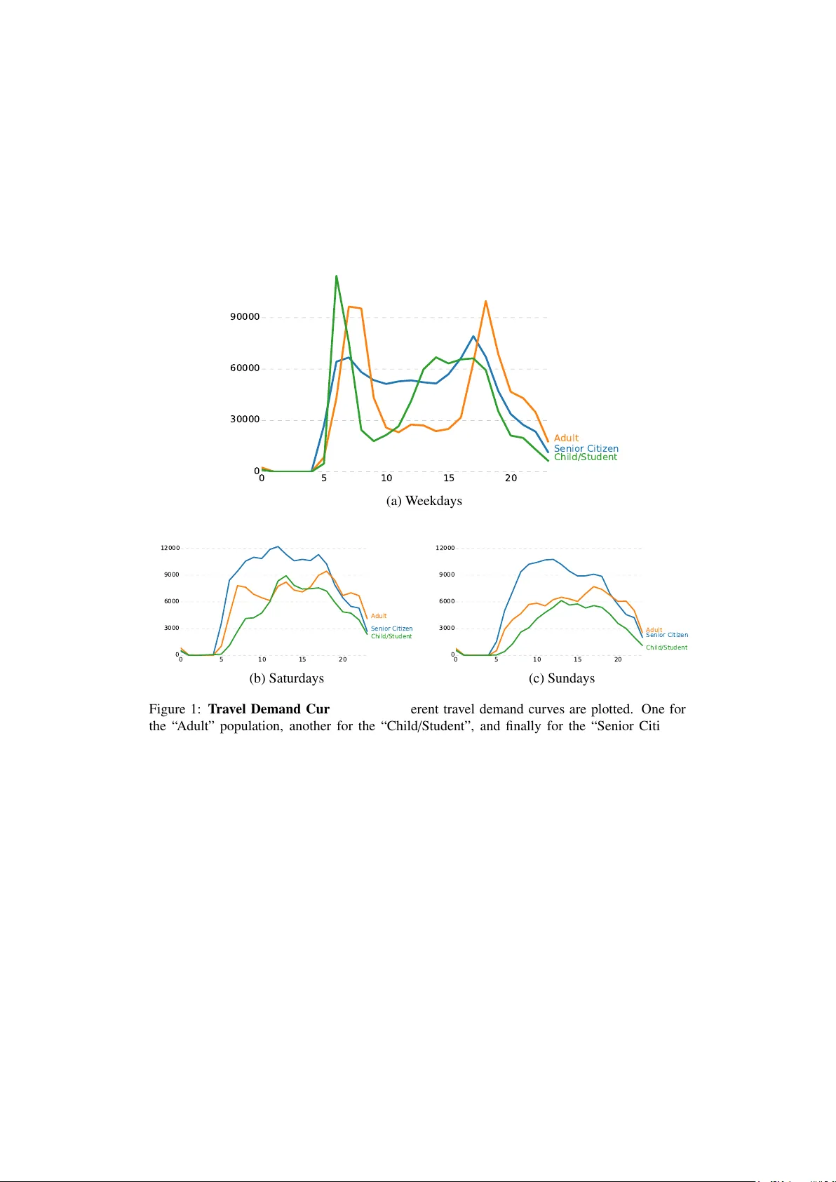
Inferring Passenger T ype from Commuter Eigentra vel Matrices E.F . Legara and C. Monterola Institute of High P erformance Computing, Agency for Science, T echnolo gy , and Resear c h, Singapor e 138632 Abstract A su ffi cient knowledge of the demographics of a commuting public is essential in formulating and implementing more targeted transportation policies, as commuters exhibit di ff erent ways of trav eling—including time in the day of travel, the duration of trav el, and ev en the choice of transport mode. W ith the advent of the Automated Fare Collection system (AFC), probing the tra vel patterns of commuters has become less in v asi ve and more accessible. Consequently , numerous transport studies related to human mobility have shown that these observed patterns allow one to pair individuals with locations and / or acti vities at certain times of the day . Howe v er , classifying commuters using their trav el signatures is yet to be thoroughly examined. Here, we contrib ute to the literature by demonstrating a procedure to characterize passen- ger types (Adult, Child / Student, and Senior Citizen) based on their three-month trav el patterns taken from a smart fare card system. W e first establish a method to construct distinct commuter matrices, which we refer to as eigentravel matrices, that capture the characteristic trav el rou- tines of individuals. From the eigentravel matrices, we build classification models that predict the type of passengers trav eling. Among the models explored, the gradient boosting method (GBM) gi ves the best prediction accuracy at 76%, which is 84% better than the minimum model accuracy (41%) required vis- ` a-vis the proportional chance criterion. In addition, we find that trav el features generated during weekdays have greater predicti ve po wer than those on week- ends. This work should not only be useful for transport planners, but for market researchers as well. W ith the awareness of which commuter types are traveling, ads, service announcements, and surv eys, among others, can be made more targeted spatiotemporally . Finally , our frame work should be e ff ective in creating synthetic populations for use in real-world simulations that in volv e a metropolitan’ s public transport system. K e ywor ds: T ransport, Human mobility, Acti vity pattern recognition, Commuter classification, Automated fare collection, Sociodemographics, Machine learning, Gradient boosting method, Random forest 1. Introduction The era of big and smart data has provided a substantial impetus in understanding human mobility—rev ealing the regularity and predictability of human behavior . In transport studies in particular , the widespread use of contactless smart fare card systems has spurred considerable growth in the field [1, 2, 3, 4, 5]. The main focus of most disquisitions on human mobility has Pr eprint submitted to Elsevier September 12, 2018 been on identifying and / or predicting activity locations giv en an indi vidual’ s past transportation transactions record, essentially spotting places where an individual goes to and hangs around at certain times of day—rev ealing ones home, work, and “third place” [6, 7, 8, 9, 10, 11]. Understanding human mobility is especially consequential in urban land-use and transporta- tion planning [12, 13]. Gaining insights on where people go and what acti vities the y engage in, or ev en inferring what dri ves them to travel from one place to another, can help in designing smart cities that can su ffi ciently address the needs of their citizens from their environment [14, 15]; thereby improving their o verall well-being. Notwithstanding the fact that most human mobility studies are centered on matching indi- viduals with locations and / or activities, certain sociotechnical datasets hav e more to o ff er other than spatial information. In this study , for example, we utilize data from travel fare cards that not only have spatiotemporal information such as origin, destination, time of trav el, and duration of travel, but also provide a particular demographic information, which is the type of passenger trav eling, i.e. Adult, Child / Student, or Senior Citizen. In this work, instead of predicting where people go at certain times of the day , we determine a set of features based on trav el routines that can help identify which passenger types are trav eling. Realizing commuter types can give us a better understanding of the structure of a society and the needs of its people from their surroundings. From the perspecti ve of transport planning, this can help stakeholders quantify more systematically how a certain group of commuters would react to or be a ff ected by changes in the entire transport system—from infrastructure changes to policy changes [14, 16]. Finally , from the standpoint of modeling and simulations, our proposed approach can aid in setting up synthetic populations wherein di ff erent passenger categories e xhibit v arying trav el signatures. The paper is organized as follo ws. In the next section, we discuss the data used in the study . This is then follo wed by a methods section where (1) present some descriptiv e statistics rele v ant to the construction of our classification models, and (2) demonstrate in detail how we set up the eigentrav el matrices that define the feature variables used in building the classification models. Finally , we end the article with a discussion and conclusion section where we elaborate on our results and share some insights into them. 2. Data This paper looks into movements of public transport commuters within Singapore using a three-month travel dataset. In the city-state, there is only one smart fare card system called EZ- link used in both its b us and rail transit system (R TS). Moreover , the public transport system has both entry and exit automated fare collection (AFC) for the bus and R TS. With both entry and exit AFC, the durations of travel for each transaction can be ev aluated in a straightforward manner . The dataset at hand has more than 3 million unique and anonymized card ID’ s; this includes single journe y transactions across the three months under study . For purpose of computation, we utilized a randomly sampled population of 30,000 r e gular commuters. Such sampling yields a confidence interval equal to 99.99% or an error of less than 0.01%. The population is equally split among three passenger types: adult, child / student, senior citizen. Each travel transaction contains the follo wing pieces of information that are rele vant to the study: card ID, origin, destination, start date (of travel), start time (of tra vel), end time (of travel), mode of transport (bus or rail), and passenger type. 2 3. Methodology 3.1. Descriptive Statistics 0 5 10 15 20 0 30000 60000 90000 Senior Citizen Adult Child/Student (a) W eekdays 0 5 10 15 20 0 3000 6000 9000 12000 Senior Citizen Adult Child/Student 0 5 10 15 20 0 3000 6000 9000 12000 Senior Citizen Adult Child/Student (b) Saturdays (c) Sundays Figure 1: T rav el Demand Curve . Three di ff erent travel demand curves are plotted. One for the “ Adult” population, another for the “Child / Student”, and finally for the “Senior Citizen” population. The “ Adult” demand curve displays the typical demand curves that are discussed in the transportation research literature wherein there are two distinct peaks—one for the morning peak hours and another for the evening peak hours. On the other hand, the “Child / Student” demand curve only exhibits one well-defined peak. Finally , the “Senior Citizen” curve displays no distinquishable peak, but instead a plataeu suggesting that senior citizens typically do not follow a “univ ersal” routine wherein they go to work in the mornings and go home from work in the ev enings. W e first look at some descriptiv e statistics that can be derived from the dataset. In Fig. 1, we show the temporal travel demand statistics via the ride start time distributions for each pas- senger type. A typical weekday trav el demand curve that we see in the literature is that there are two distinct peaks that correspond to both the AM and PM peak hours— when people go to work / school (in the morning) and when they go home (in the afternoon) [3, 5]. Howe ver , when we discriminate across passenger types, we see three distinct curves (Fig. 1a). The curve for the passenger type “ Adult” ( A -curve) is the same as the usual travel demand curves presented in the 3 Adult Senior Child/Student 0 150000 300000 450000 600000 750000 Bus RTS (a) W eekdays Adult Senior Child/Student 0 25000 50000 75000 100000 125000 Bus RTS Adult Senior Child/Student 0 25000 50000 75000 100000 Bus RTS (b) Saturdays (c) Sundays Figure 2: Mode of T ransport . For the three subplots (a), (b), and (c), the travel mode distribu- tions for three types of passenger population are shown. Except for the drop in the ridership on weekends, the mode trends are quite consistent across the week, i.e. the bus ridership dominates the R TS. The dominance is especially evident for the “Senior” population were more than 50% ov er the total trips utilize the bus system. The “ Adult” population utilizes the R TS more often than the other two. literature. Howe ver , for the trav el demand curve of children / students ( C -curve), we see that there is only one sharp peak that is found in the morning; in the afternoon, the curve plateaus. This suggests that children / students have practically v arying end-of-school times—spread from 1300 hours to 1800 hours as there are students who only go to class in the morning. Finally , the travel demand curve for the elderlies (senior citizen, S -curve) does not reveal a peak, which implies that seniors typically do not have a “univ ersal” schedule. These three demand curves give a hint on how to set up the di ff erent tra vel features for classifying passenger types. W e probe these curves in greater detail in the Results and Discussion section below . W e also look at how the two modes of Singapore public transport, bus and train, are utilized across the period under study for the three types ( see Figure 2). The barplots show that, in general, the usage of bus dominates that of the rail. This is more pronounced for the elderlies wherein around x % of the total trips account for the bus usage. 4 Figure 3: Eigentravel Matrix B : Schematic Diagram . The eigentrav el matrix B is a 42 × 20 matrix. The entire dataset cov ers a total of fourteen (14) weeks. W e then separate the weekdays from the weekends, and further distinguish between saturdays and sundays. The first fourteen rows are for the fourteen weeks for the weekdays, while the last two fourteen-week slabs, for saturdays and sundays. Each ro w is referred to as a w -slice or a week-slice. The twenty columns, on the other hand, represent each hour from 0400 hours to 2359 hours of each day . Each cell or hour slice in a w -slice is referred to as one h -slice. For the first fourteen rows, the characteristic trav el patterns are averaged across the weekdays of each week. Finally , each b w , h cell has a v alue that ranges from 0 to 10. Details are discussed in Fig. 4. 14 weeks W eekdays Saturdays Sundays 42 weeks 20 hours 3.2. Eigentravel Matrices Building from what have been established in the pre vious section, we construct a unique eigentrav el matrix B i for each agent i to characterize an individual’ s travelprint. B i captures, at the minimum, the observed di ff erences in trav el demand (or ride times) of each passenger type and their preferred modes of transport. B i is a two-dimensional 42 × 20 matrix. The forty-two (42) rows correspond to three 14- week partitions from the three-month data. The first fourteen rows aim to capture the trav el patterns on weekdays; while the second and third fourteen-week slabs correspond to saturdays and sundays, respecti vely . In this study , only trips between 0400 and 2359 hours of each day are captured— this is depicted in the 20 columns that represent each hour of the time period under study . Figure 3 shows a schematic diagram of an individual i ’ s B i -matrix. In Figure 4, we zoom in on one of the forty-two week slices in B i . The figure is discussed in greater detail belo w . Meanwhile, the eigentrav el matrix B i is constructed to not only quantify when an agent is 5 Figure 4: w -slice: Eigentravel Pattern for a W eek Slice. Each row in matrix B are divided into 20 h -slices corresponding to each hour from 0400 hours to 2359 hours. Each h -slice is further divided into 60 m -slices or minute slices. In this figure, we illustrate how a set of trav el transactions of an individual as shown in T able 1 is represented in B . Journey 1 in volv es a total of ∆ ρ = 12 minutes of tra vel by bus from 0651 to 0702 hours. For Journey 1, h -slices 3 and 4 are partially shaded accrodingly (with blue for the bus tra vel mode)—a total of 9 m -slices for h = 3, and 2 m -slices for h = 4. Similarly , for Journey 2, h -slices 15 and 16 are partially shaded (red for the use of the R TS) cov ering 18 m -slices and 17 m -slices, respectively . Finally , for Journey 3, ∆ ρ = 6 m -slices are shaded in h = 16 for the bus trip from 1953 hours to 1959 hours. Note that since the focus of the study is from 0400 hours, h = 1 correspond to 4:00 AM, h = 2 to 5:00 AM, and so on. m -slice (1min) h -slice (1hr) 1 2 3 4 4 AM 12 Midnight 12 Noon … 6 PM 0 60 51 … 0 60 2 h = 3 h = 4 … 0 60 42 … 0 17 h = 15 h = 16 59 53 15 16 Δρ = 9 Δρ = 18 Δρ = 17 Δρ = 6 17 18 19 20 trav eling, but to also carry information on a commuter’ s transport mode of choice and his / her durations of trav el. Each cell b w , h in B i can hav e a value in the range [0 , 10] and is giv en by 6 b w , h = P j ∈ J h w f ∆ ρ 60        f = 1 , bus f = 10 , train (1) where j = 1 , 2 , ... is a journey in the journey set J h w , which is a collection of all journeys that begin on week w at hour h 0 and ends on the same week and day at hour h f where h f ≥ h 0 . ∆ ρ , on the other hand, is the duration of travel (in minutes) of the indi vidual in week w and hour h . If a journey cov ers two adjacent hours, say the travel was from 0651 hours to 0702 hours covering hours 0600 ( h = 3) and 0700 ( h = 4), respectively , the corresponding travel duration for each hour will be counted separately . Finally , to distinguish between using a bus and a rail transit, a multiplier f of either 1.0 or 10.0 is introduced. T able 1: Sample travel transactions of a commuter . The table shows three hypothetical jour- neys taken by a commuter . W e use this to illustrate how we build an individual’ s eigentravel matrix. The table entries are “visualized’ in Figure 4 . Jour ney Start Date Start Time End Time T rav el Mode Passenger T ype 1 Monday , W eek 1 6:51 AM 7:02 AM Bus Adult 2 Monday , W eek 1 6:42 PM 7:17 PM R TS Adult 3 Monday , W eek 1 7:53 PM 7:59 PM Bus Adult T o illustrate the construction of B i , consider the tra vel transactions of a hypothetical agent in T able 1. In Journeys 1 and 3, the agent utilized the b us system; therefore, f = 1 for the two trips. For Journey 2, on the other hand, the factor f = 10 since the agent utilized the rail transit system (R TS). For Journey 1, the trip crosses two h -slices— h = 3 and 4, respectively (see Fig. 4). Note that in this study , we are starting at 0400 hours ( h = 1), therefore, h = 3 and h = 4 for 6AM and 7AM, respectiv ely . In Fig. 4, we can see that Journey 1 cov ers a duration of ∆ ρ = 9 mins and ∆ ρ = 2 mins for h = 3 and h = 4, respectively . Consequently , cells b 1 , 3 and b 1 , 4 of B i will hav e non-zero values, and are computed as follows: b 1 , 3 = 1 × 9 60 and b 1 , 4 = 1 × 2 60 . From Journey 2, b 1 , 15 = 10 × 18 60 . Finally , from Journeys 2 and 3, b 1 , 16 = (10 × 17) + (1 × 6) 60 . Actual samples of eigentravel matrices are shown in Figure 5. 3.3. Classification W e utilize di ff erent supervised machine learning models and perform predicti ve analytics on the constructed eigentrav el matrices. The three best models are (1) a distributed random forest (DRF) model, (2) a gradient boosting method (GBM), and (3) a support vector machine (SVM). These methods are standard advanced classification techniques in machine learning and have demonstrated success in a wide range of systems [17, 18, 19, 20]. Both DRF and GBM are forward-learning ensemble models made-up of multiple basis elements— the decision trees (DT) [18, 21, 22]. Each DT in each of the ensemble pro vides a “weak” solution to the classification problem at hand. The main di ff erence between DRF and GBM lies in how the two models generate their base models. In the DRF , the individual DTs are generated indepe- dently , and the fitting simply averages the performance of each of the learners; in the GBM, on the other hand, a gradient-descent based boosting formulation with the objectiv e of minimizing the loss function in every iteration is implemented in spawning new learners. In spite of this, 7 Figure 5: Eigentrav el Matrices. Randomly sampled eigentravel matrices for illustration. Three samples for each passenger type (one per row). Adult Child or Student Senior Citizen Hour W eek Numbe r similar to DRF , the final fitting is just the average of the base models. Finally , SVM is a super- vised classification technique where sample clusters are separated by defining hyperplanes that giv e the largest minimum distances from each cluster . The forward-learning ensemble models DRF and GBM are implemented using the H2O Python Module [23], while the SVM is performed using scikit-learn [24]—a machine learn- ing Python module. W e note that linear models and deep learning methods produce results that are inferior when compared to the methods described abov e. 8 3.4. F eatur es W e reshape each of the eigentrav el matrices into one-dimendional arrays whose elements correspond to the 42 × 20 = 840 features considered in this study . The features contain infor- mation on the trav el time of the individuals and their preferred mode of transport as described in Section 3.2. The predictor variables are labelled F 1 , F 2 , ..., F 840, where F 1 corresponds to the average ride pattern of an individual during weekdays for the first week under consideration at 0400 hours. F 2, on the other hand, is for the same week averaged across weekdays at 0500 hours. Finally , F 400 is the 5th Saturday in the data set at 2400 hours. The response variable is the passenger type . 4. Results and Discussion W e compare our results for each of the models by comparing their accuracy rates against the proportional chance criterion (PCC)—a common yardstick in ev aluating the success of a classifier when compared to a random chance prediction [25]. PCC is calculated by summing the squared proportion of each of the group represented in the sample. As a rule of thumb, a successful model, indicati ve of a significant predicti ve score, should ha ve an accurac y of at least 25% of the PCC [26]. Accordingly , our objecti ve is to hav e an accurac y of at least PCC × 1 . 25 = [( 75 225 ) 2 ∗ 3] × 1 . 25 = 0 . 4125. Figure 6: V ariable Importance Heat Maps . The 1 (bottom) to 42 (top) ro ws represent the week number (1-14 for weekdays, 15-28 for saturdays, and 29-42 for sundays) while the columns rep- resent the 20 hours under consideration. The boxed portions of the maps highlight the variables associated with weekday trav els. 1 2 3 4 5 6 7 8 9 10 11 12 13 14 15 16 17 18 19 20 1 2 3 4 5 6 7 8 9 10 11 12 13 14 15 16 17 18 19 20 21 22 23 24 25 26 27 28 29 30 31 32 33 34 35 36 37 38 39 40 41 42 1 2 3 4 5 6 7 8 9 10 11 12 13 14 15 16 17 18 19 20 1 2 3 4 5 6 7 8 9 10 11 12 13 14 15 16 17 18 19 20 21 22 23 24 25 26 27 28 29 30 31 32 33 34 35 36 37 38 39 40 41 42 DRF GBM T ime of Day (Hours) W eek Number Among the three models, GBM resulted to the highest prediction accuracy of 76%, which is 84% better than the minimum required model accuracy (41%) deriv ed from the PCC. DRF and SVM gave 72% and 64% accuracy rates, respectively . The deep learning method we performed with layers sampled from 1 to 200 and hidden nodes from 100 to 600 only reached a maximum of 64%, while results from the linear methods are just within 1 . 25 × P C C . Focusing on both GBM and DRF , which resulted to greater than 70% accuracy rates, we provide heatmaps of the scaled v ariable importances (see Figure 6). What is apparent in the 9 Figure 7: Mean Scaled V ariable Importance Across W eekdays . The plot sho ws the av erage scaled variable importance for each hour across weekdays. T wo methods are highlighted here- with: distributed random forest (DRF) and gradient boosting machine (GBM). What can be seen here is that for the GBM, the hours 0600, 1100, 1400, and 1500 dominate the other predictor variables; for the DRF , on the other hand, hours 0800, 1100, 1400, and 1500 go vern the others. ● ● ● ● ● ● ● ● ● ● ● ● ● ● ● ● ● ● ● ● ● ● ● ● ● ● ● ● ● ● ● ● ● ● ● ● ● ● ● ● 0.0 0.1 0.2 0.3 5 10 15 20 Time of Day (Hours) Scaled V ar iable Importance model ● ● DRF GBM figure is that most of the variables associated with the trips made during weekdays (boxed slabs) dominate the rest of the features; that is, the predictor v ariables corresponding to weekend travels do not contribute significantly in identifying passenger clusters. This finding concurs with the trav el demand curves shown in Fig. 1 where the ov erall profiles of the curves for the three types for both Saturdays (Fig. 1b) and Sundays (Fig. 1c) are structurally similar . In Fig. 7, we zoom in on the weekdays of the fourteen weeks by taking the av erage of the scaled variable importances of features that represent the same hour of the weekdays. In the plot, for the GBM, the leading v ariables are those identified with the hours: 0600, 1100, 1400, and 1500; for the DRF , the prominent variables are those at 0800, 1100, 1400, and 1500. T able 2: Confusion Matrix . This is the confusion matrix generated by the GBM. In the matrix, it is apparent that predicting children / students giv es the highest accuracy ,with only an error rate of approximately 15.4%, compared to when predicting the adults and / or senior citizens. The model utilized shows di ffi culty in distinguishing between an adult and a senior citizen. Adult Child Senior Error Rate Adult 3637 392 971 27.3% 1,363 / 5,000 Child 497 4223 280 15.4% 777 / 5,000 Senior 1175 379 3444 31.09% 1,554 / 4,998 T otal 5,309 4,994 4,695 24.6% 3,694 / 14,998 10 The variable importance values may be explained by looking at Fig. 1 and T able 2, which shows a sample confusion matrix resulting from implementing the GBM. T able 2 establishes that predicting children and / or students giv es the highest accuracy with only an error rate of approx- imately 17.4%; compared to the adults and senior citizens where the error rates are 28.5% and 34.4%, respectively . In addition, most of the misclassification are between the adults and senior citizens; therefore, we reckon that predictor variables that maximize the dissimilarity between the adults and senior citizens will play more significant roles in the models. W e now discuss what insights we can deriv e from the tra vel patterns of the commuters, focus- ing on the sets of the most relev ant predictor variables. For ease of discussion, we introduce v h to represent a set of 14 weekday predictor v ariables that fall under a gi ven hour ( h = 1 , 2 , ..., 20). T o recap, from Section 3.2, h = 1 refers to 0400 hours, h = 2 to 0500 hours, and h = 19 to 2200 hours. T o illustrate further , v h = 1 = { F 1 , F 21 , F 41 , ..., F 261 } , which is a set of 14 (weekday) vari- ables that fall within the first hour of each weekday considered. From the variable importance results for the GBM and DRF , we focus on the sets G = { v 3 , v 8 , v 11 , v 12 } and D = { v 5 , v 8 , v 11 , v 12 } , respectiv ely; these sets refer to v ariables under the follo wing time frames: 0600, 1100, 1400, and 1500 hours for the GBM and 0800, 1100, 1400, and 1500 hours for the DRF . In Section 3.1, the general profiles of the di ff erent trav el demand curves in Fig. 1 for the adults ( A -curv e), the children / students ( C -curve), and the senior citizens ( S -curve) are discussed. W e look into specific se gments of the curves guided by the sets G and D . Note that each variable set v h in either of the sets isolates one particular curve from the rest of the curves. This is intuitiv e since the best predictors maximize the dissimilarity between curves. First, we take a look at v 3 ∈ G (at 0600 hours) where the C -curve is at its highest and narrowest (also when compared against the two other curves). At this hour , almost all children commuters are on their w ay to school. The narro wness of the C -curve peak implies that the start time of schools are highly likely the same across the city-state and that they are more rigid than the adult working hours—the A -curve within the same time frame is wider . In addition, at 0600 hours, the C -curve is isolated from the intersecting A and S -curves. Almost similar dynamics is surmised for v 5 ∈ D ; howe ver , the C -curve peak has started to drop at lower travel demand lev els. Second, we focus on v 8 ∈ G , D at 1100 hours. At 1100 hours, both the students / children and the working adult population are in their schools / o ffi ces; that is, they are not traveling. This may explain why both A and C -curves at that hour are overlapping—isolating the S -curve. In addition, notice that in Fig. 1a, the S -curve has no prominent peak unlike in the A -curv e (2 peaks) and C -curve (1 peak). This is not surprising since most senior citizens do not follow “regular” adult working hours (although some may still do as depicted by the tw o shallow “bumps” around the same region where the A -curve peaks). It can be said that, by and large, the elderlies do not hav e a “universal” schedule unlike the working adults, and that during “working hours” when the students and working adults are at work or in school, more elderlies are trav eling. Finally , for v 11 and v 12 ∈ G , D , at 1400-1500 hours, the A -curve is left at the lower lev els of the travel demand and is isolated from the C and S -curves. This is a particularly interesting trend for the student / child population, which rev eals that most students are only in schools for half a day and that they hav e varying end of school times. This is manifested in the C -curve where there is no second peak observed as it starts to plateau at 1300 to 1800 hours. In addition, from 1400-1500 hours, the trav el demand curve implies that most working adults are still in their o ffi ces. The insights presented here are summarized in T able 3. 11 T able 3: T op Predictor V ariables . W e highlight the top predictor variables in terms of their variable importance v alues. It can be seen that for each predictor v ariable, a tra vel demand curv e is isolated from the rest. Furthermore, all curves are, in one way or another , well-represented in the choice of feature variables. Predictor Hour of Day Isolated Curv e Remarks v 3 v 5 0600 hours 0800 hours C -Curve Students / children dominate trav el demand T ravel demand highest and narro west v 8 1100 hours S -Curve W orking adults in o ffi ces Children / students in classes Senior citizens trav eling v 11 v 12 1400 hours 1500 hours A -Curve W orking adults in o ffi ces Senior citizens trav eling Students / children trav eling home 5. Conclusion A su ffi cient knowledge of the demographics of a commuting public is essential in formulating and implementing more targeted transportation policies—di ff erent schemes can a ff ect di ff erent commuter types in several ways. In this work, using data taken from Singapore’ s automated fare collection (AFC) system, we sho wed that commuters e xhibit varying travel patterns that can be used to categorize passengers into three general types: adult, child / student, senior citizen. W e first established a method to construct distinct commuter matrices that we referred to as eigentravel matrices that capture the characteristic travel routines of indi viduals by taking into account their times in the day of travel, durations of travel, and preferred modes of transport. W e then performed a multiv ariate analysis (840 feature variables) on the eigentravel matrices using three supervised machine learning models: gradient boosting method (GBM), distributed random forest (DRF), and support v ector mahine (SVM). GBM ga ve the best prediction accuracy of 76%. Furthermore, implementing a variable importance analysis showed that features associated with weekday trav els are better than those associated with weekends. Many cities are already using AFC systems, and some metropolitan areas in the dev eloping worlds are already transitioning into using such technology . Ho wever , not all AFC systems provide passenger type information like what the dataset in this study provides. Nev ertheless, with the approach presented, urban planners can now have a way to determine passenger types by looking at the “natural tendencies” of public transport commuters, thru eigentravel matrices, in a non-in vasi ve manner . The technique demonstrated allo ws transport planners to formulate more targeted transporta- tion policies and schemes. The framew ork is not only useful to urban and transport planners; the field of mark eting research may also find this work relev ant and beneficial. W ith adequate a ware- ness of which passenger types dominate the travel demand at specific times of day , ad agencies (and survey firms) can create andt put up more focused advertisements, service announcements, and surve ys—helping stakeholders to properly channel their resources. Finally , from the per- spectiv e of modeling and simulations, the categorization presented can be useful in generating synthetic populations for use as inputs to computational models (e.g. agent-based models) to accurately capture the rev ealed travel signatures for each commuter cate gory . 12 Acknowledgement W e would like to thank the Land T ransport Authority of Singapore for the ticketing data used in this work, Nasri bin Othman for his assistance in preparing the datasets, and Hu Nan for his valuable feedback on the work. This research is supported by Singapore A ∗ SERC Complex Systems Programme research grant (1224504056). References [1] X. Ma, Y .-J. W u, Y . W ang, F . Chen, J. Liu, Mining smart card data for transit riders’ travel patterns, Transportation Research Part C: Emer ging T echnologies 36 (2013) 1–12. [2] S. G. Lee, M. D. Hickman, Trav el pattern analysis using smart card data of regular users, in: Proceedings of the 90th T ransportation Research Board Annual Meeting, 11-4258, 2011. [3] L. Sun, D.-H. Lee, A. Erath, X. Huang, Using smart card data to extract passenger’ s spatio-temporal density and train’ s trajectory of mrt system, in: Proceedings of the A CM SIGKDD International Conference on Knowledge Discovery and Data Mining, 2012. [4] A. Chakirov , A. Erath, Use of public transport smart card fare payment data for travel behaviour analysis in singa- pore, in: 16th International Conference of Hong K ong Society for Transportation Studies, Hong K ong, 2011. [5] E. F . Legara, K. K. Lee, G. G. Hung, C. Monterola, Mechanism-based model of a mass rapid transit system: A perspectiv e, in: International Journal of Modern Physics Conference, no. 1560011 in 36, 2015. [6] O. J ¨ arv , R. Ahas, F . Witlox, Understanding monthly variability in human activity spaces: A twelve-month study using mobile phone call detail records, Transportation Research Part C: Emerging T echnologies 38 (2014) 122–135. [7] T . Kusakabe, Y . Asakura, Behavioural data mining of transit smart card data: A data fusion approach, Transporta- tion Research Part C: Emer ging T echnologies 46 (2014) 179–191. [8] M.-P . Pelletier , M. T r ´ epanier , C. Morency , Smart card data use in public transit: A literature revie w , Transportation Research Part C: Emer ging T echnologies 19 (4) (2011) 557–568. [9] K. G. Goulias, Longitudinal analysis of acti vity and trav el pattern dynamics using generalized mix ed mark ov latent class models, T ransportation Research Part B: Methodological 33 (8) (1999) 535–558. [10] N. Nassir , M. Hickman, Z. Ma, Activity detection and transfer identification for public transit fare card data, T ransportation 42 (2015) 683–705. [11] S. G. Lee, M. D. Hickman, Trip purpose inference using automated fare collection data, Public Transport 6 (1-2) (2014) 1–20. [12] K. K. A. Chu, R. Chapleau, Enriching archi ved smart card transaction data for transit demand modeling, in: T rans- portation Research Record: Journal of the T ransportation Research Board, no. 2063, 2008, pp. 63–72. [13] M. Utsunomiya, J. Attanucci, N. H. Wilson, Potential uses of transit smart card re gistration and transaction data to improve transit planning, in: Transportation Research Record: Journal of the Transportation Research Board, no. 1971, 2006, pp. 119–126. [14] S. A. O. Medina, A. Erath, Estimating dynamic workplace capacities by means of public transport smart card data and household travel survey in singapore, in: Transportation Research Record: Journal of the Transportation Research Board, V ol. 2344, 2014, pp. 20–30. [15] N. bin Othman, E. F . Legara, V . Selvam, C. Monterola, Simulating congestion dynamics of train rapid transit using smart card data, in: Procedia Computer Science, V ol. 29, 2014, pp. 1610–1620. [16] M. A. Ortega-T ong, Classification of london’s public transport users using smart card data, Master’ s thesis, Mas- sachusetts Institute of T echnology (June 2013). [17] V . Etter , M. Kafsi, E. Kazemi, Been there, done that: What your mobility traces reveal about your behavior, in: International Conference on Pervasi ve Computing: Mobile Data Challenge, 2012. [18] Y . Zhang, A. Haghani, A gradient boosting method to improv e travel time prediction, T ransportation Research P art C: Emerging T echnologies. [19] T . Hastie, R. Tibshirani, J. Friedman, The Elements of Statistical Learning: Data Mining, Inference, and Prediction, second edition Edition, Springer , 2009. [20] G. Leshem, Y . Ritov , Tra ffi c flow prediction using adaboost algorithm with random forests as a weak learner, International Journal of Intelligent T echnology 2 (2) (2007) 111–116. [21] J. H. Friedman, Greedy function approximation: A gradient boosting machine, The Annals of Statistics 29 (5) (2001) 1189–1232. [22] C. Click, J. Lanford, M. Malohlava, V . Parmar , Gradient Boosted Models with H2O’ s R Package, 2nd Edition, H2O.ai, Inc., 2307 Leghorn Street Mountain V iew , CA 94043, 2015. [23] H. C. T eam [online] (2015) [cited 20 August 2015]. [link]. 13 [24] F . Pedregosa, G. V aroquaux, A. Gramfort, V . Michel, B. Thirion, O. Grisel, M. Blondel, P . Prettenhofer, R. W eiss, V . Dubourg, J. V anderplas, A. Passos, D. Cournapeau, M. Brucher , M. Perrot, ´ E. Duchesnay , Scikit-learn: Machine learning in python, Journal of Machine Learning Research 12 (2011) 2825–2830. [25] E. F . Legara, C. Abundo, C. Monterola, Ranking of predictor variables based on e ff ect-size criterion provides an accurate means of automatically classifying opinion column articles, Physica A: Statistical Mechanics and Its Applications 390 (1) (2011) 110–119. [26] J. F . H. Jr, W . C. Black, B. J. Babin, R. E. Anderson, Multi variate Data Analysis, sev enth Edition, Prentice Hall, 2009. 14