Enhancement and Recognition of Reverberant and Noisy Speech by Extending Its Coherence

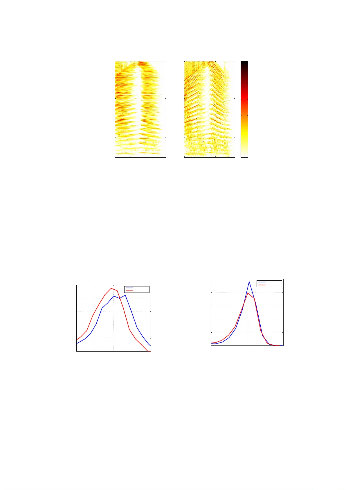
Enhancemen t and Recognition of Rev erb eran t and Noisy Sp eec h b y Extending Its Coherence Scott Wisdom ∗ 1 , Thomas P ow ers 1 , Les A tlas 1 , and James Pitton 1,2 1 Departmen t of Electrical Engineering, Universit y of W ashington 2 Applied Ph ysics Lab oratory , Universit y of W ashington Septem b er 3, 2015 Abstract Most sp eec h enhancement algorithms mak e use of the short-time F ourier transform (STFT), which is a simple and ﬂexible time-frequency decomposition that estimates the short-time spectrum of a signal. Ho wev er, the duration of short STFT frames are inher- en tly limited b y the nonstationarity of sp eech signals. The main contribution of this pap er is a demonstration of speech enhancemen t and automatic speech recognition in the presence of reverberation and noise by extending the length of analysis windo ws. W e accomplish this extension b y p erforming enhancement in the short-time fan-chirp transform (STFChT) do- main, an ov ercomplete time-frequency representation that is coheren t with sp eec h signals o ver longer analysis window durations than the STFT. This extended coherence is gained b y using a linear model of fundamental frequency v ariation of v oiced sp eec h signals. Our approac h cen ters around using a single-channel minim um mean-square error log-sp ectral amplitude (MMSE-LSA) estimator prop osed b y Hab ets, which scales co eﬃcients in a time- frequency domain to suppress noise and reverberation. In the case of multiple microphones, w e prepro cess the data with either a minimum v ariance distortionless resp onse (MVDR) b eamformer, or a dela y-and-sum b eamformer (DSB). W e ev aluate our algorithm on both sp eec h enhancemen t and recognition tasks for the REVERB challenge dataset. Compared to the same pro cessing done in the STFT domain, our approach achiev es signiﬁcant improv e- men t in terms of ob jectiv e enhancement metrics (including PESQ—the ITU-T standard measuremen t for sp eec h qualit y). In terms of automatic sp eec h recognition (ASR) p erfor- mance as measured b y w ord error rate (WER), our exp erimen ts indicate that the STFT with a long window is more eﬀective for ASR. 1 In tro duction Enhancemen t and recognition of sp eec h signals in the presence of reverberation and noise remains a c hallenging problem in many applications. Many past metho ds are prone to generating artifacts in the enhanced sp eech, and must trade oﬀ noise reduction against sp eech distortion. Recen t approac hes ha ve started to address this issue, demonstrating impro vemen ts in b oth ob jectiv e sp eec h quality and automatic speech recognition [1, 2]. In this pap er, w e propose using a new time-frequency domain that is more coheren t with sp eec h signals ov er an extended p erio d of time, which allows longer analysis windo ws. In turn, longer analysis windows provide a more narrowband sp ectral representation, whic h concentrates signal energy into smaller num b ers of FFT bins. Within these bins, the signal-to-noise ratio (SNR) is increased, whic h results in less ov ersuppression of sp eec h. W e combine a statistically optimal single-c hannel enhancement algorithm that suppresses bac kground noise and reverber- ation with an adaptiv e time-frequency transform domain that is coherent with sp eech signals ∗ swisdom@uw.edu 1 o ver longer durations than the short-time F ourier transform (STFT). Th us, we are able to use longer analysis windows while still satisfying the assumptions of the optimal single-channel en- hancemen t ﬁlter. Multic hannel processing is made p ossible using a classic minim um v ariance distortionless resp onse (MVDR) b eamformer or, in the case of tw o-c hannel data, a delay-and-sum b eamformer (DSB) preceding the single-c hannel enhancemen t. First, w e review the speech enhancement and derev erb eration problem, as w ell as the en- hancemen t algorithm we use prop osed by Hab ets [3], whic h suppresses b oth noise and late rev erb eration based on a statistical mo del of reverberation (originally prop osed b y Lebart et al. [4]). Then, we describ e the fan-c hirp transform, proposed b y W eruaga and K ` ep esi [5, 6] and impro ved upon b y Cancela et al. [7], which pro vides an enhancement domain, the short-time fan-c hirp transform (STF ChT), that b etter matc hes time-v arying harmonic con ten t of v oiced sp eec h. W e discuss why performing the enhancement in the STF ChT domain gives sup erior results compared to the STFT domain. F urther impro vemen ts ov er our original submission [8] to the REVERB challenge [9] are describ ed, and w e explore more optimal parameter settings. W e presen t b oth speech enhancemen t and recognition results on the REVERB challenge dataset [9], which shows that our new metho d achiev es sup erior results versus con ven tional STFT-based pro cessing in terms of ob jective sp eec h enhancemen t measures. Through our automatic sp eec h recognition (ASR) experiments, we disco ver that STFT-based pro cessing with a longer window results in the low est w ord error rates. Th us, our algorithm is an example of an op eration that improv es enhancemen t and ob jectiv e quality metrics, but for reasons we h yp othesize the op eration does not improv e ASR. Ho w ever, our enhancement method ma y b e able to provide complemen tary features to conv entional STFT-based pro cessing. Our basic multic hannel (given multiple microphones) architecture of single-channel enhance- men t preceded b y beamforming is not unprecedented. Gannot and Cohen [10] used a similar arc hitecture for noise reduction that consists of a generalized sidelob e cancellation (GSC) b eam- former follo w ed by a single-c hannel post-ﬁlter. Maas et al. [11] emplo y ed a similar single-channel enhancemen t algorithm for rev erb eration suppression and observed promising sp eec h recognition p erformance in even highly reverberant environmen ts. There hav e b een several dereverberation and enhancement approaches that estimate and lev erage the time-v arying fundamental frequency f 0 of sp eec h. Nak atani et al. [12] prop osed a derev erb eration metho d using in verse ﬁltering that exploits the harmonicity of speech to build an adaptive comb ﬁlter. Kaw ahara et al. [13] used adaptiv e sp ectral analysis and estimates of f 0 to p erform manipulation of sp eec h characteristics. Dropp o and Acero [14] observed ho w the fundamental frequency of sp eec h can change within an analysis window, and prop osed a new framework that could b etter predict the energy of v oiced sp eec h. Dunn and Quatieri [15] used the fan-c hirp transform for sinusoidal analysis and synthesis of sp eec h, and Dunn et al. [16] also examined the eﬀect of v arious interpolation metho ds on reconstruction error. P antazis et al. [17] proposed an analysis/synthesis domain that uses estimates of instantaneous frequency to decomp ose sp eec h into quasi-harmonic AM- FM components. Degottex and Stylianou [18] prop osed another analysis/synthesis scheme for sp eec h using an adaptive harmonic mo del that they claim is more ﬂexible than the fan-chirp, as it allows nonlinear frequency tra jectories. Wisdom et al. show ed that the fan-chirp transform can b e used to build optimal detectors for nonstationary harmonics [19] and harmonically-mo dulated stationary pro cesses with time- v arying mo dulation frequency [20]. A preliminary version of this algorithm app eared in our REVERB c hallenge workshop pap er [8]. T o our kno wledge, these recent pap ers are the ﬁrst to use the fan-c hirp transform for statistical signal pro cessing. 2 Bac kground This section gives necessary background on single-c hannel suppression of noise and late rever- b eration and on the windo w duration- and hence coherence-extending fan-chirp transform. 2 2.1 Optimal single-c hannel suppression of noise and late rev erb eration In this section, we review the sp eec h enhancement problem and a p opular statistical sp eec h enhancemen t algorithm, the minimum mean-square error log-sp ectral amplitude (MMSE-LSA) estimator, whic h w as originally prop osed b y Ephraim and Malah [21, 22] and later improv ed b y Cohen [23]. W e review the application of MMSE-LSA to b oth noise reduction and joint derev erb eration and noise reduction. Joint derev erb eration and noise reduction was prop osed b y Habets [3]). 2.1.1 Noise reduction using MMSE-LSA A classic sp eec h enhancement algorithm is the minimum mean-square error (MMSE) short-time sp ectral amplitude estimator prop osed by Ephraim and Malah [21]. They later reﬁned the estimator to minimize the MSE of the log-sp ectra [22]. W e will refer to this algorithm as LSA (log-sp ectral amplitude). Minimizing the MSE of the log-sp ectra w as found to pro vide b etter enhanced output b ecause log-sp ectra are more p erceptually meaningful. Cohen [23] suggested impro vemen ts to Ephraim and Malah’s algorithm, whic h he referred to as “optimal mo diﬁed log-sp ectral amplitude” (OM-LSA). Giv en samples of a noisy sp eec h signal y [ n ] = s [ n ] + v [ n ] , (1) where s [ n ] is the clean sp eech signal and v [ n ] is additive noise, the goal of an enhancement algorithm is to estimate s [ n ] from the noisy observ ations y [ n ]. Clean sp eec h and noise are additiv e in the STFT domain: Y ( d, k ) = S ( d, k ) + V ( d, k ) . (2) The LSA estimator yields an estimate ˆ A ( d, k ) of the clean STFT magnitudes | S ( d, k ) | (where S ( d, k ) are assumed to hav e a prop er complex-v alued Gaussian distribution) by applying a frequency-dep enden t gain G LSA ( d, k ) to the noisy STFT magnitudes | Y ( d, k ) | : ˆ A ( d, k ) = G LSA ( d, k ) | Y ( d, k ) | . (3) Giv en these estimated magnitudes, the enhanced sp eec h is reconstructed from STFT co eﬃcien ts com bining ˆ A ( d, k ) with noisy phase: ˆ S ( d, k ) = ˆ A ( d, k ) e j ∠ Y ( d,k ) . (4) The LSA gains are computed as [22, equation (20)]: G LSA ( d, k ) = ξ ( d, k ) 1 + ξ ( d, k ) exp ( 1 2 Z ∞ v ( d,k ) e − t t dt ) . (5) The low er integral b ound in (5) is v ( d, k ) = ξ ( d, k ) 1 + ξ ( d, k ) γ ( d, k ) , (6) where ξ ( d, k ) and γ ( d, k ) are the a priori and a p osteriori signal-to-noise ratios (SNRs), resp ec- tiv ely , for the k th frequency bin of the d th frame. These SNRs are deﬁned to b e ξ ( d, k ) ∆ = λ s ( d, k ) λ v ( d, k ) and γ ( d, k ) ∆ = | Y ( d, k ) | 2 λ v ( d, k ) (7) where λ s ( d, k ) = E  | S ( d, k ) | 2  (8) end λ v ( d, k ) = E  | V ( d, k ) | 2  (9) 3 are the v ariances of S ( d, k ) and V ( d, k ), resp ectiv ely . Cohen [23] reﬁned Ephraim and Malah’s approach to include a lo w er bound G min for the gains as well as an a priori sp eec h presence probability (SPP) estimator p ( d, k ). Cohen’s estimator is as follows [23, equation (8)]: G OM − LSA = { G LSA ( d, k ) } p ( d,k ) · G 1 − p ( d,k ) min . (10) Cohen also derived an eﬃcient estimator for the SPP p ( d, k ) [23] that exploits the strong inter- frame and in terfrequency correlation of sp eec h in the STFT domain. 2.1.2 Join t derev erb eration and noise reduction This subsection reviews a MMSE-LSA enhancement algorithm prop osed by Hab ets [3] that uses a statistical mo del of reverberation to suppress b oth noise and late reverberation. Suc h a statistical mo del-based approac h to dereverberation was originally prop osed b y Lebart et al. [4]. W e will refer to this t yp e of MMSE-LSA as HMMSE-LSA (for Hab ets MMSE-LSA). The signal mo del Hab ets uses is y [ n ] = s [ n ] ∗ h [ n ] + v [ n ] = x e [ n ] + x ` [ n ] + v [ n ] , (11) where s [ n ] is the clean sp eech signal, h [ n ] is the ro om impulse response (RIR), and v [ n ] is additive noise. The terms x e [ n ] and x ` [ n ] corresp ond to the early and late reverberated sp eec h signals, resp ectiv ely . The partition b et ween early and late rev erb erations is determined by a parameter n e , which is a discrete sample index. All samples in the RIR b efore n e are taken to cause early reﬂections, and all samples after n e are taken to cause late reﬂections [3]. Thus, h [ n ] =      0 , if n < 0 h e [ n ] , if 0 ≤ n < n e h ` [ n ] if n e ≤ n. (12) Using these deﬁnitions, x e [ n ] = s [ n ] ∗ h e [ n ] and x ` [ n ] = s [ n ] ∗ h ` [ n ]. Hab ets prop osed a generalized statistical mo del of reverberation that is v alid b oth when the source-microphone distance is less than or greater than the critical distance [3]. This mo del divides the RIR h [ n ] in to a direct-path component h d [ n ] and rev erb eran t comp onen t h r [ n ]. Both direct-path and reverberant comp onen ts are taken to b e white, zero-mean, stationary Gaussian noise sequences b d [ n ] and b r [ n ] with v ariances σ 2 d and σ 2 r scaled by an exp onen tial deca y , h d [ n ] = b d [ n ] e − ¯ ζ n and h r [ n ] = b r [ n ] e − ¯ ζ n , (13) where ¯ ζ is related to the rev erb eration time T 60 b y [3]: ¯ ζ = 3 ln(10) T 60 f s . (14) Using this model, the exp ected v alue of the energy env elop e of h [ n ] is E  h 2 [ n ]  =      σ 2 d e − 2 ¯ ζ n , for 0 ≤ n < n d σ 2 r e − 2 ¯ ζ n , for n ≥ n d 0 otherwise, (15) where n d is a parameter chosen to be the num b er of samples that corresp ond to the direct part of a rev erb eran t signal. Figure 1 sho ws a schematic illustration of this statistical model of reverberation. Under the assumption that the sp eech signal is stationary ov er short analysis windows (i.e., duration muc h less than T 60 ), Hab ets prop osed [3, equation (3.87)] the following mo del of the spectral v ariance of the rev erb eran t comp onent x r [ n ], which is denoted by λ x r ( d, k ): λ x r ( d, k ) = e − 2 ¯ ζ ( k ) R λ x r ( d − 1 , k ) ... + E r E d  1 − e − 2 ¯ ζ ( k ) R  λ x d ( d − 1 , k ) , (16) 4 /43 1 Statistical modeling of r everberation * *Polack 1988, Habets 2010 2. Beyond locally stationar y: impr oved enhancement h e [ n ] h ` [ n ] n e n d 0 e  2 ¯ ⇣ n N 60 = b f s · T 60 c h 2 [ n ] Figure 1: Rev erb eration mo del. A schematic illustration of the statistical reverberation mo del giv en b y equations (12)-(15). where R is the n umber of samples separating t wo adjacent analysis frames and E r /E d is the in verse of the direct-to-reverberant ratio (DRR). The quantities E r and E d are the energies of the rev erb eran t and direct comp onen ts of the signal, respectively . The DRR expresses the energy level of the direct signal referenced to the energy lev el of the rev erb eran t part. Th us, the sp ectral v ariance of the reverberant comp onent in the current frame d is composed of scaled copies of the spectral v ariance of the rev erb eration and the spectral v ariance of the direct-path signal from the previous frame d − 1. Using this mo del, the v ariance of the late rev erb erant comp onen t can be expressed as [3, equation (3.85)]: λ x ` ( d, k ) = e − 2 ¯ ζ ( k )( n e − R ) λ x r  d − n e R + 1 , k  , (17) whic h is quite useful in practice, b ecause the v ariance of the late-reverberant comp onen t can b e computed from the v ariance of the total rev erb erant comp onent. T o suppress b oth noise and late reverberation, the a priori and a p osteriori SNRs ξ ( d, k ) and γ ( d, k ) from the previous section b ecome a priori and a p osteriori signal-to-interference ratios (SIRs), given b y [3, equations (3.25-26)]: ξ ( d, k ) = λ x e ( d, k ) λ x ` ( d, k ) + λ v ( d, k ) (18) and γ ( d, k ) = | Y ( d, k ) | 2 λ x ` ( d, k ) + λ v ( d, k ) . (19) The gains are computed by plugging the SIRs in (18) and (19) in to (5) and (6). Habets suggested an additional c hange to (10), which makes G min time- and frequency-dep enden t. This is done b ecause the in terference of b oth noise and late reverberation is time-v arying. The mo diﬁcation is [3, equation (3.29)] G min ( d, k ) = G min ,x ` ˆ λ x ` ( d, k ) + G min ,v ˆ λ v ( d, k ) ˆ λ x ` ( d, k ) + ˆ λ v ( d, k ) . (20) Notice that tw o parameters in (14) and (16) are not kno wn a priori ; namely , T 60 and the DRR. These parameters must be blindly estimated from the data. F or T 60 estimation, L¨ ollmann et al. [24] prop ose a maxim um-lik eliho od algorithm, which w e found to be eﬀective. As for the DRR, Hab ets suggests an online adaptive pro cedure [3, § 3.7.2]. This adaptiv e pro cedure constrains the DRR b et ween 0 and 1 and assumes that the source is within the critical distance (i.e., the distance at whic h direct and rev erb eran t energy are equal). This assumption preven ts o verestimation of the rev erb eran t v ariance when the direct signal is active. 2.2 Analysis using the forw ard fan-chirp transform In this section, we review the forward short-time fan-c hirp transform (STFChT), which is used as the time-frequency analysis-synthesis domain for our enhancement algorithm. In section 2.3, w e describe our nov el metho d of inv erting the STF ChT. 5 W e adopt the fan-chirp transform formulation used by Cancela et al. [7]. The forward fan-c hirp transform is deﬁned as X ( f , α ) = Z x ( t ) φ 0 α ( t ) e − j 2 πf φ α ( t ) dt (21) where φ α ( t ) =  t + 1 2 αt 2  and φ 0 α ( t ) = 1 + αt . The v ariable α is an analysis chirp rate. The c hirp rate α is a normalized chirp rate; that is, if the total bandwidth s w ept is B Hertz ov er a time duration T seconds, then α = B T f . Using a change of v ariable τ = φ α ( t ), (21) can be written as the F ourier transform of a time-w arp ed signal: X ( f , α ) = Z ∞ −∞ x ( φ − 1 α ( τ )) e − j 2 πf τ dτ . (22) The short-time fan-chirp transform (STFChT) of x ( t ) is deﬁned as the fan-chirp transform of the d th short frame of x ( t ): X d ( f , ˆ α d ) = Z T w / 2 − T w / 2 w ( τ ) x d ( φ − 1 ˆ α d ( τ )) e − j 2 πf τ dτ (23) where w ( t ) is an analysis windo w, ˆ α d (giv en by (27)) is the analysis chirp rate for the d th frame, and x d ( t ) is the d th short frame of the input signal of duration T : x d ( t ) = ( x ( t − dT hop ) , − T / 2 ≤ t ≤ T / 2 0 , otherwise . (24) T is the duration of the pre-w arp ed short-time duration, T hop is the frame hop, T w is the p ost-w arp ed short-time duration, and w ( t ) is a T w -long analysis window. The analysis windo w is applied after time-w arping so as to a void warping of the windo w, whic h can cause unpredictable smearing of the F ourier transform. Implemen ting the fan-chirp transform as a time-warping follo wed b y a F ourier transform allo ws eﬃcient implementation, consisting simply as an interpolation of the signal follow ed by an FFT. In the implemen tation pro vided b y Cancela et al. [7], the in terpolation used in the forw ard fan-c hirp transform is linear. K ` ep esi and W eruaga [5] pro vide a metho d for determination of the analysis chirp rate α using the gathered log sp ectrum (GLogS). The GLogS is deﬁned as the harmonically-gathered log-magnitude sp ectrum: ρ ( f 0 , α ) = 1 N h N h X k =1 ln | X ( k f 0 , α ) | (25) where N h is the maximum num b er of harmonics that ﬁt within the analysis bandwidth. That is, N h = $ f s 2 f 0  1 + 1 2 | α | T w  % . (26) Cancela et al. [7] prop osed sev eral enhancements to the GLogS. First, they observed improv ed results by replacing ln | · | with ln (1 + γ |·| ). Cancela et al. note that this expression appro ximates a p -norm, with 0 < p < 1, where low er v alues of γ with γ ≥ 1 approach the 1-norm, while higher v alues approaches the 0-norm. Cancela et al. note that γ = 10 gav e go o d results for their application. Additionally , Cancela et al. prop ose mo diﬁcations that suppress multiples and subm ultiples of the current f 0 . Also, they prop ose normalizing the GLogS such that it has zero mean and unit v ariance. This is necessary b ecause the v ariance of the GLogS increases with increasing fundamen tal frequency . F or means and v ariances measured ov er all frames in a database, a p olynomial ﬁt is determined and the GLogS are comp ensated using these p olynomial ﬁts. Let ¯ ρ d ( f 0 , α ) b e the GLogS of the d th frame with these enhancemen ts applied. F or prac- tical implemen tation, ﬁnite sets A of candidate c hirp rates and F 0 of candidate fundamental 6 frequencies are used, and the GLogS is exhaustiv ely computed for ev ery c hirp rate in A and fundamen tal frequency in F 0 . The analysis c hirp rate ˆ α d for the d th frame is th us found b y ˆ α d = argmax α ∈A max f 0 ∈F 0 ¯ ρ d ( f 0 , α ) . (27) 2.3 Syn thesis using the in verse fan-c hirp transform In verting the fan-chirp transform is a matter of reversing the steps used in the forward trans- form. Th us, the inv erse fan-chirp transform for a short-time frame consists of an inv erse F ourier transform, remo v al of the analysis windo w, and an inv erse time-warping. The remo v al of the analysis window w ( t ) from the T w -long warped signal limits the c hoice of analysis windows to non-zero functions only , suc h as a Hamming window, so the windo w can b e divided out. Also, since the warping is nonuniform, it is p ossible that the sampling in terv al b etw een points may exceed the Nyquist sampling in terv al. T o com bat the potential for aliasing, the data should b e o versampled before time-warping, whic h requires downsampling after undoing the time-w arping. The choice of p ost-w arp ed duration T w and the metho d of interpolation used in the in verse time-w arping aﬀect the reconstruction error of the inv erse fan-chirp transform. There is a trade- oﬀ b et ween reconstruction p erformance and computational complexity , b ecause interpolation error decreases as interpolation order increases. K` ep esi and W eruaga [25] analyzed fan-chirp reconstruction error with resp ect to order of the time-warping interpolation and ov ersampling factor, and found that for cubic splines and an o versampling factor of 2, a signal-to-error ratio of ov er 30dB can b e ac hieved. F or our application, w e choose an ov ersampling factor of 8 and cubic-spline interpolation. 3 Prop osed Metho d As discussed in the introduction, our main contribution is that w e use the short-time fan-c hirp transform as the analysis-synthesis domain for the HMMSE-LSA algorithm. In this section, w e describ e t wo asp ects of our prop osed metho d. First, we discuss the b eneﬁts of p erforming enhancemen t in the short-time fan-chirp domain. Next, we describe our metho d of iterativ e enhancemen t, which provides additional improv emen t to the pro cessing. W e go on to show how the parameters of iterativ e enhancemen t and analysis window duration aﬀect our pro cessing. 3.1 Adv an tage of HMMSE-LSA in the F an-Chirp Domain Unlik e a conv entional F ourier transform, the fan-chirp transform captures intra-windo w fre- quency v ariation. As a result, the fan-chirp transform b etter matches the frequency conten t of a harmonic signal and concentrates the signal’s energy into fewer bins. T o illustrate this prop erty , w e p erform a comparison of the lo cal time-frequency SNRs of the STFChT and the STFT. Both transforms are applied to a simulated signal of t wo linear harmonic chirps in a sim ulated noisy and reverberant environmen t. The ﬁrst chirp has a fundamen tal frequency v arying from 200 Hz to 233 Hz, and the second c hirp decreases from 250 Hz to 200 Hz. Both chirps last for 200 ms and ha ve 20 harmonics. T o simulate reverberation, we con v olve the signal with a measured room impulse resp onse (RIR) corresp onding to the medium size ro om 2 far condition from the WSJ- CAM0 speech corpus from the 2014 REVERB c hallenge dataset [9]. Recorded air conditioning noise from the same ro om is added at 20 dB SNR. Since we kno w the analytical form of the test signal, w e know precisely which time-frequency bins con tain direct signal. Conv olving this known test signal with a measured RIR and adding actual recorded noise allows us to view the true lo cal SNR in each time-frequency bin of the t wo transforms for realistic reverberation and additive noise. Given a time-frequency transform S ( d, k ) of the direct signal, the time-frequency transform X r ( d, k ) of the reverberant signal, and the time-frequency transform V ( d, k ) of the noise, we compute lo cal SNR in a time-frequency bin ( d, k ) as S N R local ( d, k ) = | S ( d, k ) | 2 | X r ( d, k ) | 2 + | V ( d, k ) | 2 . (28) 7 S TFCh T S NR T ime [s ec] 0 0.2 0.4 0.6 0 1000 2000 3000 4000 0 1 0 2 0 3 0 4 0 5 0 S TFT S NR T i m e [sec ] F requ e n cy [Hz] 0 0.2 0.4 0.6 0 1000 2000 3000 4000 Figure 2: Oracle lo cal SNR v alues for a sequence of synthetic chirp signals . These oracle lo cal SNRs illustrate the less smeared concen tration of SNR within individual time-frequency bins for direct path signal in the STFChT (right) as compared to the STFT (left). Th us, we can observ e this oracle lo cal SNR for bins containing direct signal, noise, and rev er- b eration, and for bins con taining only noise and rev erb eration. Figure 2 shows these oracle SNR v alues for the STFT and the STFChT representations of the c hirps. Figures 3 and 4 show empirical probability density functions (PDFs) for the SNR v alues under tw o cases: time-frequency bins containing direct signal, noise and rev erb eration, and bins containing only noise and rev erb eration. W e designate direct bins as the ones in which the direct signal should ideally fall given our knowledge of the synthetic test signals, and the noisy/rev erb eran t bins make up the remainder. −10 0 10 20 30 0 0.01 0.02 0.03 0.04 0.05 Em piric a l SNR PD Fs f or D ir ect TF Po ints SNR d B Norm alized Co unts ST FChT ST FT Figure 3: Empirical distribution of lo- cal SNR v alues in time-frequency bins con taining direct signal. Given for the syn thetic c hirp signals in ﬁgure 2. Notice that the STF ChT provides a higher mean lo cal SNR within time-frequency bins con- taining direct signal −50 0 50 0 0.002 0.004 0.006 0.008 0.01 Em piric a l SNR PD Fs f or No is y/ Rever b erant T F Po ints SNR d B Norm alized Co unts ST FChT ST FT Figure 4: Empirical distribution of lo cal SNR v alues in time-frequency p oin ts con taining only noise and re- v erb eration. Given for the synthetic chirp signals in ﬁgure 2. Notice that the STFT and STF ChT hav e similar distributions for SNR in these signal-free time-frequency bins. As can b e seen in the t wo plots in Figure 2, the STFChT (righ t) app ears to b etter lo ck on to the harmonics despite the noise and rev erb eration, whereas the STFT (left) smears out the 8 energy in time and frequency . Figure 3 shows that the exp ected SNR in STFChT bins is higher than the expected SNR in STFT bins, while ﬁgure 4 shows that the distribution of the SNR in noisy and reverberant bins is unchanged from STFT to STF ChT. The STFChT eﬀectively partitions more direct signal p o wer from noise and rev erbation. Since HMMSE-LSA applies gains to individual time-frequency bins, the more the STFChT can partition direct signal p ow er from noise and reverbation, the b etter p erformance will be. Th us, when a noise and rev erb eration dominated time-frequency bin is suppressed, less speech p o wer is lost, and fewer sp eec h artifacts are created. Moreo ver, concentrating direct-path signal p o wer prev ents HMMSE-LSA from ov er-suppressing the sp eech signals, whic h is a common problem when enhancing in the STFT domain. Capp´ e analyzed [26] how the original Ephraim and Malah LSA estimator [21] tends to greatly reduce m usical noise artifacts. Musical noise artifacts are an unnatural disturbance in sp eech enhanced using MMSE-LSA, and is caused by enhan ced noise-only bands having spectral peaks that sound lik e random narro wband tones [26]. MMSE-LSA tends to hav e less artifacts than Wiener ﬁltering or sp ectral subtraction. Capp ´ e observed that a high a p osteriori SIR γ ( d, k ) causes more attenuation compared to a standard Wiener gain, esp ecially when the a priori SIR ξ ( d, k ) is small; γ ( d, k ) pro vides a “correction factor” when the ξ ( d, k ) has been incorrectly estimated. Considering this observ ation, Capp´ e described t wo cases: 1. γ ( d, k ) ≤ 0dB, i.e. noise-dominated time-frequency bins: in this case, ξ ( d, k ) is a highly smo othed version of γ ( d, k ). This smo othing eliminates sp ectral p eaks in noise-only regions 2. γ ( d, k ) > 0dB, i.e. sp eec h-dominated time-frequency bins: in this case, ξ ( d, k ) tends to follo w γ ( d, k ) with a one-frame delay . W e hav e seen that the STFChT of a harmonic signal concentrates more direct signal energy in to only a few bins as compared to the STFT. Thus, according to p oin t 2 ab o ve, when only a few bins corresp ond to sp eech, in these bins the a priori SIR ξ ( d, k ) will closely follo w γ ( d, k ). F urthermore, since the SNR distribution in noise and reverberation-dominated bins is similar b et w een the STFT and STFChT, the adv antageous smo othing mentioned in p oin t 1 will reduce sp ectral p eaks and hence tonal artifacts. | ST FT | 2 of n oisy r e ve rb e rat e d Fr e q u e n c y ( k H z ) 350 400 450 500 0 0.5 1 1.5 2 | ST FT | 2 of c le an d ire c t +e arly r e v e r b e r at e d Fr e q u e n c y ( k H z ) 350 400 450 500 0 0.5 1 1.5 2 | ST FT | 2 wi th STFT M MS E-L S A g a i ns a p p l i e d Fr am e in d e x Fr e q u e n c y ( k H z ) 350 400 450 500 0 0.5 1 1.5 2 | ST FT | 2 af te r ST FC h T M MSE -LSA gains ap p l Fr am e in d e x Fr e q u e n c y ( k H z ) 350 400 450 500 0 0.5 1 1.5 2 Figure 5: Sp ectrogram comparisons of STFT-based HMMSE-LSA to STFChT-based HMMSE-LSA . Upp er left: noisy audio. Upp er righ t: ideal clean signal with some early reﬂections, which is ground truth to b e reco vered. Lo wer left: sp ectrogram of enhancement using STFT-based HMMSE-LSA. Low er righ t: sp ectrogram of enhancement using STF ChT- based HMMSE-LSA. The comparison b et ween low er left and low er right shows that STFChT exhibits less o ver-suppresion of sp eec h energy . An example of the STFChT providing less ov er-suppression is sho wn in ﬁgure 5. The ﬁgure sho ws a clip of a noisy , reverberated sp eec h signal (upper left panel) using the same RIR and 9 noise as used for the synthetic c hirps in ﬁgures 2 through 4. The upper right panel shows the direct signal plus early reﬂections that are desired to be recov ered. STFT-based HMMSE-LSA pro cessing exhibits ov er-suppression of direct sp eec h energy (low er left), while the STFChT b etter preserv es the direct sp eec h signal (low er right). 3.2 Iterativ e enhancement and parameter tuning Our enhancement method can b e impro ved b y subsequent iterations. Iterative enhancemen t pro ceeds b y successively running our ab o ve algorithm multiple times on a noisy utterance and taking a weigh ted conv ex combination of these outputs. In general, the output of iterative enhancemen t is ˆ x iter [ n ] = I X i =1 a i ˆ x i x [ n ] (29) where ˆ x i x [ n ] is the noisy single-channel audio y [ n ] pro cessed i times by an enhancement algo- rithm, I is the maxim um num ber of iterations, and { a i } 1: I are con vex mixing weigh ts (that is, the a i are nonnegative and P I i =1 a i = 1). In particular, w e found that p erformance was b est impro ved using a conv ex combination of once- and twice-iterated pro cessing; thus, we set I = 2. The second iteration of pro cessing uses reverberation parameters estimated during the ﬁrst iter- ation of pro cessing (e.g., T 60 time). Iterativ e pro cessing is done on single-channel data, and can serv e as a p ost-ﬁlter for a b eamformer. W e performed experiments to tune the parameters of iterativ e enhancement. Our goal was not only to discov er the optimal iterativ e mixing parameter a , but to also c ho ose the b est analysis windo w duration T win . F or I = 2, the conv ex w eights are parameterized by a , with a 1 = a and a 2 = 1 − a , and 0 ≤ a ≤ 1. The degree of iterative enhancemen t is given b y (1 − a ), since a larger (1 − a ) indicates more of the twice-processed audio in the output. T o tune these parameters, we c ho ose 30 random utterances from each of the 6 SimData conditions, whic h are all permutations of the three ro oms (ro om1, ro om2, and ro om3) and tw o distances (near and far). W e tried b oth STFT- and STF ChT-based pro cessing on these utterances. Figure 6 shows the PESQ and SRMR scores versus T win and (1 − a ). The results rev eal an in teresting trade-oﬀ b etw een speech qualit y (measured by PESQ) and derev erberation (measured b y SRMR): a higher degree of iteration results in more dereverberation, at the cost of sp eech qualit y . These results also demonstrate the ability of the STF ChT to increase analysis window duration. F or STFT pro cessing, a window duration of 64 ms is optimal, while for STFChT pro cessing, a window duration of 96 or 128 ms is optimal. S R M R H a b e t s N w i n 0 0.5 1 512 768 1024 1536 2048 4.6 4.8 5 5.2 5.4 5.6 P E S Q H a b e t s 0 0.5 1 512 768 1024 1536 2048 1.4 1.6 1.8 2 M V C ( P E S Q , S R M R ) H a b e t s 0 0.5 1 512 768 1024 1536 2048 2.8 2.9 3 3.1 3.2 S R M R F a n - C h i r p H a b e t s N w i n 1 − a , ( d e g r e e o f i t e r a t i o n ) 0 0.5 1 512 768 1024 1536 2048 4.6 4.8 5 5.2 5.4 5.6 P E S Q Fa n - C h i r p H a b e t s 1 − a , ( d e g r e e o f i t e r a t i o n ) 0 0.5 1 512 768 1024 1536 2048 1.4 1.6 1.8 2 M V C ( P E S Q , S R M R ) Fa n - C h i r p H a b e t s 1 − a , ( d e g r e e o f i t e r a t i o n ) 0 0.5 1 512 768 1024 1536 2048 2.8 2.9 3 3.1 3.2 Figure 6: Performance of STFT-based and STFChT-based HMMSE-LSA v ersus degree of iteration and windo w length on developmen t SimData. Plots illustrating the trade-oﬀ b et w een speech quality (measured b y PESQ) and dereverberation (measured by SRMR). In general, the STFChT-based method achiev es sup erior speech qualit y and derever- b eration. T o disco v er the optimal trade-oﬀ b etw een speech qualit y and derev erb eration, we p erform 10 a minim um v ariance combination (MVC) of the PESQ and SRMR scores. This combination is giv en b y C = (1 − ˆ c ) · SRMR + ˆ c · PESQ (30) where ˆ c = argmin c X i [(1 − c ) · SRMR i + c · PESQ i ] 2 (31) where i runs o ver the indices of all combinations of T win and (1 − a ) that are b eing tested. This pro duces the minimum v ariance combination of PESQ and SRMR, which takes in to account the correlation b et ween the tw o measures and their v ariances. F or STFT-based HMMSE-LSA (top panels), shorter windo ws ( T win = 48 ms or 64 ms) tend to give the b est PESQ/SRMR v alues, while for STFChT-based HMMSE-LSA (b ottom panels), longer windows ( T win = 96 ms or 128 ms) tend to give better results. In general, a higher degree of iteration ((1 − a ) = 1) provide b etter suppression of rev erb eration, at the exp ense of sp eec h quality . An iteration degree of (1 − a ) = 0 . 3 yields the b est PESQ score. An optimal trade-oﬀ b et ween PESQ and SRMR, as measured b y the MV C betw een them, is N win = 96 ms and (1 − a ) = 0 . 7 (low er righ t). Overall, STF ChT Hab ets ac hieves higher ob jective scores on b oth PESQ and SRMR. Using the information ab o ve, we repro cessed the REVERB SimData using a windo w duration of 96 ms, and degrees of iteration of (1 − a ) = 0 . 3 and (1 − a ) = 0 . 7. A degree of iteration of (1 − a ) = 0 . 3 performed b est out of these tw o (a degree of iteration of (1 − a ) = 0 . 7 ga ve worse ob jective metrics, except for SRMR). These best scores are shown in tables 2 and 3. 4 Implemen tation Our algorithms are implemented in MA TLAB, and we use utterance-based pro cessing. The algorithm starts by using the utterance data to estimate the T 60 time of the room using the blind algorithm prop osed by L¨ ollmann et al. [24]. Multic hannel utterance input data is concate- nated into a long vector, and as recommended by L¨ ollmann et al., noise reduction is performed b eforehand. W e use Loizou’s implemen tation [27] of Ephraim and Malah’s LSA [22] for this pre-enhancemen t. Figure 7 shows empirically-estimated probability densit y functions (PDFs) of the T 60 esti- mation p erformance using this approach. These plots sho w that T 60 estimation [24] precision generally impro v ed with increasing amoun ts of data (i.e., with more c hannels), although for some conditions T 60 estimates w ere inaccurate. V ertical dashed lines indicate approximate T 60 times giv en b y REVERB organizers [9]. 4.1 Spatial pro cessing for multic hannel data F or multic hannel data, we estimate the direction of arriv al (DOA) by cross-correlating o versam- pled data betw een c hannels. That is, w e compute a N ch -length vector of time delays d with d 1 = 0 and d i , i =2,..., N ch giv en b y d i = argmax k r 1 i [ k ] U f s , (32) where r 1 i [ k ] = P n x 1 [ n ] x i [ n − k ], U is the ov ersampling factor, and c = 340 meters p er second, the approximate sp eed of sound in air. Giv en a time dela y v ector d , the DOA estimate is giv en b y the solution to P ˆ a = 1 c d , where ˆ a is a 3 × 1 unit vector representing the estimated DOA of the sp eec h signal and P is a N ch × 3 matrix con taining the Cartesian ( x, y , z ) co ordinates of the arra y elemen ts. F or example, for an eigh t-element uniform circular arra y , P i 1 = x i = r cos( iπ / 4), P i 2 = y i = r sin( iπ / 4), and P i 3 = z i = 0 for i = 0 , 1 , ..., 7, where r is the arra y radius. F or the 8-c hannel case, the estimated DO A is used to form the steering v ector v H ( f ) for a frequency-domain minim um v ariance distortionless resp onse (MVDR) beamformer applied to 11 Wisdom et al. Pa g e 9 o f 1 5 0 5 10 0 5 10 roo m 1 , n e ar 0 5 10 0 5 10 0 5 10 roo m 1 , f ar 0 5 10 0 5 10 0 5 10 roo m 2 , n e ar 0 5 10 0 5 10 0 5 10 roo m 2 , f ar 0 5 10 0 0.4 0.8 0 5 10 0 0.4 0.8 0 5 10 Esti m at ed T 60 (s ) roo m 3 , n e ar 0 0.4 0.8 0 5 10 0 0.4 0.8 0 5 10 0 0.4 0.8 0 5 10 Esti m at ed T 60 (s ) roo m 3 , f ar 0 0.4 0.8 0 5 10 F i gu r e 7 P e r f o r m an c e of b l i n d T 60 e s t i m at i on al go r i t h m Sam ple p r obabilit y densit y functions of estim ated T 60 time me as ure d o n S imData e valuatio n datas e t ( the s e re s ults w e re not used to tune the algo rithm). F o r e ach condition, left plot is fo r 1-channel data, center plot is fo r 2-channel data, and rig ht plo t is fo r 8 - c ha nne l da ta . G i v e n a t i m e d e l a y v e c t or d , t h e D O A e s t i m at e i s gi v e n b y t h e s ol u t i on t o P ˆ a = 1 c d ,w h e r e ˆ a is a 3 ⇥ 1 u n i t v e c t or r e p r e s e n t i n g t h e e s t i m at e d D O A of t h e s p e e c h s i gn al an d P is a N ch ⇥ 3 m at r i x c on t ai n i n g t h e C ar t e s i an ( x, y , z ) c o or d i n at e s of t h e ar r a y e l e m e n t s . F or e x am p l e , f or an e i gh t - e l e m e n t u n i f or m c i r c u l ar ar - ra y , P i 1 = x i = r c os ( i ⇡ / 4) , P i 2 = y i = r sin( i ⇡ / 4) , an d P i 3 = z i = 0 f or i =0 , 1 ,. . . , 7, w h e r e r i s t h e ar r a y r ad i u s . F or t h e 8- c h an n e l c as e , t h e e s t i m at e d D O A i s u s e d t o f or m t h e s t e e r i n g v e c t or v H ( f ) f or a f r e q u e n c y - d om ai n M VD R b e am f or m e r ap p l i e d t o t h e m u l t i c h an - n e l s i gn al . T h e w e i gh t s w H ( d, f ) f or t h e M VD R ar e [ 25, ( 6. 14- 15) ] w H ( d, f )= v H ( f ) S  1 yy ( d, f ) v H ( d, f ) S  1 yy ( d, f ) v ( d, f ) , ( 31) where S yy ( d, f ) i s t h e s p at i al c o v ar i an c e m at r i x at f r e - quency f an d f r am e d e s t i m at e d u s i n g N s n ap s h ot s Y ( d  n, f ) f or  N/ 2  n< N / 2 an d v i s gi v e n b y v ( f )=e x p ✓ j 2 ⇡ f c P ˆ a ◆ . ( 32) O u r M VD R i m p l e m e n t at i on u s e s a 512- s am p l e l on g Ham m i n g w i n d o w w i t h 25% o v e r l ap , a 512- p oi n t F F T , an d N = 24 s n ap s h ot s f or s p at i al c o v ar i an c e e s t i m at e s . F or 2- c h an n e l d at a, w e u s e a d e l a y - an d - s u m b e am - f or m e r t o e n h an c e t h e s i gn al w i t h t h e d e l a y gi v e n b y t h e D O A e s t i m at e . S i n gl e - c h an n e l d at a i s e n h an c e d d i - r e c t l y b y t h e s i n gl e - c h an n e l M M S E - LS A al gor i t h m . A b l o c k d i agr am of t h e s e t h r e e c as e s i s s h o w n i n ﬁ gu r e 8. 0 0.1 0.2 0.3 0.4 0.5 r o om 1, n e ar 0 0.1 0.2 0.3 0.4 0.5 r o om 1, f ar 0 0.1 0.2 0.3 0.4 0.5 r o om 2, n e ar 0 0.1 0.2 0.3 0.4 0.5 r o om 2, f ar 0 0.4 0.8 0 0.1 0.2 0.3 0.4 0.5 0 0.4 0.8 E s t i m at e d T 60 (s ) r o om 3, n e ar 0 0.4 0.8 0 0.4 0.8 0 0.1 0.2 0.3 0.4 0.5 0 0.4 0.8 E s t i m at e d T 60 (s ) r o om 3, f ar 0 0.4 0.8 Fig . 2 : Histograms of esti mated T 60 time measured on Sim- Data e v aluation dataset (these results were not used to tune the algorithm). F or each condition, left plot is for 1-c h a nn e l data, center plot is for 2-channel data, and right plot is for 8-channel data. These plots sho w that T 60 estimation [18] precision generally impro v ed with increasing amounts of data (i.e., with more channels), although for some conditions T 60 estimates were inaccurate. Dotted lines indicate approximate T 60 times gi v en by REVERB or g anizers [5]. nels. That is, we compute a N ch -length v ector of time delays d with d 1 =0 and d i , i =2,..., N ch gi v en by d i = ar gm ax k r 1 i [ k ] Uf s , (22) where r 1 i [ k ]= P n x 1 [ n ] x i [ n  k ] , U is the o v ersampling f actor , and c = 340 meters per second, the approximate speed of sound in air . Gi v en a time delay v ector d , the DO A estimate is gi v en by the solution to P ˆ a = 1 c d , where ˆ a is a 3 ⇥ 1 unit v ec- tor representing the esti mated DO A of the speech signal and P is a N ch ⇥ 3 matrix containing the Cartesian ( x, y , z ) co- ordinates of the array elements. F or e xample, for an eight - element uniform circular array , P i 1 = x i = r c os ( i ⇡ / 4) , P i 2 = y i = r sin( i ⇡ / 4) , and P i 3 = z i =0 for i =0 , 1 ,. . . , 7 , where r is the array radius. F or the 8-channel case, the estimated DO A is used to form the steering v ector v H ( f ) for a frequenc y-domain MVDR beamformer appl ied to the multichannel signal. The weights w H ( d, f ) for the MVDR are [21, (6.14-15)] w H ( d, f )= v H ( f ) S  1 yy ( d, f ) v H ( d, f ) S  1 yy ( d, f ) v ( d, f ) , (23) where S yy ( d, f ) is the spatial co v ariance matrix at frequenc y f and frame d estimated using N snapshots Y ( d  n, f ) for  N/ 2  n< N / 2 and v is gi v en by v ( f )= e x p ✓ j 2 ⇡ f c P ˆ a ◆ . (24) The MVDR uses a 512-sample long Hamming windo w with 25% o v erlap, a 512-point FFT , and N = 24 snapshots for spatial co v ariance estimates. F or 2-channel data, we use a delay-and-sum beamformer to enhance the signal with t he delay gi v en by the DO A estimate. Single-channel data is en- hanced directly by the single-channel MMSE-LSA algorit hm. A block diagram of these three cases is sho wn in ﬁgure 3. MVDR MMSE-LSA STFT or STFChT y 1:8 [ n ] ˆ s [ n ] MMSE-LSA STFT or STFChT DSB y 1:2 [ n ] ˆ s [ n ] MMSE-LSA STFT or STFChT y 1 [ n ] ˆ s [ n ] Fig . 3 : Block diagrams of processing for 8-channel data using a minimum v ariance distortionless response (MVDR) beam- former (top), 2-channel data using a delay-and-sum beam- former (DSB, middle), and 1-channel data (bottom). W e tried three analysis/synthesis domai ns for the MMSE- LSA enhancement algorithm: the STFT with a short windo w , the STFT with a long windo w , and the STFChT . The STFT with a short windo w uses 512-sample long ( T = 32 ms) Hamming windo ws, a frame hop of 12 8 samples, and an FFT length of 512. Short-windo w STFT processing is chosen to match con v entional speech processing windo w lengths. The STFT with a long windo w uses 2048-sample long ( T = 128 ms) Hamming windo ws, a frame hop of 128 samples, and an FFT length of 3262. Long-windo w STFT processing is intended to match the parameters of STFChT processing for a direct comparison. STFChT processing uses an analysis duration of 2048 samples, a Hamming analysis windo w , a frame hop of 128 sampl es, an FFT length of 3262, o v ersampling f actor of 8, and a set of possible analysis chirp rates A consisting of 21 equally spaced ↵ s from -4 to 4. The forw ard STFChT , gi v en by (17), proceeds frame-by- frame, estimating the optimal analysis chirp rate ˆ ↵ d using (21), o v ersampling in time, w arping, applying an analysis windo w , and taking the FFT . Then MMSE-LSA weights are estimated frame-by-frame and applied in the STFChT do- main, and the enhanced speech signal is reconstructed using the in v erse STFChT . F or all methods, noise estimation is performed with a decision-directed method and simple online updating of the noise v ariance. V oice acti vity detection to determine if a frame is noise-only or speech-plus-noise is done using Loizou’ s method, which compares the follo wing quantity to a threshold ⌘ th re sh : ⌘ ( d )= X k ln  ( d, k ) ⇠ ( d, k ) 1+ ⇠ ( d, k )  ln(1 + ⇠ ( d, k )) . (25) If ⌘ ( d ) < ⌘ th re sh , the frame is determined to be noise-only and the noise v ariance is updated as  v ( d, k )= µ v  v ( d  1 ,k )+( 1  µ v ) | Y ( d, k ) | 2 , with µ v =0 . 98 and ⌘ th re sh =0 . 15 . F or our implementation of Habets’ s joint dere v erberation and noise reduction algorithm, we used Loizou’ s implementa- tion [20] of Ephraim and Malah’ s LSA logmmse MA TLAB implementation as a foundation. The forw ard STFChT code w as written by Cancela et al. [4]. W e wrote our o wn MA T - LAB implementation of the in v erse STFChT . Computation times for processing REVERB e v aluation data are sho wn in ﬁgure 7. W e measured reference w all clock times of 265.43s and 39.62s, respecti v ely , for SimData and RealData. F or 8-channel data, the MVDR and the STFChT require the most computation. F or 1-channel and 2-channel data, the STFChT requires the most computation. F or the STFChT , much of the computation is used to compute the GLogS for estimation of the analysis chirp rate ˆ ↵ d (21) for each frame. Note that this computation could be easily paral- lelized in hardw are. F i gu r e 8 B l o c k d i agr am s of p r o c e s s i n g Fo r 8 - c h a n n e l d a t a using a minimum va riance disto rtionless resp onse (M VDR) be a m f o r m e r ( t o p ) , 2 - c h a n n e l d a t a u s i n g a d e l a y - a n d - s u m be a m f o r m e r ( D S B , m i d d l e ) , a n d 1 - c h a n n e l d a t a ( b o t t o m ) . 4. 2 T i m e - f r e q u e n c y a n a l y s i s - s y n t h e s i s W e t r i e d t h r e e an al y s i s - s y n t h e s i s d om ai n s f or t h e M M S E - LS A e n h an c e m e n t al gor i t h m : t h e S T F T w i t h a s h or t w i n d o w , t h e S T F T w i t h a l on g w i n d o w , an d t h e S T F C h T . T h e S T F T w i t h a s h or t w i n d o w u s e s 512- s am p l e l on g ( T = 32m s ) Ham m i n g w i n d o w s , a f r am e h op of 128 s am p l e s , an d an F F T l e n gt h of 512. S h or t - w i n d o w S T F T p r o c e s s i n g i s c h os e n t o m at c h c on v e n t i on al s p e e c h p r o c e s s i n g w i n d o w l e n gt h s . T h e S T F T w i t h a l on g w i n d o w u s e s 2048- s am p l e l on g ( T = 128m s ) Ham m i n g w i n d o w s , a f r am e h op of 128 s am p l e s , an d an F F T l e n gt h of 3262. Lon g- w i n d o w S T F T p r o c e s s i n g i s i n t e n d e d t o m at c h t h e p ar am e - t e r s of S T F C h T p r o c e s s i n g f or a d i r e c t c om p ar i s on . S T F C h T p r o c e s s i n g u s e s an an al y s i s d u r at i on of 2048 s am p l e s , a Ham m i n g an al y s i s w i n d o w , a f r am e h op of 128 s am p l e s , an F F T l e n gt h of 3262, o v e r s am p l i n g f ac - t or of 8, an d a s e t of p os s i b l e an al y s i s c h i r p r at e s A c on s i s t i n g of 21 e q u al l y s p ac e d ↵ s f r om - 4 t o 4. T h e f or w ar d S T F C h T , gi v e n b y ( 22) , p r o c e e d s f r am e - b y - f r am e , e s t i m at i n g t h e op t i m al an al y s i s c h i r p r at e ˆ ↵ d u s i n g ( 26) , o v e r s am p l i n g i n t i m e , w ar p i n g, ap p l y i n g an an al y s i s w i n d o w , an d t ak i n g t h e F F T . T h e n M M S E - LS A w e i gh t s ar e e s t i m at e d f r am e - b y - f r am e an d ap p l i e d i n t h e S T F C h T d om ai n , an d t h e e n h an c e d s p e e c h s i gn al i s r e c on s t r u c t e d u s i n g t h e i n - ve r s e S T FC h T . F or al l m e t h o d s , n oi s e e s t i m at i on i s p e r f or m e d w i t h a d e c i s i on - d i r e c t e d m e t h o d an d s i m p l e on l i n e u p d at - i n g of t h e n oi s e v ar i an c e . V oi c e ac t i v i t y d e t e c t i on t o d e t e r m i n e i f a f r am e i s n oi s e - on l y or s p e e c h - p l u s - n oi s e i s d on e u s i n g Loi z ou ’ s m e t h o d , w h i c h c om p ar e s t h e f ol l o w i n g q u an t i t y t o a t h r e s h ol d ⌘ th re sh : ⌘ ( d )= X k ln  ( d, k ) ⇠ ( d, k ) 1+ ⇠ ( d, k )  ln(1 + ⇠ ( d, k )) . ( 33) If ⌘ ( d ) < ⌘ th re sh , t h e f r am e i s d e t e r m i n e d t o b e n oi s e - on l y an d t h e n oi s e v ar i an c e i s u p d at e d as  v ( d, k )= Figure 7: P erformance of blind T 60 estimation algorithm Sample probability density functions of e stimated T 60 time measured on SimData ev aluation dataset (these results were not used to tune the algorithm). F or each condition, left plot is for 1-channel data, cen ter plot is for 2-c hannel data, and right plot is for 8-channel data. the multic hannel signal. The w eights w H ( d, f ) for the MVDR are [28, equations (6.14-15)] w H ( d, f ) = v H ( f ) S − 1 yy ( d, f ) v H ( d, f ) S − 1 yy ( d, f ) v ( d, f ) , (33) where S yy ( d, f ) is the spatial co v ariance matrix at frequency f and frame d estimated using N snapshots Y ( d − n, f ) for − N / 2 ≤ n < N / 2 and v is given by v ( f ) = exp  j 2 π f c P ˆ a  . (34) Our MVDR implementation uses a 512-sample long Hamming window with 25% ov erlap, a 512- p oin t FFT, and N = 24 snapshots for spatial co v ariance estimates. F or 2-channel data, w e use a delay-and-sum b eamformer to enhance the signal with the delay giv en b y the DOA estimate. Single-c hannel data is enhanced directly by the single-c hannel HMMSE-LSA algorithm. A blo c k diagram of these three cases is shown in ﬁgure 8. 4.2 Time-frequency analysis-syn thesis W e tried three analysis-syn thesis domains for the HMMSE-LSA enhancement algorithm: the STFT with a short window, the STFT with a long window, and the STFChT. The STFT with a short window uses 512-sample long ( T = 32ms) Hamming windows, a frame hop of 128 samples, and an FFT length of 512. Short-windo w STFT pro cessing is chosen to matc h con ven tional speech pro cessing window lengths. The STFT with a long window uses 2048-sample long ( T = 128ms) Hamming windows, a frame hop of 128 samples, and an FFT length of 3262. Long-windo w STFT pro cessing is intended to matc h the parameters of STFChT pro cessing for a direct comparison. STF ChT pro cessing uses an analysis duration of 2048 samples, a Hamming analysis window, a frame hop of 128 samples, an FFT length of 3262, ov ersampling factor of 8, and a set of p ossible analysis c hirp rates A consisting of 21 equally spaced α s from -4 to 4. The forward STFChT, given by (23), pro ceeds frame-by-frame, estimating the optimal anal- ysis chirp rate ˆ α d using (27), ov ersampling in time, warping, applying an analysis window, and taking the FFT. Then HMMSE-LSA weigh ts are estimated frame-by-frame and applied in the STF ChT domain, and the enhanced sp eec h signal is reconstructed using the inv erse STFChT. 12 0 0.1 0.2 0.3 0.4 0.5 r o om 1, n e ar 0 0.1 0.2 0.3 0.4 0.5 r o om 1, f ar 0 0.1 0.2 0.3 0.4 0.5 r o om 2, n e ar 0 0.1 0.2 0.3 0.4 0.5 r o om 2, f ar 0 0.4 0.8 0 0.1 0.2 0.3 0.4 0.5 0 0.4 0.8 E s t i m at e d T 60 (s ) r o om 3, n e ar 0 0.4 0.8 0 0.4 0.8 0 0.1 0.2 0.3 0.4 0.5 0 0.4 0.8 E s t i m at e d T 60 (s ) r o om 3, f ar 0 0.4 0.8 Fig . 2 : Histograms of esti mated T 60 time measured on Sim- Data e v aluation dataset (these results were not used to tune the algorithm). F or each condition, left plot is for 1-c h a nn e l data, center plot is for 2-channel data, and right plot is for 8-channel data. These plots sho w that T 60 estimation [18] precision generally impro v ed with increasing amounts of data (i.e., with more channels), although for some conditions T 60 estimates were inaccurate. Dotted lines indicate approximate T 60 times gi v en by REVERB or g anizers [5]. nels. That is, we compute a N ch -length v ector of time delays d with d 1 =0 and d i , i =2,..., N ch gi v en by d i = ar gm ax k r 1 i [ k ] Uf s , (22) where r 1 i [ k ]= P n x 1 [ n ] x i [ n  k ] , U is the o v ersampling f actor , and c = 340 meters per second, the approximate speed of sound in air . Gi v en a time delay v ector d , the DO A estimate is gi v en by the solution to P ˆ a = 1 c d , where ˆ a is a 3 ⇥ 1 unit v ec- tor representing the esti mated DO A of the speech signal and P is a N ch ⇥ 3 matrix containing the Cartesian ( x, y , z ) co- ordinates of the array elements. F or e xample, for an eight - element uniform circular array , P i 1 = x i = r c os ( i ⇡ / 4) , P i 2 = y i = r sin( i ⇡ / 4) , and P i 3 = z i =0 for i =0 , 1 ,. . . , 7 , where r is the array radius. F or the 8-channel case, the estimated DO A is used to form the steering v ector v H ( f ) for a frequenc y-domain MVDR beamformer appl ied to the multichannel signal. The weights w H ( d, f ) for the MVDR are [21, (6.14-15)] w H ( d, f )= v H ( f ) S  1 yy ( d, f ) v H ( d, f ) S  1 yy ( d, f ) v ( d, f ) , (23) where S yy ( d, f ) is the spatial co v ariance matrix at frequenc y f and frame d estimated using N snapshots Y ( d  n, f ) for  N/ 2  n< N / 2 and v is gi v en by v ( f )= e x p ✓ j 2 ⇡ f c P ˆ a ◆ . (24) The MVDR uses a 512-sample long Hamming windo w with 25% o v erlap, a 512-point FFT , and N = 24 snapshots for spatial co v ariance estimates. F or 2-channel data, we use a delay-and-sum beamformer to enhance the signal with t he delay gi v en by the DO A estimate. Single-channel data is en- hanced directly by the single-channel MMSE-LSA algorit hm. A block diagram of these three cases is sho wn in ﬁgure 3. MVDR MMSE-LSA STFT or STFChT y 1:8 [ n ] ˆ s [ n ] MMSE-LSA STFT or STFChT DSB y 1:2 [ n ] ˆ s [ n ] MMSE-LSA STFT or STFChT y 1 [ n ] ˆ s [ n ] Fig . 3 : Block diagrams of processing for 8-channel data using a minimum v ariance distortionless response (MVDR) beam- former (top), 2-channel data using a delay-and-sum beam- former (DSB, middle), and 1-channel data (bottom). W e tried three analysis/synthesis domai ns for the MMSE- LSA enhancement algorithm: the STFT with a short windo w , the STFT with a long windo w , and the STFChT . The STFT with a short windo w uses 512-sample long ( T = 32 ms) Hamming windo ws, a frame hop of 12 8 samples, and an FFT length of 512. Short-windo w STFT processing is chosen to match con v entional speech processing windo w lengths. The STFT with a long windo w uses 2048-sample long ( T = 128 ms) Hamming windo ws, a frame hop of 128 samples, and an FFT length of 3262. Long-windo w STFT processing is intended to match the parameters of STFChT processing for a direct comparison. STFChT processing uses an analysis duration of 2048 samples, a Hamming analysis windo w , a frame hop of 128 sampl es, an FFT length of 3262, o v ersampling f actor of 8, and a set of possible analysis chirp rates A consisting of 21 equally spaced ↵ s from -4 to 4. The forw ard STFChT , gi v en by (17), proceeds frame-by- frame, estimating the optimal analysis chirp rate ˆ ↵ d using (21), o v ersampling in time, w arping, applying an analysis windo w , and taking the FFT . Then MMSE-LSA weights are estimated frame-by-frame and applied in the STFChT do- main, and the enhanced speech signal is reconstructed using the in v erse STFChT . F or all methods, noise estimation is performed with a decision-directed method and simple online updating of the noise v ariance. V oice acti vity detection to determine if a frame is noise-only or speech-plus-noise is done using Loizou’ s method, which compares the follo wing quantity to a threshold ⌘ th re sh : ⌘ ( d )= X k ln  ( d, k ) ⇠ ( d, k ) 1+ ⇠ ( d, k )  ln(1 + ⇠ ( d, k )) . (25) If ⌘ ( d ) < ⌘ th re sh , the frame is determined to be noise-only and the noise v ariance is updated as  v ( d, k )= µ v  v ( d  1 ,k )+( 1  µ v ) | Y ( d, k ) | 2 , with µ v =0 . 98 and ⌘ th re sh =0 . 15 . F or our implementation of Habets’ s joint dere v erberation and noise reduction algorithm, we used Loizou’ s implementa- tion [20] of Ephraim and Malah’ s LSA logmmse MA TLAB implementation as a foundation. The forw ard STFChT code w as written by Cancela et al. [4]. W e wrote our o wn MA T - LAB implementation of the in v erse STFChT . Computation times for processing REVERB e v aluation data are sho wn in ﬁgure 7. W e measured reference w all clock times of 265.43s and 39.62s, respecti v ely , for SimData and RealData. F or 8-channel data, the MVDR and the STFChT require the most computation. F or 1-channel and 2-channel data, the STFChT requires the most computation. F or the STFChT , much of the computation is used to compute the GLogS for estimation of the analysis chirp rate ˆ ↵ d (21) for each frame. Note that this computation could be easily paral- lelized in hardw are. Figure 8: Blo c k diagrams of pro cessing F or 8-c hannel data using a minim um v ariance distor- tionless response (MVDR) beamformer (top), 2-c hannel data using a dela y-and-sum beamformer (DSB, middle), and 1-c hannel data (b ottom). F or all metho ds, noise estimation is p erformed with a decision-directed metho d and simple online updating of the noise v ariance. V oice activit y detection to determine if a frame is noise- only or sp eec h-plus-noise is done using Loizou’s metho d, which compares the following quantit y to a threshold η thresh : η ( d ) = X k ln γ ( d, k ) ξ ( d, k ) 1 + ξ ( d, k ) − ln(1 + ξ ( d, k )) . (35) If η ( d ) < η thresh , the frame is determined to b e noise-only and the noise v ariance is up dated as λ v ( d, k ) = µ v λ v ( d − 1 , k ) + (1 − µ v ) | Y ( d, k ) | 2 , with µ v = 0 . 98 and η thresh = 0 . 15. F or our implementation of Hab ets’s joint derev erb eration and noise reduction algorithm, w e used Loizou’s implementation [27] of Ephraim and Malah’s LSA logmmse MA TLAB algorithm as a foundation. The forward STF ChT co de was written by Cancela et al. [7]. W e wrote our o wn MA TLAB implemen tation of the inv erse STFChT. F or 8-channel data, the MVDR and the STFChT require the most computation. F or 1- c hannel and 2-c hannel data, the STFChT requires the most computation. F or the STFChT, most of the computation is used to compute the GLogS for estimation of the analysis chirp rate ˆ α d (27) for eac h frame. Note that this computation could b e easily parallelized in hardware. 5 Exp erimen ts W e compare the eﬀectiveness of using the STFT or the STFChT as the analysis-synthesis domain for HMMSE-LSA algorithm describ ed in section 2.1.2. The tasks are the tw o tracks of the REVERB challenge: speech enhancemen t and automatic sp eech recognition. W e ev aluate our algorithms on the REVERB challenge dataset [9]. The data consists of b oth sim ulated and real reverberated sp eech. Simulated data (SimData) are created by conv olving utterances from the W all Street Journal Cam bridge read news (WSJCAM0) corpus [29] with measured ro om impulse resp onses for three diﬀerent rev erb erant ro oms and at tw o distances: a near distance of ab out 0.5 meters and a far distance of ab out 2 meters. Recorded air conditioning noise is added at ab out 20dB signal-to-noise ratio (SNR). Real data (RealData) are actual recordings of male and female sp eak ers from the m ultichannel W all Street Journal audio-visual (MC-WSJ-A V) corpus [30] reading prompts in a noisy (air conditioning noise at about 20dB SNR) and reverberant ro om, at tw o distances: a near distance of 1 meter and a far distance of 2.5 meters. A summary table of our results is sho wn in table 1 for single- and eight-c hannel data. F or single-c hannel data, the top part of table 1 shows that STFChT processing yields sup erior en- hancemen t results, but long-window ( T win = 128 ms) STFT pro cessing yields superior recogni- 13 tion results. In the bottom part of table 1, results for eigh t-channel data in dicate that p erforming m ultichannel STFChT pro cessing generally yields sup erior enhancement as compared to STFT pro cessing. F or recognition, STFT pro cessing with a long window ac hieves the low est WERs. 5.1 Sp eec h Enhancemen t Results W e score the enhanced audio using the same metrics used for the REVERB c hallenge, which includes segmen tal frequency-w eigh ted SNR (FWSegSNR), cepstral distance (CD), source-to- rev erb eration mo dulation ratio (SRMR) [31], log lik elihoo d ratio (LLR), and p erceptual ev al- uation of sp eec h quality (PESQ) [32]. All of these metrics are intrusiv e (meaning that they required clean reference signals) except for SRMR, whic h is the only non-in trusive metric. Since RealData do es not hav e clean reference signals, SRMR is the only metric that can b e run on RealData. Note that the precision of the scores reported is p ossibly lo wer than the precision implied by the num ber of signiﬁcan t digits reported. F or consistency with the w ork of others, w e chose to hav e our table entries match the precision used b y the REVERB challenge results 1 . Wisdom et al. Pa g e 1 1 o f 1 5 room1 room2 room3 1 1.5 2 2.5 3 3.5 PESQ PESQ, n ear distance room1 room2 room3 2 3 4 5 6 7 SRMR SRMR , nea r dist anc e room1 room2 room3 1 1.5 2 2.5 PESQ PESQ, f ar d istance room1 room2 room3 2 3 4 5 6 7 8 SRMR SRMR , far dist anc e Or ig 1c h S T F T 32m s 1c h S T F T 128m s 1c h S T F C h T 128m s 1c h S T F C h T i 0. 3 96m s 2c h S T F T 32m s 2c h S T F T 128m s 2c h S T F C h T 128m s 2c h S T F C h T i 0. 3 96m s 8c h M VD R 8c h S T F T 32m s 8c h S T F T 128m s 8c h S T F C h T 128m s 8c h S T F C h T i 0. 3 96m s F i gu r e 9 P E S Q an d S R M R r e s u l t s f o r S i m D at a e val u at i on s e t Upp e r plots a r e nea r distance condition, lo w er plot s a r e fa r distance condition. 5 E xp e r i m e n t s W e c om p ar e t h e e ↵ e c t i v e n e s s of u s i n g t h e S T F T or t h e S T F C h T as t h e an al y s i s - s y n t h e s i s d om ai n f or Hab e t s ’ s M M S E - LS A al gor i t h m d e s c r i b e d i n s e c t i on 2. 1. 2. T h e t as k s ar e t h e t w o t r ac k s of t h e R E VE R B c h al l e n ge : s p e e c h e n h an c e m e n t an d au t om at i c s p e e c h r e c ogn i - t i on . W e e v al u at e ou r al gor i t h m s on t h e R E VE R B c h al - l e n ge d at as e t [ 6] . T h e d at a c on s i s t s of b ot h s i m u - l at e d an d r e al r e v e r b e r at e d s p e e c h . S i m u l at e d d at a ( S i m D at a) ar e c r e at e d b y c on v ol v i n g u t t e r an c e s f r om t h e W al l S t r e e t J ou r n al C am b r i d ge r e ad n e w s ( W S J - C AM 0) c or p u s [ 26] w i t h m e as u r e d r o om i m p u l s e r e - s p on s e s f or t h r e e d i ↵ e r e n t r e v e r b e r an t r o om s an d at t w o d i s t an c e s : a n e ar d i s t an c e of ab ou t 0. 5 m e t e r s an d a f ar d i s t an c e of ab ou t 2 m e t e r s . R e c or d e d ai r c on d i - t i on i n g n oi s e i s ad d e d at ab ou t 20d B s i gn al - t o- n oi s e r at i o ( S NR ) . R e al d at a ( R e al D at a) ar e ac t u al r e c or d - i n gs of m al e an d f e m al e s p e ak e r s f r om t h e m u l t i c h an n e l W al l S t r e e t J ou r n al au d i o- v i s u al ( M C - W S J - A V) c or - p u s [ 27] r e ad i n g p r om p t s i n a n oi s y ( ai r c on d i t i on i n g n oi s e at ab ou t 20d B S NR ) an d r e v e r b e r an t r o om , at t w o d i s t an c e s : a n e ar d i s t an c e of 1 m e t e r an d a f ar d i s t an c e of 2. 5 m e t e r s . A s u m m ar y t ab l e of ou r r e s u l t s i s s h o w n i n t ab l e 1 f or s i n gl e - an d e i gh t - c h an n e l d at a. F or s i n gl e - c h an n e l d at a, t h e t op p ar t of t ab l e 1 s h o w s t h at S T F C h T p r o- c e s s i n g y i e l d s s u p e r i or e n h an c e m e n t r e s u l t s , b u t l on g- wi ndo w ( T wi n = 128 m s ) S T F T p r o c e s s i n g y i e l d s s u - p e r i or r e c ogn i t i on r e s u l t s . I n t h e b ot t om p ar t of t ab l e 1, r e s u l t s f or e i gh t - c h an n e l d at a i n d i c at e t h at p e r f or m - i n g m u l t i c h an n e l S T F C h T p r o c e s s i n g ge n e r al l y y i e l d s b ot h s u p e r i or e n h an c e m e n t an d r e c ogn i t i on r e s u l t s as c om p ar e d t o S T F T p r o c e s s i n g. 5. 1 S p e e c h E n h a n c e m e n t R e s u l t s far near 2 4 6 8 10 SR M R Re a l D a t a S RM R F i gu r e 10 S R M R r e s u l t s f o r R e al D at a e val u at i on s e t Sam e legend as ﬁgure 9 . W e s c or e t h e e n h an c e d au d i o u s i n g t h e s am e m e t r i c s u s e d f or t h e R E VE R B c h al l e n ge , w h i c h i n c l u d e s s e g- m e n t al f r e q u e n c y - w e i gh t e d S NR ( F W S e gS NR ) , c e p - s t r al d i s t an c e ( C D ) , s ou r c e - t o- r e v e r b e r at i on m o d u l a- t i on r at i o ( S R M R ) [ 28] , l og l i k e l i h o o d r at i o ( LLR ) , an d p e r c e p t u al e v al u at i on of s p e e c h q u al i t y ( P E S Q ) [ 29] . Al l of t h e s e m e t r i c s ar e i n t r u s i v e ( m e an i n g t h at t h e y r e q u i r e d c l e an r e f e r e n c e s i gn al s ) e x c e p t f or S R M R , w h i c h i s t h e on l y n on - i n t r u s i v e m e t r i c . S i n c e R e al D at a d o e s n ot h a v e c l e an r e f e r e n c e s i gn al s , S R M R i s t h e on l y m e t r i c t h at c an b e r u n on R e al D at a. Not e t h at t h e p r e c i s i on of t h e s c or e s r e p or t e d i s p os s i b l y l o w e r t h an t h e p r e c i s i on i m p l i e d b y t h e n u m b e r of s i gn i ﬁ - c an t d i gi t s r e p or t e d . F or c on s i s t e n c y w i t h t h e w or k of ot h e r s , w e c h os e t o h a v e ou r t ab l e e n t r i e s m at c h t h e p r e c i s i on u s e d b y t h e R E VE R B c h al l e n ge r e s u l t s [1] . O u r r e s u l t s on R E VE R B e v al u at i on d at a ar e s h o w n i n ﬁ gu r e s 9 an d 10 an d t ab l e s 2 an d 3. W e c h o os e t o d i s p l a y P E S Q ( P e r c e p t u al E v al u at i on of S p e e c h Q u al - i t y ) [ 29] an d S R M R ( s ou r c e - t o- r e v e r b e r at i on m o d u l a- t i on e n e r gy r at i o) [ 28] m or e p r om i n e n t l y b e c au s e t h e f or m e r i s t h e I T U- T s t an d ar d f or v oi c e q u al i t y t e s t i n g [ 30] an d t h e l at t e r i s b ot h a m e as u r e of d e r e v e r b e r at i on [1] reverb2014.de reverberation.com/result se.html Wisdom et al. Pa g e 1 1 o f 1 5 room1 room2 room3 1 1.5 2 2.5 3 3.5 PES Q PES Q , n e a r d i s t a n c e room1 room2 room3 2 3 4 5 6 7 SR M R SR M R , ne a r di s t a nc e room1 room2 room3 1 1.5 2 2.5 PES Q PE S Q , f a r d i s t a n c e room1 room2 room3 2 3 4 5 6 7 8 SR M R SR M R , f a r d i s t a n c e Orig 1ch S TF T 32ms 1ch S TF T 128ms 1ch S TF Ch T 128ms 1ch S TF Ch T i0. 3 96ms 2ch S TF T 32ms 2ch S TF T 128ms 2ch S TF Ch T 128ms 2ch S TF Ch T i0. 3 96ms 8ch M VDR 8ch S TF T 32ms 8ch S TF T 128ms 8ch S TF Ch T 128ms 8ch S TF Ch T i0. 3 96ms F i gu r e 9 P E S Q an d S R M R r e s u l t s f o r S i m D at a e val u at i on s e t Upp e r plots a r e nea r distance condition, lo w er plot s a r e fa r distance condition. 5 E xp e r i m e n t s W e c om p ar e t h e e ↵ e c t i v e n e s s of u s i n g t h e S T F T or t h e S T F C h T as t h e an al y s i s - s y n t h e s i s d om ai n f or Hab e t s ’ s M M S E - LS A al gor i t h m d e s c r i b e d i n s e c t i on 2. 1. 2. T h e t as k s ar e t h e t w o t r ac k s of t h e R E VE R B c h al l e n ge : s p e e c h e n h an c e m e n t an d au t om at i c s p e e c h r e c ogn i - t i on . W e e v al u at e ou r al gor i t h m s on t h e R E VE R B c h al - l e n ge d at as e t [ 6] . T h e d at a c on s i s t s of b ot h s i m u - l at e d an d r e al r e v e r b e r at e d s p e e c h . S i m u l at e d d at a ( S i m D at a) ar e c r e at e d b y c on v ol v i n g u t t e r an c e s f r om t h e W al l S t r e e t J ou r n al C am b r i d ge r e ad n e w s ( W S J - C AM 0) c or p u s [ 26] w i t h m e as u r e d r o om i m p u l s e r e - s p on s e s f or t h r e e d i ↵ e r e n t r e v e r b e r an t r o om s an d at t w o d i s t an c e s : a n e ar d i s t an c e of ab ou t 0. 5 m e t e r s an d a f ar d i s t an c e of ab ou t 2 m e t e r s . R e c or d e d ai r c on d i - t i on i n g n oi s e i s ad d e d at ab ou t 20d B s i gn al - t o- n oi s e r at i o ( S NR ) . R e al d at a ( R e al D at a) ar e ac t u al r e c or d - i n gs of m al e an d f e m al e s p e ak e r s f r om t h e m u l t i c h an n e l W al l S t r e e t J ou r n al au d i o- v i s u al ( M C - W S J - A V) c or - p u s [ 27] r e ad i n g p r om p t s i n a n oi s y ( ai r c on d i t i on i n g n oi s e at ab ou t 20d B S NR ) an d r e v e r b e r an t r o om , at t w o d i s t an c e s : a n e ar d i s t an c e of 1 m e t e r an d a f ar d i s t an c e of 2. 5 m e t e r s . A s u m m ar y t ab l e of ou r r e s u l t s i s s h o w n i n t ab l e 1 f or s i n gl e - an d e i gh t - c h an n e l d at a. F or s i n gl e - c h an n e l d at a, t h e t op p ar t of t ab l e 1 s h o w s t h at S T F C h T p r o- c e s s i n g y i e l d s s u p e r i or e n h an c e m e n t r e s u l t s , b u t l on g- wi ndo w ( T wi n = 128 m s ) S T F T p r o c e s s i n g y i e l d s s u - p e r i or r e c ogn i t i on r e s u l t s . I n t h e b ot t om p ar t of t ab l e 1, r e s u l t s f or e i gh t - c h an n e l d at a i n d i c at e t h at p e r f or m - i n g m u l t i c h an n e l S T F C h T p r o c e s s i n g ge n e r al l y y i e l d s b ot h s u p e r i or e n h an c e m e n t an d r e c ogn i t i on r e s u l t s as c om p ar e d t o S T F T p r o c e s s i n g. 5. 1 S p e e c h E n h a n c e m e n t R e s u l t s far near 2 4 6 8 10 SR M R Re a l D a t a S RM R F i gu r e 10 S R M R r e s u l t s f o r R e al D at a e val u at i on s e t Sam e legend as ﬁgure 9 . W e s c or e t h e e n h an c e d au d i o u s i n g t h e s am e m e t r i c s u s e d f or t h e R E VE R B c h al l e n ge , w h i c h i n c l u d e s s e g- m e n t al f r e q u e n c y - w e i gh t e d S NR ( F W S e gS NR ) , c e p - s t r al d i s t an c e ( C D ) , s ou r c e - t o- r e v e r b e r at i on m o d u l a- t i on r at i o ( S R M R ) [ 28] , l og l i k e l i h o o d r at i o ( LLR ) , an d p e r c e p t u al e v al u at i on of s p e e c h q u al i t y ( P E S Q ) [ 29] . Al l of t h e s e m e t r i c s ar e i n t r u s i v e ( m e an i n g t h at t h e y r e q u i r e d c l e an r e f e r e n c e s i gn al s ) e x c e p t f or S R M R , w h i c h i s t h e on l y n on - i n t r u s i v e m e t r i c . S i n c e R e al D at a d o e s n ot h a v e c l e an r e f e r e n c e s i gn al s , S R M R i s t h e on l y m e t r i c t h at c an b e r u n on R e al D at a. Not e t h at t h e p r e c i s i on of t h e s c or e s r e p or t e d i s p os s i b l y l o w e r t h an t h e p r e c i s i on i m p l i e d b y t h e n u m b e r of s i gn i ﬁ - c an t d i gi t s r e p or t e d . F or c on s i s t e n c y w i t h t h e w or k of ot h e r s , w e c h os e t o h a v e ou r t ab l e e n t r i e s m at c h t h e p r e c i s i on u s e d b y t h e R E VE R B c h al l e n ge r e s u l t s [1] . O u r r e s u l t s on R E VE R B e v al u at i on d at a ar e s h o w n i n ﬁ gu r e s 9 an d 10 an d t ab l e s 2 an d 3. W e c h o os e t o d i s p l a y P E S Q ( P e r c e p t u al E v al u at i on of S p e e c h Q u al - i t y ) [ 29] an d S R M R ( s ou r c e - t o- r e v e r b e r at i on m o d u l a- t i on e n e r gy r at i o) [ 28] m or e p r om i n e n t l y b e c au s e t h e f or m e r i s t h e I T U- T s t an d ar d f or v oi c e q u al i t y t e s t i n g [ 30] an d t h e l at t e r i s b ot h a m e as u r e of d e r e v e r b e r at i on [1] reverb2014.de reverberation.com/result se.html Figure 9: PESQ and SRMR results for SimData ev aluati on set Upper plots are near distance condition, low er plots are far distance condition. “i0.3” indicates iterative enhancemen t with (1 − a ) = 0 . 3. far near 2 4 6 8 10 S R M R R e al D at a S R M R Figure 10: SRMR results for RealData ev aluation set Same legend as ﬁgure 9. 1 reverb2014.dereverberation.com/result se.html 14 Our results on REVERB ev aluation data are shown in ﬁgures 9 and 10 and tables 2 and 3. T ables 2 and 3 also include computation times in terms of the real-time factor (R TF), which w e deﬁne as total pro cessing time divided by total data time. W e choose to display PESQ (P erceptual Ev aluation of Sp eec h Quality) [32] and SRMR (source-to-rev erb eration mo dulation energy ratio) [31] more prominently b ecause the former is the ITU-T standard for voice qualit y testing [33] and the latter is b oth a measure of dereverberation and the only non-intrusiv e measure that can b e run on RealData (for which the clean speech is not a v ailable). F or SimData, STF ChT-based enhancemen t alwa ys performs b etter in terms of PESQ than STFT-based enhancemen t using either a short (512-sample) window or a long (2048-sample) windo w, for the 8-, 2-, and 1-channel cases (except for 8-channel, far-distance data in room 3). Informal listening tests re v ealed an ov ersuppression of sp eech and some musical noise artifacts in STFT pro cessing, while STFChT pro cessing did not exhibit o versuppression or musical noise artifacts. The ov ersuppression of direct-path speech by STFT pro cessing can b e seen in the sp ec- trogram comparisons sho wn in ﬁgure 5. In terms of SRMR, STFChT pro cessing yields equiv alent or sligh tly worse SRMR scores than long-window STFT proces sing for the 8-, 2-, and 1-channel cases (except for 8-channel, near-distance data, where STFChT pro cessing do es slightly b etter). Informal listening indicated that although STFT processing reduced rev erberation more, it came at the cost of ov ersuppression of speech. One issue with these SRMR comparisons, how ev er, is that the v ariance of the SRMR scores is quite high. Thus, for SimData, STFChT processing ac hieves b etter p erceptual audio quality while still achieving almost equiv alent dereverberation compared to STFT pro cessing. 5.2 Automatic Sp eec h Recognition Results F or ASR exp erimen ts, we use the GMM-HMM recognizer implemented in Kaldi 2 b y W eninger et al. [34]. The fron t-end of the ASR concatenates nine adjacent frames of 13 Mel-frequency cepstral co eﬃcien ts (MFCCs) each and uses linear discriminan t analysis (LDA) and semi-tied co v ariance (STC) [35] to reduce these features down to 40 dimensions. The recognizer includes p er-utterance feature-based maximum likelihoo d linear regression (fMLLR) for adaptation and uses minimum Bay es risk (MBR) for deco ding. Optional discriminative training is p erformed using b oosted maximum mutual information (bMMI). T uning the language mo del w eight and b eam-width further optimizes the deco ding. W e use HMMSE-LSA in the STFT and STFChT domains to enhance rev erb eran t and noisy data b efore feeding the enhanced audio to the recognizer. Unlike W eninger et al., we found that using noisy multicondition training data with enhanced audio could improv e WER v ersus using noisy multicondition training data with noisy audio. Ho wev er, the low est WERs o ccurred when the recognizer was trained with pre-enhanced noisy m ulticondition data (pre-enhanced with the single-c hannel part of the corresponding enhancemen t algorithm) and run on enhanced audio. T o show the eﬀect of v arious recognizer optimizations, recognition results are shown in tables 4 and 5, W e sho w tw o decimal places to be consistent with REVERB challenge results 3 . F or b oth developmen t and ev aluation data, HMMSE-LSA with a long-window STFT ( T win = 128 ms) p erformed b est for b oth 8-channel and single-channel data. It is interesting that STFT-based enhancement yields b etter ASR p erformance ov er STFChT- based enhancemen t, esp ecially since STFChT-based enhancement ac hieves b etter ob jectiv e en- hancemen t scores. W e h yp othesize that the b etter ASR performance using STFT-based enhance- men t results from the STFChT adding distortions to v ocal tract dynamics. Though the STF ChT concen trates harmonic signal energy for voiced sp eech, whic h results in better enhancemen t as discussed in section 3.1, this concentration of energy comes with the trade-oﬀ of distortion to the sp ectral env elop e of the window ed frame, with distortions increasing with increasing chirp rates. Suc h distortions of the spectral env elop es result in less discriminativ e ASR features, thus increasing phone error rate, and in turn word error rate. 2 www.mmk.ei.tum.de/~wen/REVERB 2014/kaldi baseline.tar.gz 3 reverb2014.dereverberation.com/result asr.html 15 6 Conclusion In this pap er, w e hav e demonstrated the adv antages of a new transform domain for sp eec h enhancemen t: the short-time fan-chirp transform (STF ChT). By estimating linear ﬁts in the instan taneous fundamen tal frequency of voiced sp eech signals, the STF ChT is more coherent with sp eec h signals ov er longer durations, which allows extension of analysis window duration. In turn, this increased windo w duration concen trates more direct-path signal in to time-frequency bins, which enables superior enhancement results in terms of ob jective metrics like PESQ and SRMR. W e also p erformed ASR experiments on b oth STFT- and STF ChT-based enhancemen t. In terestingly , despite b etter ob jective enhancement scores, we observed that long-window (128 ms) STFT processing yielded the low est WERs. The utility of the STFChT warran ts further inv estigation. Interesting future directions in- clude moving b ey ond linear mo dels of instan taneous frequency . Com binations of the STF ChT and other coherence-extending transforms with deep neural netw ork (DNN) enhancement and recognition metho ds could yield further p erformance improv emen ts. Ac kno wledgmen ts W e wish to thank Derek Huang for his help with the Kaldi to ols. This w ork is funded by ONR con tract N00014-12-G-0078, delivery order 0013, and ARO grant num b er W911NF1210277. References [1] T. Y oshiok a, X. Chen, and M. J. Gales, “Impact of single-microphone dereverberation on DNN-based meeting transcription systems,” in Pr o c e e dings of IEEE International Con- fer enc e on A c oustics, Sp e e ch and Signal Pr o c essing (ICASSP) , Florence, Italy , 2014, pp. 5527–5531. [2] M. Delcroix, T. Y oshiok a, A. Ogaw a, Y. Kub o, M. F ujimoto, N. Ito, K. Kinoshita, M. Espi, T. Hori, T. Nak atani, and others, “Linear prediction-based derev erb eration with adv anced sp eec h enhancement and recognition technologies for the REVERB challenge,” in Pr o c e e d- ings of the REVERB Chal lenge Workshop , Florence, Italy , 2014. [3] E. A. P . Hab ets, “Sp eech Dereverberation Using Statistical Reverberation Mo dels,” in Sp e e ch Der everb er ation , P atrick A. Na ylor and Nikola y D. Gaubitch, Eds. Berlin: Springer, Jul. 2010, p. 57. [4] K. Lebart, J. M. Boucher, and P . N. Den bigh, “A New Metho d Based on Sp ectral Subtrac- tion for Speech Derev erb eration,” A cta A custic a , vol. 87, pp. 359–366, 2001. [5] M. K ´ ep esi and L. W eruaga, “Adaptive chirp-based time–frequency analysis of sp eec h sig- nals,” Sp e e ch Communic ation , v ol. 48, no. 5, pp. 474–492, May 2006. [6] L. W eruaga and M. K´ ep esi, “The fan-chirp transform for non-stationary harmonic signals,” Signal Pr o c essing , v ol. 87, no. 6, pp. 1504–1522, Jun. 2 007. [7] P . Cancela, E. L´ op ez, and M. Ro camora, “F an c hirp transform for music represen tation,” in Pr o c e e dings of the International Confer enc e On Digital Audio Eﬀe cts (DAFx) , Graz, Austria, 2010. [8] S. Wisdom, T. Po wers, L. Atlas, and J. Pitton, “Enhancement of Rev erb eran t and Noisy Sp eec h b y Extending Its Coherence,” in Pr o c e e dings of the REVERB Chal lenge Workshop , Florence, Italy , May 2014. [9] K. Kinoshita, M. Delcroix, T. Y oshiok a, T. Nak atani, E. Habets, R. Haeb-Um bach, V. Leut- nan t, A. Sehr, W. Kellermann, and R. Maas, “The REVERB challenge: A common ev alu- ation framework for dereverberation and recognition of reverberant sp eec h,” in Pr o c e e dings 16 of the IEEE Workshop on Applic ations of Signal Pr o c essing to Audio and A c oustics (W AS- P AA) , New P altz, NY, 2013. [10] S. Gannot and I. Cohen, “Sp eec h enhancement based on the general transfer function GSC and p ostﬁltering,” IEEE T r ansactions on Sp e e ch and Audio Pr o c essing , vol. 12, no. 6, pp. 561–571, 2004. [11] R. Maas, E. A. P . Hab ets, A. Sehr, and W. Kellermann, “On the application of rev erberation suppression to robust speech recognition,” in Pr o c e e dings of IEEE International Confer enc e on A c oustics, Sp e e ch, and Signal Pr o c essing (ICASSP) , Ky oto, Japan, 2012. [12] T. Nak atani, K. Kinoshita, and M. Miyoshi, “Harmonicit y-Based Blind Derev erb eration for Single-Channel Speech Signals,” IEEE T r ansactions on A udio, Sp e e ch, and L anguage Pr o c essing , v ol. 15, no. 1, pp. 80–95, 2007. [13] H. Kaw ahara, I. Masuda-Katsuse, and A. de Chev eign´ e, “Restructuring sp eec h represen- tations using a pitch-adaptiv e time–frequency smo othing and an instantaneous-frequency- based F0 extraction: Possible role of a rep etitiv e structure in sounds,” Sp e e ch Communic a- tion , vol. 27, no. 3, pp. 187–207, 1999. [14] J. Droppo and A. Acero, “A ﬁne pitc h model for sp eech.” in Pr o c e e dings of Intersp e e ch , An tw erp, Belgium, 2007, pp. 2757–2760. [15] R. Dunn and T. Quatieri, “Sinew av e analysis/syn thesis Based on the F an-Chirp T ranform,” in Pr o c e e dings of IEEE Workshop on Applic ations of Signal Pr o c essing to Audio and A c ous- tics (W ASP AA) , New P altz, NY, 2007, pp. 247–250. [16] R. Dunn, T. Quatieri, and N. Malysk a, “Sinewa ve parameter estimation using the fast F an- Chirp T ransform,” in Pr o c e e dings IEEE Workshop on Applic ations of Signal Pr o c essing to A udio and A c oustics (W ASP AA) , New P altz, NY, 2009, pp. 349–352. [17] Y. Pan tazis, O. Rosec, and Y. Stylianou, “Adaptiv e AM-FM Signal Decomp osition With Application to Sp eech Analysis,” IEEE T r ansactions on A udio, Sp e e ch, and L anguage Pr o- c essing , vol. 19, no. 2, pp. 290–300, 2011. [18] G. Degottex and Y. Stylianou, “Analysis and Synthesis of Speech Using an Adaptive F ull- Band Harmonic Mo del,” IEEE T r ansactions on A udio, Sp e e ch, and L anguage Pr o c essing , v ol. 21, no. 9-10, pp. 2085–2095, 2013. [19] S. Wisdom, J. Pitton, and L. A tlas, “Extending Coherence for Optimal Detection of Non- stationary Harmonic Signals,” in Pr o c e e dings of Asilomar Confer enc e on Signals, Systems, and Computers , Paciﬁc Gro ve, CA, Nov. 2014. [20] S. Wisdom, L. Atlas, and J. Pitton, “Extending Coherence Time for Analysis of Mo dulated Random Pro cesses,” in Pr o c e e dings of the IEEE International Confer enc e on A c oustics, Sp e e ch, and Signal Pr o c essing (ICASSP) , Florence, Italy , 2014. [21] Y. Ephraim and D. Malah, “Sp eec h enhancement using a minimum-mean square error short-time sp ectral amplitude estimator,” IEEE T r ansactions on A c oustics, Sp e e ch and Signal Pr o c essing , v ol. 32, no. 6, pp. 1109–1121, Dec. 1984. [22] ——, “Sp eec h enhancement using a minimum mean-square error log-sp ectral amplitude estimator,” IEEE T r ansactions on A c oustics, Sp e e ch and Signal Pr o c essing , vol. 33, no. 2, pp. 443–445, 1985. [23] I. Cohen, “Optimal sp eec h enhancemen t under signal presence uncertaint y using log-sp ectral amplitude estimator,” IEEE Signal Pr o c essing L etters , vol. 9, no. 4, pp. 113–116, 2002. [24] H. L¨ ollmann, E. Yilmaz, M. Jeub, and P . V ary , “An improv ed algorithm for blind rev er- b eration time estimation,” in Pr o c e e dings of the IEEE International Workshop on A c oustic Echo and Noise Contr ol (IW AENC) , T el Aviv, Israel, 2010, pp. 1–4. 17 [25] L. W eruaga and M. K ´ ep esi, “Sp eech analysis with the fast chirp transform,” in Pr o c e e dings Eur op e an Signal Pr o c essing Confer enc e (EUSIPCO) , Vienna, Austria, 2004, pp. 1011–1014. [26] O. Capp e, “Elimination of the m usical noise phenomenon with the Ephraim and Malah noise suppressor,” IEEE T r ansactions on Sp e e ch and Audio Pr o c essing , v ol. 2, no. 2, pp. 345–349, 1994. [27] P . C. Loizou, Sp e e ch Enhanc ement: The ory and Pr actic e . Boca Raton, FL: CRC Press, Jun. 2007. [28] H. L. V an T rees, Optimum A rr ay Pr o c essing. Part IV of Dete ction, Estimation, and Mo d- ulation The ory . New Y ork: Wiley-Interscience, 2002. [29] T. Robinson, J. F ransen, D. Pye, J. F o ote, and S. Renals, “Wsjcam0: A British English Sp eec h Corpus F or Large V o cabulary Con tinuous Sp eec h Recognition,” in Pr o c e e dings of the IEEE International Confer enc e on A c oustics, Sp e e ch and Signal Pr o c essing (ICASSP) , Detroit, MI, 1995, pp. 81–84. [30] M. Lincoln, I. McCow an, J. V epa, and H. Maganti, “The multi-c hannel W all Street Journal audio visual corpus (MC-WSJ-A V): sp eciﬁcation and initial exp eriments,” in Pr o c e e dings of IEEE Workshop on Automatic Sp e e ch R e c o gnition and Understanding , No v. 2005, pp. 357–362. [31] T. F alk, C. Zheng, and W.-Y. Chan, “A Non-Intrusiv e Quality and Intelligibilit y Measure of Reverberant and Dereverberated Sp eec h,” IEEE T r ansactions on Audio, Sp e e ch, and L anguage Pr o c essing , vol. 18, no. 7, pp. 1766–1774, 2010. [32] A. W. Rix, J. G. Beerends, M. P . Hollier, and A. P . Hekstra, “Perceptual ev aluation of sp eec h qualit y (PESQ)-a new metho d for sp eec h qualit y assessment of telephone netw orks and codecs,” in Pr o c e e dings of the IEEE International Confer enc e on A c oustics, Sp e e ch, and Signal Pr o c essing (ICASSP) , v ol. 2, Salt Lake Cit y , UT, 2001, pp. 749–752. [33] ITU-T P .862.2, “Wideband extension to Rec. P.862 for the assessmen t of wideband tele- phone netw orks and speech co decs,” 2007. [34] F. W eninger, S. W atanab e, J. Le Roux, J. R. Hershey , Y. T achiok a, J. Geiger, B. Sch uller, and G. Rigoll, “The MERL/MELCO/TUM System for the REVERB Challenge Using Deep Recurren t Neural Netw ork F eature Enhancemen t,” in Pr o c e e dings of the REVERB Chal lenge Workshop , Florence, Italy , Ma y 2014. [35] M. Gales, “Semi-tied cov ariance matrices for hidden Marko v mo dels,” IEEE T r ansactions on Sp e e ch and Audio Pr o c essing , vol. 7, no. 3, pp. 272–281, Ma y 1999. 18 T able 1: Summary of sp eech enhancemen t and ASR results on single- and eight-c hannel RE- VERB ev aluation data (SimData/RealData, RealData results given when applicable). Arrows indicate whether a higher or lo wer metric is b etter. Beamforming, TF type, Windo w duration Mean | Med. CD [dB] ( ↓ ) SRMR ( ↑ ) Mean | Med. LLR ( ↓ ) Mean | Med. FWSegSNR [dB] ( ↑ ) PESQ ( ↑ ) WER [%] ( ↓ ) No enh. 3.97 | 3.68 3.68/3.18 0.57 | 0.51 3.62 | 5.39 1.48 11.97/30.27 None, STFT, 32 ms 3.87 | 3.48 4.79 / 5.80 0.68 | 0.58 6.72 | 7.62 1.53 12.32/33.37 None, STFT, 128 ms 3.84 | 3.51 4.28/4.21 0.54 | 0.47 4.65 | 6.71 1.59 10.20 / 28.23 None, STF ChT, 128 ms 3.57 | 3.07 4.55/4.85 0.57 | 0.49 7.07 | 8.60 1.69 11.21/32.03 8c h MVDR, No enh. 3.15 | 2.81 3.96/4.03 0.44 | 0.38 5.95 | 8.45 1.80 8.82/21.68 8c h MVDR, STFT, 32 ms 3.56 | 3.23 4.77/ 6.90 0.61 | 0.50 8.06 | 8.47 1.83 9.84/32.19 8c h MVDR, STFT, 128 ms 3.18 | 2.83 4.56/5.31 0.43 | 0.38 6.79 | 9.31 1.94 7.62 / 19.84 8c h MVDR, STF ChT, 128 ms 2.97 | 2.49 4.82/6.33 0.43 | 0.37 9.21 | 10.63 2.10 8.18/22.21 8c h MVDR, Iterated STFChT, (1 − a )=0.3, 96 ms 3.33 | 2.78 5.03 /6.78 0.44 | 0.38 9.37 | 10.54 2.14 8.18/22.21 19 T able 2: Results for SimData ev aluation set. SimData summary Ch. Method Comp. time (R TF) Mean CD Median CD SRMR Mean LLR Median LLR Mean FWSegSNR Median FWSegSNR PESQ Orig — 3.97 3.68 3.68 0.57 0.51 3.62 5.39 1.48 8 STFT 32ms/128ms 2.59 / 2.65 3.56 / 3.18 3.23 / 2.83 4.77 / 4.56 0.61 / 0.43 0.50 / 0.38 8.06 / 6.79 8.47 / 9.31 1.83 / 1.94 8 STFChT 128ms 5.97 2.97 2.49 4.82 0.43 0.37 9.21 10.63 2.10 8 STFChT i0.3 96ms 8.56 3.06 2.57 5.03 0.44 0.38 9.37 10.54 2.14 2 STFT 32ms/128ms 0.68 / 0.70 3.80 / 3.57 3.42 / 3.22 4.86 / 4.47 0.65 / 0.49 0.55 / 0.44 7.26 / 5.46 7.93 / 7.86 1.60 / 1.66 2 STFChT 128ms 2.87 3.33 2.83 4.75 0.51 0.45 7.68 9.19 1.77 2 STFChT i0.3 96ms 5.47 3.37 2.84 5.04 0.51 0.44 8.06 9.32 1.81 1 STFT 32ms/128ms 0.35 / 0.37 3.87 / 3.84 3.48 / 3.51 4.79 / 4.28 0.68 / 0.54 0.58 / 0.47 6.72 / 4.65 7.62 / 6.71 1.53 / 1.59 1 STFChT 128ms 2.60 3.57 3.07 4.55 0.57 0.49 7.07 8.60 1.69 1 STFChT i0.3 96ms 5.19 3.59 3.06 4.83 0.57 0.49 7.57 8.89 1.72 T able 3: Results for RealData ev aluation set. RealData summary Ch. Method Comp. time (R TF) SRMR Orig — 3.18 8 STFT 32ms/128ms 2.54 / 2.60 6.90 / 5.31 8 STFChT 128ms 4.32 6.33 8 STFChT i0.3 96ms 6.59 6.78 2 STFT 32ms/128ms 0.70 / 0.77 6.29 / 4.57 2 STFChT 128ms 2.51 5.24 2 STFChT i0.3 96ms 4.78 5.85 1 STFT 32ms/128ms 0.50 / 0.56 5.80 / 4.21 1 STFChT 128ms 2.27 4.85 1 STFChT i0.3 96ms 4.54 5.45 20 T able 4: ASR results for REVERB dev elopment set using the Kaldi baseline recognizer by W eninger et al. [34]. Results are word error rates (WERs) in % for SimData/RealData. Beam- forming describ es the spatial pro cessing used, time-frequency (TF) t yp e describ es the analysis- syn thesis domain for Habets enhancement, and multicondition training (MCT) type indicates what kind of multicondition training data was used. All results use per-utterance feature-based maxim um likelihoo d linear regression (fMLLR) for adaptation and minim um Bay es risk (MBR) for deco ding. Optional discriminative training is performed using b oosted maximum m utual information (bMMI). Optimized deco ding refers to optimizing language mo del w eight and b eam- width. Beamforming, TF type, MCT type Clean trained MCT MCT +bMMI MCT +bMMI +optimized deco ding None 33.21/77.78 14.88/34.35 11.99/30.50 11.31/30.72 8c h MVDR, No enh., Noisy MCT 16.11/53.64 11.01/26.57 8.21/24.12 7.91/23.91 8c h MVDR, STFT 32ms, Noisy MCT 30.33/63.95 14.52/33.63 10.10/31.80 9.84/32.19 8c h MVDR, STFT 128ms, Enhanced MCT 12.06/40.81 9.79/24.91 7.63/22.21 7.31 / 22.31 8c h MVDR, STF ChT 128ms, Noisy MCT 13.95/51.30 11.17/30.04 10.09/29.94 9.74/29.86 8c h MVDR, STF ChT 128ms, Enhanced MCT 13.95/51.30 10.02/29.34 8.34/27.76 7.96/ 27.98 21 T able 5: ASR results for REVERB ev aluation set using the GMM-HMM Kaldi baseline recog- nizer by W eninger et al. [34]. Same format as table 4. Beamforming, TF type, MCT type Clean trained MCT MCT +bMMI MCT +bMMI +optimized deco ding None 32.77/77.68 15.03/33.96 12.45/30.23 11.97/30.27 8c h MVDR, No enh., Noisy MCT 17.50/54.14 11.72/25.72 8.95/21.96 8.82/21.68 8c h MVDR, STFT 32ms, Noisy MCT 28.49/61.61 12.87/29.30 10.32/27.13 10.14/26.93 8c h MVDR, STFT 32ms, Enhanced MCT 12.86/41.38 10.29/22.34 7.84/19.71 7.62 / 19.84 8c h MVDR, STF ChT 128ms, Noisy MCT 14.61/46.70 11.54/27.89 10.01/24.23 9.86/23.99 8c h MVDR, STF ChT 128ms, Enhanced MCT 14.61/46.70 10.06/25.34 8.35/22.77 8.18/ 22.21 22

Enhancement and Recognition of Reverberant and Noisy Speech by Extending Its Coherence

Original Paper

Comments & Academic Discussion

Leave a Comment

Original Paper

Related Papers

Comments & Academic Discussion

Leave a Comment