Model Guided Sampling Optimization for Low-dimensional Problems

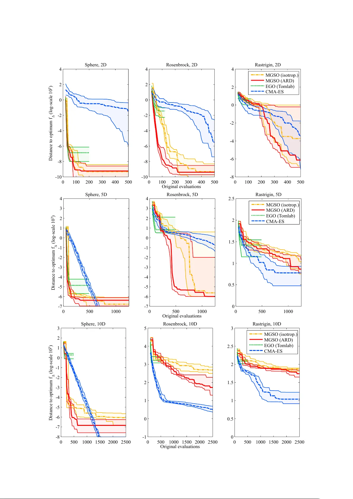
Model Guided Sampling Optimization for Lo w-dimensional Problems Lukáš Bajer 1,2 and Martin Hole ˇ na 1 1 Institute of Computer Science, Academy of Sciences of the Czech Republic, Pod V odárenskou v ˇ eží 2, Prague 2 Faculty of Mathematics and Physics, Charles Uni v ersity in Prague, Malostranské nám. 25, Prague Nov ember 20, 2021 ArXiv .org preprint original article published by SCITEPRESS – Science and T echnology Publications in ICAART 2015 Pr oceedings of the International Confer ence on Agents and Artificial Intelligence, V olume 2 ISBN 978-989-758-074-1 Abstract Optimization of v ery expensi ve black-box functions requires utilization of maximum information g ath- ered by the process of optimization. Model Guided Sampling Optimization (MGSO) forms a more robust alternativ e to Jones’ Gaussian-process-based EGO algorithm. Instead of EGO’ s maximizing expected im- prov ement, the MGSO uses sampling the probability of improvement which is sho wn to be helpful against trapping in local minima. Further , the MGSO can reach close-to-optimum solutions faster than standard optimization algorithms on low dimensional or smooth problems. Keyw ords : black-box optimization, Gaussian process, surrogate modelling, EGO 1 1 INTR ODUCTION Optimization of expensi ve empirical functions forms an important topic in many engineering or natural- sciences areas. For such functions, it is often impossible to obtain any derivati ves or information about smoothness; moreover , there is no mathematical expression nor an algorithm to ev aluate. Instead, some simulation or experiment has to be performed, and the v alue obtained through a simulation or e xperiment is the value of the objecti ve function being considered. Such functions are also called black-box functions. They are usually v ery expensiv e to ev aluate; one ev aluation may cost a lot of time and money to process. Because of the absence of derivati ves, standard continuous first- or second-order deriv ativ e optimiza- tion methods cannot be used. In addition, the functions of this kind are usually characterized by a high number of local optima where simple algorithms can be trapped easily . Therefore, different deri vati ve-free optimization methods (often called meta-heuristics) hav e been proposed. Even though these methods are rather slow and sometimes also computationally intensive, the cost of the empirical function ev aluations is always much higher and the cost of these e valuations dominates the computational cost of the optimization algorithm. F or this reason, it is crucial to decrease the number of function e valuations as much as possible. Evolutionary algorithms constitute a broad f amily of meta-heuristics that are frequently used for black- box optimization. Furthermore, some additional algorithms and techniques ha ve been designed to minimize the number of objectiv e function ev aluations. All of the three follo wing approaches use a model (of a different type in each case), which is b uilt and updated within the optimization process. Estimation of distribution algorithms (ED As) [Larrañaga and Lozano, 2002] represent one such ap- proach: EDAs iterati vely estimate the distribution of selected solutions (usually solutions with fitness abov e some threshold) and sample this distribution forming a ne w set of solutions for the next iteration. Surr ogate modelling is the technique of learning and usage of a re gression model of the objecti ve func- tion [Jin, 2005]. The model (called surrogate model in this context) is then used to ev aluate some of the candidate solutions instead of the original costly objectiv e function. Our method, Model Guided Sampling Optimization (MGSO), takes inspiration from both these ap- proaches. It uses a re gression model of the objectiv e function, which also provides an error estimate. Howe ver , instead of replacing the objectiv e function with this model, it combines its prediction and the error estimate to get a probability of reaching a better solution in a giv en point. Similarly to EDAs, the MGSO then samples this pseudo-distribution 1 , in order to obtain the next set of solution candidates. The MGSO is also similar to Jones’ Efficient Global Optimization (EGO) [Jones et al., 1998]. Like EGO, the MGSO uses a Gaussian process (GP , see [Rasmussen and Williams, 2006] for reference), which provides a guide where to sample new candidate solutions in order to explore new areas and e xploit promis- ing parts of the objecti ve-function landscape. Where EGO selects a single or very fe w solutions maximizing a chosen criterion – Expected Improv ement (EI) or Probability of Improvement (PoI) – the MGSO samples the latter criterion. At the same time, the GP serv es for the MGSO as a surrogate model of the objective function for a small proportion of the solutions. This paper further develops the MGSO algorithm introduced in [Bajer et al., 2013]. It brings sev eral improv ements (new optimization procedures and more general co variance function) and performance com- parison to EGO. The following section introduces methods used in the MGSO, Section 3 describes the MGSO algorithm, and Section 4 comprises some e xperimental results on several functions from the BBOB testing set [Hansen et al., 2009]. 2 GA USSIAN PROCESSES Gaussian process is a probabilistic model based on Gaussian distributions. This type of model was chosen because it predicts the function value in a ne w point in the form of univariate Gaussian distribution: the mean and the standard deviation of the function value are provided. Through the predicted mean, the GP can serve as a surrogate model, and the standard deviation is an estimate of the prediction uncertainty in a new point. 1 a function proportional to a probability distribution, it’ s v alue is giv en by the probability of impr ovement 2 The GP is specified by mean and cov ariance functions and a relatively small number of covariance function’ s hyper -parameters. The hyper-parameters are usually fitted by the maximum-lik elihood method. Let X N = { x i | x i ∈ R D } N i = 1 be a set of N training D -dimensional data points with known dependent- variable values y N = { y i } N i = 1 and f ( x ) be an unknown function being modelled for which f ( x i ) = y i for all i ∈ { 1 , . . . , N } . The GP model imposes a probabilistic model on the data: the vector of known function values y N is considered to be a sample of a N -dimensional multiv ariate Gaussian distribution with the value of the probability density p ( y N | X N ) . If we take into consideration a new data point ( x N + 1 , y N + 1 ) , the v alue of the probability density in the new point is p ( y N + 1 | X N + 1 ) = exp ( − 1 2 y > N + 1 C − 1 N + 1 y N + 1 ) p ( 2 π ) N + 1 det ( C N + 1 ) (1) where C N + 1 is the cov ariance matrix of the Gaussian distribution (for which mean is usually set to constant zero) and y N + 1 = ( y 1 , . . . , y N , y N + 1 ) (see [Buche et al., 2005] for details). This cov ariance can be written as C N + 1 =  C N k k > κ  (2) where C N is the covariance of the Gaussian distribution gi ven the N training data points, k is the vector of cov ariances between the new point and training data, and κ is the variance of the ne w point itself. Predictions. Predictions in Gaussian processes are made using Bayesian inference. Since the in verse C − 1 N + 1 of the extended cov ariance matrix can be expressed using the in verse of the training co variance C − 1 N , and y N is known, the density of the distribution in a new point simplifies to a univ ariate Gaussian with the density p ( y N + 1 | X N + 1 , y N ) ∝ exp − 1 2 ( y N + 1 − ˆ y N + 1 ) 2 s 2 y N + 1 ! (3) with the mean and variance gi ven by ˆ y N + 1 = k > C − 1 N y N , (4) s 2 y N + 1 = κ − k > C − 1 N k . (5) Further details can be found in [Buche et al., 2005]. Covariance functions. The cov ariance C N plays a crucial role in these equations. It is defined by the cov ariance-function matrix K and signal noise σ as C N = K N + σ I N (6) where I N is the identity matrix of order N . Gaussian processes use parametrized cov ariance functions K describing prior assumptions on the shape of the modelled function. The cov ariance between the function values at tw o data points x i and x j is gi ven by K ( x i , x j ) , which forms the ( i , j ) -th element of the matrix K N . W e used the most common squared-exponential function K ( x i , x j ) = θ exp  − 1 2 ` 2 ( x i − x j ) > ( x i − x j )  , (7) which is suitable when the modelled function is rather smooth. The closer the points x i and x j are, the closer the cov ariance function value is to 1 and the stronger correlation between the function values f ( x i ) and f ( x j ) is. The signal variance θ scales this correlation, and the parameter ` is the characteristic length- scale with which the distance of two considered data points is compared. Our choice of the covariance function was moti vated by its simplicity and the possibility of finding the hyper-parameter values by the maximum-likelihood method. 3 −5 0 5 −5 0 5 0.1 0.2 0.3 0.4 0.5 0.6 0.7 0.8 0.9 Figure 1: Probability of improv ement. Rastrigin function in 2D, the GP model is built using 40 data points. 3 MODEL GUIDED SAMPLING OPTIMIZA TION (MGSO) The MGSO algorithm is based on a similar idea as EGO. It heavily relies on Gaussian process modelling, particularly on its regression capabilities and ability to assess model uncertainty in any point of the input space. While most variants of EGO calculate new points from the expected impro vement (EI), The MGSO utilizes the probability of impr ovement which is closer to the basic concept of the MGSO: sampling a distribution of promising solutions 2 . This probability is taken as a function proportional to a probability density and is sampled producing a whole population of candidate solutions – indi viduals. This is the main dif ference to EGO which takes only very fe w individuals each iteration, usually the point maximizing EI. 3.1 Sampling The core step of the MGSO algorithm is the sampling of the probability of improvement. This probability is, for a chosen threshold T of the function value, directly giv en by the predicted mean ˆ f ( x ) = ˆ y and the standard deviation ˆ s ( x ) = s y of the GP model ˆ f in any point x of the input space PoI T ( x ) = P ( ˆ f ( x ) 5 T ) = Φ  T − ˆ f ( x ) ˆ s ( x )  , (8) which corresponds to the value of cumulativ e distribution function (CDF) of the Gaussian with density (3) for the value of threshold T . As a threshold T , v alues near the so-far optimum (or the global optimum if known) are usually tak en. Even though all the variables come from Gaussian distribution, PoI ( x ) is definitely not Gaussian-shaped since it depends on the threshold T and the black-box function being modelled f . A typical example of the landscape of PoI ( x ) in two dimensions for the Rastrigin function is depicted in Fig. 1. The dependency on the black-box function also causes the lack of analytical marginals or deri vati ves. 3.2 MGSO Procedur e The MGSO algorithm starts with an initial random sample from the input space forming an initial pop- ulation, which is evaluated with the black-box objectiv e function (step (2) in Alg. 1). All the evaluated solutions are sav ed to a database from where they are used as a training set for the GP model. The main c ycle of the MGSO starts with fitting the GP model’ s ( M i ) hyper-parameters based on the data from the current dataset S i (step (4)). Further, the model’ s PoI M i T is sampled (step (5)) and supplemented with the GP model’ s minimum (step (6)), forming up to N new individuals { x j } N j = 1 where N is a parameter defining the standard population size. The algorithm follows up with the evaluation of the new indi viduals 2 some EGO variants use PoI, too [Jones, 2001] 4 Algorithm 1 MGSO (Model Guided Sampling Optimization) 1: Input : f – black-box objective function N – standard population size r – the number of solutions for dataset restriction 2: S 0 = { ( x j , y j ) } N j = 1 ← generate N initial samples and ev aluate them by f : y j = f ( x j ) 3: while no stopping condition is met, for i = 1 , 2 , . . . do 4: M i ← build a GP model and fit its hyper -parameters according to the dataset S i − 1 5: { x j } N j = 1 ← sample the PoI M i T ( x ) forming N new points, optionally with dif ferent targets T 6: x min ← arg min x ˆ f ( x ) – find the minimum of the GP (by local cont. optimization) and replace the nearest solution from { x j } N j = 1 with it 7: { y j } N j = 1 ← f ( { x j } N j = 1 ) {ev aluate the population} 8: S i ← S i − 1 ∪ { ( x j , y j ) } N j = 1 {augment the dataset} 9: ( x min , y min ) ← arg min ( x , y ) ∈ S i y {find the best solution in S i } 10: if any rescale condition is met then 11: restrict the dataset S i to the bounding-box [ l i , u i ] of the r nearest solutions along the best solution ( x min , y min ) and linearly transform S i to [ − 1 , 1 ] D 12: end if 13: end while 14: Output : the best found solution ( x min , y min ) with the objectiv e function (step (7)), extending the dataset of already-measured samples (step (8)) and finding the best so-far optimum ( x min , y min ) (step (9)). Covariance matrix constraint. As every cov ariance matrix, Gaussian process’ cov ariance matrix is required to be positive semi-definite (PSD). This constraint is checked during sampling, and candidate solutions leading to close-to-indefinite matrix are rejected. Although it could cause smaller population- size in some iterations, it is an important step: otherwise, Gaussian process training and fitting becomes numerically v ery unstable. If such rejections arise, other two thresholds T for calculating PoI are tested and population with the greatest cardinality is taken. These rejections occur when the GP model is sufficiently trained and sampled solutions become close to the model’ s predicted v alues. Model minimum. New population is supplemented with the minimum x min of the model’ s predicted values found by continuous optimization 3 (step (6), x min = arg min x ˆ f ( x ) ); more precisely , the nearest sampled solution is replaced with this minimum (unless less than N solutions were sampled). Input space restriction. In current implementation, MGSO requires bounds constraints x ∈ [ l , u ] , l < u ∈ R D to be defined on the input space, which is used by the algorithm to internal linear scaling of the input space to hypercube [ − 1 , 1 ] D . As the algorithm proceeds, the input space can be restricted along the so-far optimum to a smaller bounding box (steps (10)–(12)) which is again linearly scaled to [ − 1 , 1 ] D . The size of the new box is defined as a bounding box of r nearest samples from the current so-far optimum x min ; enlarged by 10% at the boundaries. For the parameter r = 15 · D was used as a rule of thumb. This process not only speeds up model fitting and prediction (due to the smaller number of training data), but focuses the optimization along the best found solution and broaden small regions of non-zero PoI. Sev eral criteria are defined to launch such input space restriction, from which the most important is occurrence of numerous rejections in sampling due to close-to-indefinite cov ariance matrix. If the resulting 3 Matlab’ s fminsearch was used 5 new bounding box from the restriction is close to the previous box (the coordinates are not smaller than [ − 0 . 8 , 0 . 8 ] D ), the input space restriction is not performed. 3.3 Gaussian Processes Implementation Our Matlab implementation of the MGSO makes use of Gaussian Process Regression and Classification T oolbox (GPML Matlab code) – a toolbox accompanying Rasmussen’ s and W illiams’ monograph [Rasmussen and Williams, 2006]. In the current v ersion of the MGSO, Rasmussen’ s optimization and model fitting procedure minimize was replaced with fmincon from Matlab Optimization toolbox and with Hansen’ s Covariance Matrix Adap- tation (CMA-ES) [Hansen and Ostermeier , 2001]. These functions are used for the minimization of GP’ s negati ve log-likelihood in model’ s hyper-parameters fitting. Here, fmincon is generally faster , but CMA-ES is more robust and does not need a v alid initial point. The next improvement lies in the employment of the diagonal-matrix characteristic length-scale pa- rameter in the squared exponential covariance function, sometimes also called covariance function with automatic relev ance determination (ARD) K ARD ( x i , x j ) = θ exp  − 1 2 ( x i − x j ) > diag ( ~ ` ) ( x i − x j )  . (9) The length-scale parameter ` in (7) changes to diag ( ~ ` ) – a matrix with diagonal elements formed by the elements of the vector ~ ` ∈ R D . The application of ARD was not straightforw ard, because hyper -parameters training tends to stuck in local optima. These cases were indicated by an extreme difference between the different scale-length parameter ~ ` components which resulted in poor regression capabilities. Therefore, constraints on maximum difference between components of ~ ` were introduced ~ ` i ≤ 2 . 5 k median ( ~ ` ) − ~ ` i k . 4 EXPERIMENT AL RESUL TS This section comprises quantitativ e results from several tests of the MGSO as well as brief discussion of the usability of the algorithm. The current Matlab implementation of the MGSO algorithm 4 has been tested on three different benchmark functions from the BBOB testing set [Hansen et al., 2009]: sphere, Rosenbrock and Rastrigin function in three different dimensionalities: 2D, 5D and 10D. For these cases, comparison with CMA-ES – current state of the art black-box optimization algorithm – and T omlab’ s implementation of EGO 5 is provided. The computational times are not quantified, but whereas CMA-ES performs in orders of tens of sec- onds, the running times of the MGSO and EGO reaches up to several hours. W e consider this drawback acceptable since the primary use of the MGSO is expensiv e black box optimization where a single ev alua- tion of the objectiv e function can easily take man y hours or e ven days and/or cost a considerable amount of money [Hole ˇ na et al., 2008]. In the case of two-dimensional problems , the MGSO performs far better than CMA-ES on quadratic sphere and Rosenbrock function. The results on Rastrigin function are comparable, although with greater variance (see Fig. 2: the descent of the medians is slightly slower within the first 200 function ev aluations, but faster thereafter). The T omlab’ s implementation of EGO performs almost equally well as the MGSO on sphere function, b ut on Rosenbrock and Rastrigin, the con vergence of EGO is extremely slowed down after fe w iterations, which can be seen in 5D and 10D, too. The positiv e effect of ARD cov ariance function can be seen quite clearly , especially on Rosenbrock function. The difference between ARD and non-ARD 4 the source is av ailable at http://github.com/charypar/gpeda 5 http://tomopt.com/tomlab/products/cgo/solvers/ego.php 6 Sphere, 2D Distance to optimum f Δ (log-scale 10 y ) 0 100 200 300 400 500 -10 -8 -6 -4 -2 0 2 4 Rosenbrock, 2D Original evaluations 0 100 200 300 400 500 -10 -8 -6 -4 -2 0 2 4 Rastrigin, 2D 0 100 200 300 400 500 -8 -6 -4 -2 0 2 4 MGSO (isotrop.) MGSO (ARD) EGO (T omlab) CMA-ES Sphere, 5D Distance to optimum f Δ (log-scale 10 y ) 0 500 1000 -7 -6 -5 -4 -3 -2 -1 0 1 2 3 4 Rosenbrock, 5D Original evaluations 0 500 1000 -7 -6 -5 -4 -3 -2 -1 0 1 2 3 4 Rastrigin, 5D 0 500 1000 0 0.5 1 1.5 2 2.5 MGSO (isotrop.) MGSO (ARD) EGO (T omlab) CMA-ES Sphere, 10D Distance to optimum f Δ (log-scale 10 y ) 0 500 1000 1500 2000 2500 -8 -7 -6 -5 -4 -3 -2 -1 0 1 2 3 Rosenbrock, 10D Original evaluations 0 500 1000 1500 2000 2500 -1 0 1 2 3 4 5 Rastrigin, 10D 0 500 1000 1500 2000 2500 0 0.5 1 1.5 2 2.5 3 MGSO (isotrop.) MGSO (ARD) EGO (T omlab) CMA-ES Figure 2: Medians, and the first and third quartiles of the distances from the best individual to optimum ( f ∆ = f best − f OPT ) with respect to the number of objective function ev aluations for three benchmark functions. Quartiles are computed out of 15 trials with different initial settings (instances 1–5 and 31–40 in the BBOB frame work). 7 results are hardly to see on sphere function, probably because its symmetry means no impro vement in ARD cov ariance employment. The performance of the MGSO on five-dimensional problems is similar to 2D cases. The MGSO de- scends notably faster on non-rugged sphere and Rosenbrock functions, especially if we concentrate on depicted cases with a very lo w number of objectiv e function ev aluations (up to 250 · D ev aluations). The drawbacks of the MGSO is shown on 5D Rastrigin function where it is outperformed by CMA-ES, espe- cially between ca. 200 and 1200 function e valuations. Results of optimization in the case of ten-dimensional pr oblems show that the MGSO works better than CMA-ES only on the most smooth sphere function which is very easy to regress by Gaussian process model. On more complicated benchmarks, the MGSO is outperformed by CMA-ES. The graphs on Fig. 2 show that the MGSO is usually slightly slower than EGO in the very first phases of the optimization, b ut EGO quickly stops its progress and does not descent further . This is exactly what can be expected from the MGSO in comparison to EGO – sampling the PoI instead of searching for the maximum can easily ov ercome situations where EGO gets stuck in a local optimum. 5 CONCLUSIONS AND FUTURE WORK The MGSO, the optimization algorithm based on a Gaussian process model and the sampling of the prob- ability of improvement, is intended to be used in the field of expensi ve black-box optimization. This paper summarizes its properties and ev aluates its performance on sev eral benchmark problems. Comparison with Gaussian-process based EGO algorithm sho ws that the MGSO is able to easily escape from local optima. Further , it has been shown that the MGSO can outperform state-of-the-art continuous black-box optimiza- tion algorithm CMA-ES in lo w dimensionalities or on very smooth functions. On the other hand, CMA-ES performs better on rugged or high-dimensional benchmarks. A CKNO WLEDGEMENTS This work was supported by the Czech Science F oundation (GA ˇ CR) grants P202/10/1333 and 13-17187S. Refer ences [Bajer et al., 2013] Bajer , L., Hole ˇ na, M., and Charypar , V . (2013). Improving the model guided sampling optimization by model search and slice sampling. In V inar , T . e. a., editor , IT A T 2013 – W orkshops, P osters, and T utorials , pages 86–91. CreateSpace Indp. Publ. Platform. [Buche et al., 2005] Buche, D., Schraudolph, N., and Koumoutsakos, P . (2005). Accelerating e volutionary algorithms with gaussian process fitness function models. IEEE T ransactions on Systems, Man, and Cybernetics, P art C: Applications and Reviews , 35(2):183–194. [Hansen et al., 2009] Hansen, N., Finck, S., Ros, R., and Auger, A. (2009). Real-parameter black-box optimization benchmarking 2009: Noiseless functions definitions. T echnical Report RR-6829, INRIA. Updated February 2010. [Hansen and Ostermeier , 2001] Hansen, N. and Ostermeier , A. (2001). Completely derandomized self- adaptation in ev olution strategies. Evolutionary Computation , 9(2):159–195. [Hole ˇ na et al., 2008] Hole ˇ na, M., Cukic, T ., Rodemerck, U., and Linke, D. (2008). Optimization of cata- lysts using specific, description based genetic algorithms. Journal of Chemical Information and Model- ing , 48:274–282. [Jin, 2005] Jin, Y . (2005). A comprehensi ve survey of fitness approximation in ev olutionary computation. Soft Computing , 9(1):3–12. 8 [Jones, 2001] Jones, D. R. (2001). A taxonomy of global optimization methods based on response surfaces. Journal of Global Optimization , 21(4):345–383. [Jones et al., 1998] Jones, D. R., Schonlau, M., and W elch, W . J. (1998). Efficient global optimization of expensi ve black-box functions. Journal of Global Optimization , 13(4):455–492. [Larrañaga and Lozano, 2002] Larrañaga, P . and Lozano, J. A. (2002). Estimation of distribution algo- rithms: A new tool for e volutionary computation . Kluwer . [Rasmussen and W illiams, 2006] Rasmussen, C. E. and W illiams, C. K. I. (2006). Gaussian Pr ocesses for Machine Learning . Adaptative computation and machine learning series. MIT Press. 9