Fast and Flexible ADMM Algorithms for Trend Filtering

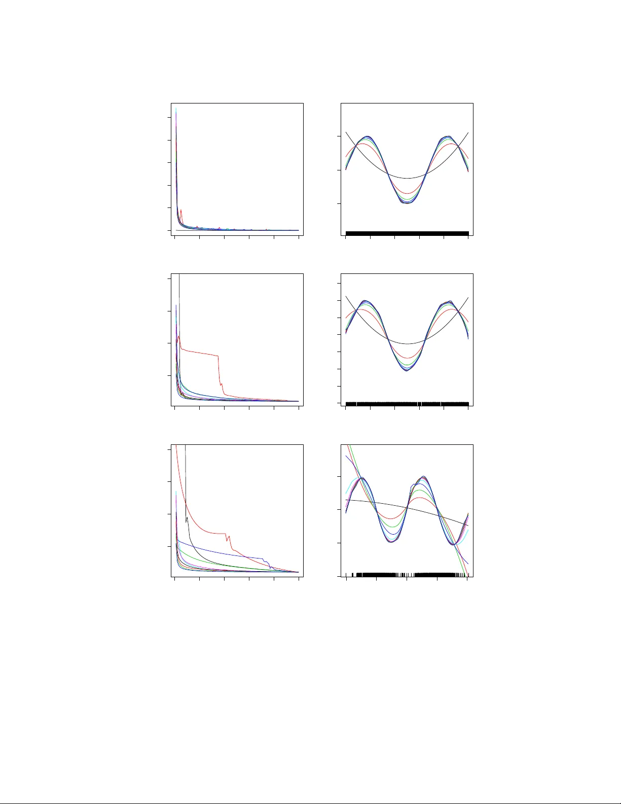
F ast and Flexible ADMM Algorithms for T rend Filtering Aadit y a Ramdas 21 aramdas@cs.cmu.edu Ry an J. Tibshirani 12 ryantibs@stat.cmu.edu 1 Departmen t of Statistics and 2 Mac hine Learning Departmen t Carnegie Mellon Univ ersit y Abstract This pap er presents a fast and robust algorithm for trend filtering, a recen tly dev eloped nonparametric regression to ol. It has b een sho wn that, for estimating functions whose deriv a- tiv es are of b ounded v ariation, trend filtering achiev es the minimax optimal error rate, while other p opular metho ds like smo othing splines and k ernels do not. Standing in the wa y of a more widespread practical adoption, how ev er, is a lack of scalable and numerically stable al- gorithms for fitting trend filtering estimates. This pap er presen ts a highly efficient, sp ecialized ADMM routine for trend filtering. Our algorithm is comp etitiv e with the specialized interior p oin t metho ds that are currently in use, and yet is far more numerically robust. F urthermore, the prop osed ADMM implementation is very simple, and importantly , it is flexible enough to extend to many in teresting related problems, suc h as sparse trend filtering and isotonic trend filtering. Softw are for our metho d is freely av ailable, in b oth the C and R languages. 1 In tro duction T rend filtering is a relatively new method for nonparametric regression, prop osed indep enden tly by Steidl et al. (2006), Kim et al. (2009). Supp ose that we are giv en output points y = ( y 1 , . . . y n ) ∈ R n , observ ed across ev enly spaced input points x = ( x 1 , . . . x n ) ∈ R n , sa y , x 1 = 1 , . . . x n = n for simplicit y . The trend filtering estimate ˆ β = ( ˆ β 1 , . . . ˆ β n ) ∈ R n of a sp ecified order k ≥ 0 is defined as ˆ β = argmin β ∈ R n 1 2 k y − β k 2 2 + λ k D ( k +1) β k 1 . (1) Here λ ≥ 0 is a tuning parameter, and D ( k +1) ∈ R ( n − k ) × n is the discrete difference (or deriv ativ e) op erator of order k + 1. W e can define these op erators recursively as D (1) =      − 1 1 0 . . . 0 0 0 − 1 1 . . . 0 0 . . . 0 0 0 . . . − 1 1      , (2) and D ( k +1) = D (1) D ( k ) for k = 1 , 2 , 3 , . . . . (3) (Note that, ab o ve, we write D (1) to mean the ( n − k − 1) × ( n − k ) version of the 1st order difference matrix in (2).) When k = 0, w e can see from the definition of D (1) in (2) that the trend filtering problem (1) is the same as the 1-dimensional fused lasso problem (Tibshirani et al. 2005), also called 1-dimensional total v ariation denoising (Rudin et al. 1992), and hence the 0th order trend filtering estimate ˆ β is piecewise constant across the input p oints x 1 , . . . x n . 1 F or a general k , the k th order trend filtering estimate has the structure of a k th order piecewise p olynomial function, ev aluated across the inputs x 1 , . . . x n . The knots in this piecewise p olynomial are selected adaptiv ely among x 1 , . . . x n , with a higher v alue of the tuning parameter λ (generally) corresp onding to fewer knots. T o see examples, the reader can jump ahead to the next subsection, or to future sections. F or arbitrary input points x 1 , . . . x n (i.e., these need not b e ev enly spaced), the defined difference op erators will hav e different nonzero en tries, but their structure and the recursive relationship b et w een them is basically the same; see Section 4. Broadly sp eaking, nonparametric regression is a well-studied field with many celebrated tools, and so one may wonder about the merits of trend filtering in particular. F or detailed motiv ation, w e refer the reader to Tibshirani (2014), where it is argued that trend filtering essentially balances the strengths of smo othing splines (de Bo or 1978, W ahba 1990) and lo cally adaptiv e regression splines (Mammen & v an de Geer 1997), which are tw o of the most common tools for piecewise p olynomial estimation. In short: smo othing splines are highly computationally efficien t but are not minimax optimal (for estimating functions whose deriv ativ es are of bounded v ariation); lo cally adaptiv e regression splines are minimax optimal but are relativ ely inefficien t in terms of computation; trend filtering is b oth minimax optimal and computationally comparable to smo othing splines. Tibshirani (2014) fo cuses mainly on the statistical prop erties trend filtering estimates, and relies on externally deriv ed algorithms for comparisons of computational efficiency . 1.1 Ov erview of con tributions In this pap er, w e prop ose a new algorithm for trend filtering. W e do not explicitly address the problem of mo del selection, i.e., we do not discuss ho w to c hoose the tuning parameter λ in (1), whic h is a long-standing statistical issue with an y regularized estimation metho d. Our concern is computational; if a practitioner wan ts to solve the trend filtering problem (1) at a giv en v alue of λ (or sequence of v alues), then we provide a scalable and efficien t means of doing so. Of course, a fast algorithm such as the one we pro vide can still b e helpful for model selection, in that it can provide sp eedups for common techniques like cross-v alidation. F or 0th order trend filtering, i.e., the 1d fused lasso problem, tw o direct, linear time algorithms already exist: the first uses a taut string principle (Davies & Kov ac 2001), and the second uses an en tirely differen t dynamic programming approac h (Johnson 2013). Both are extremely (and equally) fast in practice, and for this sp ecial 0th order problem, these tw o direct algorithms rise ab o v e all else in terms of computational efficiency and numerical accuracy . As far as we know (and despite our b est attempts), these algorithms cannot be directly extended to the higher order cases k = 1 , 2 , 3 , . . . . Ho wev er, our proposal indir e ctly extends these formidable algorithms to the higher order cases with a sp ecial implementation of the alternating direction method of m ultipliers (ADMM). In general, there can b e multiple w a ys to reparametrize an unconstrained optimization problem so that ADMM can b e applied; for the trend filtering problem (1), we c ho ose a particular parametrization suggested b y the recursive decomp osition (3), lev eraging the fast, exact algorithms that exist for the k = 0 case. W e find that this choice makes a big difference in terms of the conv ergence of the resulting ADMM routine, compared to what may be considered the standard ADMM parametrization for (1). Curren tly , the sp ecialized primal-dual interior p oint (PDIP) metho d of Kim et al. (2009) seems to b e the preferred metho d for computing trend filtering estimates. The iterations of this algorithm are c heap because they reduce to solving banded linear systems (the discrete difference operators are themselv es banded). Our sp ecialized ADMM implementation and the PDIP metho d ha v e distinct strengths. W e summarize our main findings b elo w. • Our sp ecialized ADMM implementation conv erges more reliably than the PDIP metho d, ov er a wide range of problems sizes n and tuning parameter v alues λ . • In particular setups—namely , small problem sizes, and small v alues of λ for moderate and large problem sizes—the PDIP metho d conv erges to high accuracy solutions very rapidly . In 2 suc h situations, our sp ecialized ADMM algorithm do es not match the conv ergence rate of this second-order metho d. • How ev er, when plotting the function estimates, our sp ecialized ADMM implementation pro- duces solutions of visually p erfectly acceptable accuracy after a small num ber of iterations. This is true ov er a broad range of problem sizes n and parameter v alues λ , and cov ers the set- tings in which its achiev ed criterion v alue has not con verged at the rate of the PDIP metho d. • F urthermore, our sp ecialized ADMM implementation displa ys a greatly improv ed con vergence rate ov er what may b e thought of as the “standard” ADMM implementation for problem (1). Lo osely sp eaking, standard implemen tations of ADMM are generally considered to b eha v e lik e first-order metho ds (Boyd et al. 2011), whereas our sp ecialized implemen tation exhibits p erformance somewhere in b et w een that of a first- and second-order metho d. • One iteration of our sp ecialized ADMM implementation has linear complexity in the problem size n ; this is also true for PDIP . Empirically , an iteration of our ADMM routine runs ab out 10 times faster than a PDIP iteration. • Our specialized ADMM implementation is quite simple (considerably simpler than the sp e- cialized primal-dual interior p oin t metho d), and is flexible enough that it can b e extended to co ver many v arian ts and extensions of the basic trend filtering problem (1), such as sparse trend filtering, mixed trend filtering, and isotonic trend filtering. • Finally , it is w orth remarking that extensions beyond the univ ariate case are readily a v ailable as w ell, as univ ariate nonparametric regression tools can b e used as building blocks for estimation in broader mo del classes, e.g., in generalized additive mo dels (Hastie & Tibshirani 1990). Readers well-v ersed in optimization may wonder ab out alternativ e iterative (descent) metho ds for solving the trend filtering problem (1). Two natural candidates that ha v e enjo yed muc h success in lasso regression problems are proximal gradien t and co ordinate descen t algorithms. Next, we giv e a motiv ating case study that illustrates the inferior p erformance of both of these metho ds for trend filtering. In short, their p erformance is hea vily affected b y p o or conditioning of the difference op erator D ( k +1) , and their conv ergence is many orders of magnitude w orse than the specialized primal-dual in terior p oin t and ADMM approaches. 1.2 A motiv ating example Conditioning is a subtle but ever-presen t issue faced by iterative (indirect) optimization metho ds. This issue affects some algorithms more than others; e.g., in a classical optimization con text, it is w ell-understoo d that the conv ergence bounds for gradien t descen t depend on the smallest and largest eigenv alues of the Hessian of the criterion function, while those for Newton’s method do not (Newton’s metho d b eing affine in v arian t). Unfortunately , conditioning is a very real issue when solving the trend filtering problem in (1)—the discrete deriv ativ e op erators D ( k +1) , k = 0 , 1 , 2 , . . . are extremely ill-conditioned, and this only w orsens as k increases. This worry can be easily realized in examples, as w e no w demonstrate in a simple simulation with a reasonable p olynomial order, k = 1, and a mo dest problem size, n = 1000. F or solving the trend filtering problem (1), with λ = 1000, we compare proximal gradient descent and accelerated pro ximal gradient metho d (performed on b oth the primal and the dual problems), coordinate descen t, a standard ADMM approach, our specialized ADMM approach, and the sp ecialized PDIP metho d of Kim et al. (2009). Details of the sim ulation setup and these v arious algorithms are giv en in App endix A.1, but the main message can b e seen from Figure 1. Differen t v arian ts of pro ximal gradien t metho ds, as well as coordinate descent, and a standard ADMM approach, all p erform quite p oorly in computing trend filtering estimate, but the second-order PDIP method and our spe cialized 3 ADMM implemen tation p erform drastically better—these t wo reac h in 20 iterations what the others could not reach in many thousands. Although the latter tw o techniques p erform similarly in this example, we will see later that our sp ecialized ADMM approach generally suffers from far less conditioning and con vergence issues than PDIP , esp ecially in regimes of regularization (i.e., ranges of λ v alues) that are most in teresting statistically . The rest of this pap er is organized as follows. In Section 2, we describ e our sp ecialized ADMM implemen tation for trend filtering. In Section 3, we mak e extensive comparisons to PDIP . Section 4 co v ers the case of general input p oin ts x 1 , . . . x n . Section 5 considers sev eral extensions of the basic trend filtering mo del, and the accompanying adaptions of our specialized ADMM algorithm. Section 6 concludes with a short discussion. 2 A sp ecialized ADMM algorithm W e describ e a sp ecialized ADMM algorithm for trend filtering. This algorithm may app ear to only sligh tly differ in its construction from a more standard ADMM algorithm for trend filtering, and b oth approaches hav e virtually the same computational complexit y , requiring O ( n ) op erations p er iteration; how ev er, as we ha ve glimpsed in Figure 1, the difference in conv ergence b et w een the tw o is drastic. The standard ADMM approac h (e.g., Boyd et al. (2011)) is based on rewriting problem (1) as min β ∈ R n , α ∈ R n − k − 1 1 2 k y − β k 2 2 + λ k α k 1 sub ject to α = D ( k +1) β . (4) The augmen ted Lagrangian can then b e written as L ( β , α, u ) = 1 2 k y − β k 2 2 + λ k α k 1 + ρ 2 k α − D ( k +1) β + u k 2 2 − ρ 2 k u k 2 2 , from whic h we can derive the standard ADMM up dates: β ←  I + ρ ( D ( k +1) ) T D ( k +1)  − 1  y + ρ ( D ( k +1) ) T ( α + u )  , (5) α ← S λ/ρ ( D ( k +1) β − u ) , (6) u ← u + α − D ( k +1) β . (7) The β -up date is a banded linear system solve, with bandwidth k + 2, and can b e implemented in time O ( n ( k + 2) 2 ) (actually , O ( n ( k + 2) 2 ) for the first solv e, with a banded Cholesky , and O ( n ( k + 2)) for each subsequent solve). The α -up date, where S λ/ρ denotes co ordinate-wise soft-thresholding at the level λ/ρ , takes time O ( n − k − 1). The dual up date uses a banded matrix multiplication, taking time O ( n ( k + 2)), and therefore one full iteration of standard ADMM up dates can b e done in linear time (considering k as a constan t). Our sp ecialized ADMM approach instead b egins b y rewriting (1) as min β ∈ R n , α ∈ R n − k 1 2 k y − β k 2 2 + λ k D (1) α k 1 sub ject to α = D ( k ) β , (8) where w e hav e used the recursive prop ert y D ( k +1) = D (1) D ( k ) . The augmented Lagrangian is now L ( β , α, u ) = 1 2 k y − β k 2 2 + λ k D (1) α k 1 + ρ 2 k α − D ( k ) β + u k 2 2 − ρ 2 k u k 2 2 , yielding the sp ecialized ADMM up dates: β ←  I + ρ ( D ( k ) ) T D ( k )  − 1  y + ρ ( D ( k ) ) T ( α + u )  , (9) α ← argmin α ∈ R n − k 1 2 k D ( k ) β − u − α k 2 2 + λ/ρ k D (1) α k 1 , (10) u ← u + α − D ( k ) β . (11) 4 ● ● ● ● ● ● ● ● ● ● ● ● ● ● ● ● ● ● ● ● ● ● ● ● ● ● ● ● ● ● ● ● ● ● ● ● ● ● ● ● ● ● ● ● ● ● ● ● ● ● ● ● ● ● ● ● ● ● ● ● ● ● ● ● ● ● ● ● ● ● ● ● ● ● ● ● ● ● ● ● ● ● ● ● ● ● ● ● ● ● ● ● ● ● ● ● ● ● ● ● ● ● ● ● ● ● ● ● ● ● ● ● ● ● ● ● ● ● ● ● ● ● ● ● ● ● ● ● ● ● ● ● ● ● ● ● ● ● ● ● ● ● ● ● ● ● ● ● ● ● ● ● ● ● ● ● ● ● ● ● ● ● ● ● ● ● ● ● ● ● ● ● ● ● ● ● ● ● ● ● ● ● ● ● ● ● ● ● ● ● ● ● ● ● ● ● ● ● ● ● ● ● ● ● ● ● ● ● ● ● ● ● ● ● ● ● ● ● ● ● ● ● ● ● ● ● ● ● ● ● ● ● ● ● ● ● ● ● ● ● ● ● ● ● ● ● ● ● ● ● ● ● ● ● ● ● ● ● ● ● ● ● ● ● ● ● ● ● ● ● ● ● ● ● ● ● ● ● ● ● ● ● ● ● ● ● ● ● ● ● ● ● ● ● ● ● ● ● ● ● ● ● ● ● ● ● ● ● ● ● ● ● ● ● ● ● ● ● ● ● ● ● ● ● ● ● ● ● ● ● ● ● ● ● ● ● ● ● ● ● ● ● ● ● ● ● ● ● ● ● ● ● ● ● ● ● ● ● ● ● ● ● ● ● ● ● ● ● ● ● ● ● ● ● ● ● ● ● ● ● ● ● ● ● ● ● ● ● ● ● ● ● ● ● ● ● ● ● ● ● ● ● ● ● ● ● ● ● ● ● ● ● ● ● ● ● ● ● ● ● ● ● ● ● ● ● ● ● ● ● ● ● ● ● ● ● ● ● ● ● ● ● ● ● ● ● ● ● ● ● ● ● ● ● ● ● ● ● ● ● ● ● ● ● ● ● ● ● ● ● ● ● ● ● ● ● ● ● ● ● ● ● ● ● ● ● ● ● ● ● ● ● ● ● ● ● ● ● ● ● ● ● ● ● ● ● ● ● ● ● ● ● ● ● ● ● ● ● ● ● ● ● ● ● ● ● ● ● ● ● ● ● ● ● ● ● ● ● ● ● ● ● ● ● ● ● ● ● ● ● ● ● ● ● ● ● ● ● ● ● ● ● ● ● ● ● ● ● ● ● ● ● ● ● ● ● ● ● ● ● ● ● ● ● ● ● ● ● ● ● ● ● ● ● ● ● ● ● ● ● ● ● ● ● ● ● ● ● ● ● ● ● ● ● ● ● ● ● ● ● ● ● ● ● ● ● ● ● ● ● ● ● ● ● ● ● ● ● ● ● ● ● ● ● ● ● ● ● ● ● ● ● ● ● ● ● ● ● ● ● ● ● ● ● ● ● ● ● ● ● ● ● ● ● ● ● ● ● ● ● ● ● ● ● ● ● ● ● ● ● ● ● ● ● ● ● ● ● ● ● ● ● ● ● ● ● ● ● ● ● ● ● ● ● ● ● ● ● ● ● ● ● ● ● ● ● ● ● ● ● ● ● ● ● ● ● ● ● ● ● ● ● ● ● ● ● ● ● ● ● ● ● ● ● ● ● ● ● ● ● ● ● ● ● ● ● ● ● ● ● ● ● ● ● ● ● ● ● ● ● ● ● ● ● ● ● ● ● ● ● ● ● ● ● ● ● ● ● ● ● ● ● ● ● ● ● ● ● ● ● ● ● ● ● ● ● ● ● ● ● ● ● ● ● ● ● ● ● ● ● ● ● ● ● ● ● ● ● ● ● ● ● ● ● ● ● ● ● ● ● ● ● ● ● ● ● ● ● ● ● ● ● ● ● ● ● ● ● ● ● ● ● ● ● ● ● ● ● ● ● ● ● ● ● ● ● ● ● ● ● ● ● ● ● ● ● ● ● ● ● ● ● ● ● ● ● ● ● ● ● ● ● ● ● ● ● ● ● ● ● ● ● ● ● ● ● ● ● ● ● ● ● ● ● ● ● ● ● ● ● ● ● ● ● ● ● ● ● ● ● ● ● ● ● ● ● ● ● ● ● ● ● ● ● ● ● ● ● ● ● ● ● ● ● ● ● ● ● ● ● ● ● ● ● ● ● ● ● ● ● ● ● ● ● ● ● ● ● ● ● 0 200 400 600 800 1000 0 5 10 Exact Dual PG Dual APG ● ● ● ● ● ● ● ● ● ● ● ● ● ● ● ● ● ● ● ● ● ● ● ● ● ● ● ● ● ● ● ● ● ● ● ● ● ● ● ● ● ● ● ● ● ● ● ● ● ● ● ● ● ● ● ● ● ● ● ● ● ● ● ● ● ● ● ● ● ● ● ● ● ● ● ● ● ● ● ● ● ● ● ● ● ● ● ● ● ● ● ● ● ● ● ● ● ● ● ● ● ● ● ● ● ● ● ● ● ● ● ● ● ● ● ● ● ● ● ● ● ● ● ● ● ● ● ● ● ● ● ● ● ● ● ● ● ● ● ● ● ● ● ● ● ● ● ● ● ● ● ● ● ● ● ● ● ● ● ● ● ● ● ● ● ● ● ● ● ● ● ● ● ● ● ● ● ● ● ● ● ● ● ● ● ● ● ● ● ● ● ● ● ● ● ● ● ● ● ● ● ● ● ● ● ● ● ● ● ● ● ● ● ● ● ● ● ● ● ● ● ● ● ● ● ● ● ● ● ● ● ● ● ● ● ● ● ● ● ● ● ● ● ● ● ● ● ● ● ● ● ● ● ● ● ● ● ● ● ● ● ● ● ● ● ● ● ● ● ● ● ● ● ● ● ● ● ● ● ● ● ● ● ● ● ● ● ● ● ● ● ● ● ● ● ● ● ● ● ● ● ● ● ● ● ● ● ● ● ● ● ● ● ● ● ● ● ● ● ● ● ● ● ● ● ● ● ● ● ● ● ● ● ● ● ● ● ● ● ● ● ● ● ● ● ● ● ● ● ● ● ● ● ● ● ● ● ● ● ● ● ● ● ● ● ● ● ● ● ● ● ● ● ● ● ● ● ● ● ● ● ● ● ● ● ● ● ● ● ● ● ● ● ● ● ● ● ● ● ● ● ● ● ● ● ● ● ● ● ● ● ● ● ● ● ● ● ● ● ● ● ● ● ● ● ● ● ● ● ● ● ● ● ● ● ● ● ● ● ● ● ● ● ● ● ● ● ● ● ● ● ● ● ● ● ● ● ● ● ● ● ● ● ● ● ● ● ● ● ● ● ● ● ● ● ● ● ● ● ● ● ● ● ● ● ● ● ● ● ● ● ● ● ● ● ● ● ● ● ● ● ● ● ● ● ● ● ● ● ● ● ● ● ● ● ● ● ● ● ● ● ● ● ● ● ● ● ● ● ● ● ● ● ● ● ● ● ● ● ● ● ● ● ● ● ● ● ● ● ● ● ● ● ● ● ● ● ● ● ● ● ● ● ● ● ● ● ● ● ● ● ● ● ● ● ● ● ● ● ● ● ● ● ● ● ● ● ● ● ● ● ● ● ● ● ● ● ● ● ● ● ● ● ● ● ● ● ● ● ● ● ● ● ● ● ● ● ● ● ● ● ● ● ● ● ● ● ● ● ● ● ● ● ● ● ● ● ● ● ● ● ● ● ● ● ● ● ● ● ● ● ● ● ● ● ● ● ● ● ● ● ● ● ● ● ● ● ● ● ● ● ● ● ● ● ● ● ● ● ● ● ● ● ● ● ● ● ● ● ● ● ● ● ● ● ● ● ● ● ● ● ● ● ● ● ● ● ● ● ● ● ● ● ● ● ● ● ● ● ● ● ● ● ● ● ● ● ● ● ● ● ● ● ● ● ● ● ● ● ● ● ● ● ● ● ● ● ● ● ● ● ● ● ● ● ● ● ● ● ● ● ● ● ● ● ● ● ● ● ● ● ● ● ● ● ● ● ● ● ● ● ● ● ● ● ● ● ● ● ● ● ● ● ● ● ● ● ● ● ● ● ● ● ● ● ● ● ● ● ● ● ● ● ● ● ● ● ● ● ● ● ● ● ● ● ● ● ● ● ● ● ● ● ● ● ● ● ● ● ● ● ● ● ● ● ● ● ● ● ● ● ● ● ● ● ● ● ● ● ● ● ● ● ● ● ● ● ● ● ● ● ● ● ● ● ● ● ● ● ● ● ● ● ● ● ● ● ● ● ● ● ● ● ● ● ● ● ● ● ● ● ● ● ● ● ● ● ● ● ● ● ● ● ● ● ● ● ● ● ● ● ● ● ● ● ● ● ● ● ● ● ● ● ● ● ● ● ● ● ● ● ● ● ● ● ● ● ● ● ● ● ● ● ● ● ● ● ● ● ● ● ● ● ● ● ● ● ● ● ● ● ● ● ● ● ● ● ● ● ● ● ● ● ● ● ● ● ● ● ● ● ● ● ● ● ● ● ● ● ● 0 200 400 600 800 1000 0 5 10 Exact Lasso PG Lasso APG ● ● ● ● ● ● ● ● ● ● ● ● ● ● ● ● ● ● ● ● ● ● ● ● ● ● ● ● ● ● ● ● ● ● ● ● ● ● ● ● ● ● ● ● ● ● ● ● ● ● ● ● ● ● ● ● ● ● ● ● ● ● ● ● ● ● ● ● ● ● ● ● ● ● ● ● ● ● ● ● ● ● ● ● ● ● ● ● ● ● ● ● ● ● ● ● ● ● ● ● ● ● ● ● ● ● ● ● ● ● ● ● ● ● ● ● ● ● ● ● ● ● ● ● ● ● ● ● ● ● ● ● ● ● ● ● ● ● ● ● ● ● ● ● ● ● ● ● ● ● ● ● ● ● ● ● ● ● ● ● ● ● ● ● ● ● ● ● ● ● ● ● ● ● ● ● ● ● ● ● ● ● ● ● ● ● ● ● ● ● ● ● ● ● ● ● ● ● ● ● ● ● ● ● ● ● ● ● ● ● ● ● ● ● ● ● ● ● ● ● ● ● ● ● ● ● ● ● ● ● ● ● ● ● ● ● ● ● ● ● ● ● ● ● ● ● ● ● ● ● ● ● ● ● ● ● ● ● ● ● ● ● ● ● ● ● ● ● ● ● ● ● ● ● ● ● ● ● ● ● ● ● ● ● ● ● ● ● ● ● ● ● ● ● ● ● ● ● ● ● ● ● ● ● ● ● ● ● ● ● ● ● ● ● ● ● ● ● ● ● ● ● ● ● ● ● ● ● ● ● ● ● ● ● ● ● ● ● ● ● ● ● ● ● ● ● ● ● ● ● ● ● ● ● ● ● ● ● ● ● ● ● ● ● ● ● ● ● ● ● ● ● ● ● ● ● ● ● ● ● ● ● ● ● ● ● ● ● ● ● ● ● ● ● ● ● ● ● ● ● ● ● ● ● ● ● ● ● ● ● ● ● ● ● ● ● ● ● ● ● ● ● ● ● ● ● ● ● ● ● ● ● ● ● ● ● ● ● ● ● ● ● ● ● ● ● ● ● ● ● ● ● ● ● ● ● ● ● ● ● ● ● ● ● ● ● ● ● ● ● ● ● ● ● ● ● ● ● ● ● ● ● ● ● ● ● ● ● ● ● ● ● ● ● ● ● ● ● ● ● ● ● ● ● ● ● ● ● ● ● ● ● ● ● ● ● ● ● ● ● ● ● ● ● ● ● ● ● ● ● ● ● ● ● ● ● ● ● ● ● ● ● ● ● ● ● ● ● ● ● ● ● ● ● ● ● ● ● ● ● ● ● ● ● ● ● ● ● ● ● ● ● ● ● ● ● ● ● ● ● ● ● ● ● ● ● ● ● ● ● ● ● ● ● ● ● ● ● ● ● ● ● ● ● ● ● ● ● ● ● ● ● ● ● ● ● ● ● ● ● ● ● ● ● ● ● ● ● ● ● ● ● ● ● ● ● ● ● ● ● ● ● ● ● ● ● ● ● ● ● ● ● ● ● ● ● ● ● ● ● ● ● ● ● ● ● ● ● ● ● ● ● ● ● ● ● ● ● ● ● ● ● ● ● ● ● ● ● ● ● ● ● ● ● ● ● ● ● ● ● ● ● ● ● ● ● ● ● ● ● ● ● ● ● ● ● ● ● ● ● ● ● ● ● ● ● ● ● ● ● ● ● ● ● ● ● ● ● ● ● ● ● ● ● ● ● ● ● ● ● ● ● ● ● ● ● ● ● ● ● ● ● ● ● ● ● ● ● ● ● ● ● ● ● ● ● ● ● ● ● ● ● ● ● ● ● ● ● ● ● ● ● ● ● ● ● ● ● ● ● ● ● ● ● ● ● ● ● ● ● ● ● ● ● ● ● ● ● ● ● ● ● ● ● ● ● ● ● ● ● ● ● ● ● ● ● ● ● ● ● ● ● ● ● ● ● ● ● ● ● ● ● ● ● ● ● ● ● ● ● ● ● ● ● ● ● ● ● ● ● ● ● ● ● ● ● ● ● ● ● ● ● ● ● ● ● ● ● ● ● ● ● ● ● ● ● ● ● ● ● ● ● ● ● ● ● ● ● ● ● ● ● ● ● ● ● ● ● ● ● ● ● ● ● ● ● ● ● ● ● ● ● ● ● ● ● ● ● ● ● ● ● ● ● ● ● ● ● ● ● ● ● ● ● ● ● ● ● ● ● ● ● ● ● ● ● ● ● ● ● ● ● ● ● ● ● ● ● ● ● ● ● ● ● ● ● ● ● ● ● ● ● ● ● ● ● ● ● ● ● 0 200 400 600 800 1000 0 5 10 Exact Coordinate desc Standard ADMM ● ● ● ● ● ● ● ● ● ● ● ● ● ● ● ● ● ● ● ● ● ● ● ● ● ● ● ● ● ● ● ● ● ● ● ● ● ● ● ● ● ● ● ● ● ● ● ● ● ● ● ● ● ● ● ● ● ● ● ● ● ● ● ● ● ● ● ● ● ● ● ● ● ● ● ● ● ● ● ● ● ● ● ● ● ● ● ● ● ● ● ● ● ● ● ● ● ● ● ● ● ● ● ● ● ● ● ● ● ● ● ● ● ● ● ● ● ● ● ● ● ● ● ● ● ● ● ● ● ● ● ● ● ● ● ● ● ● ● ● ● ● ● ● ● ● ● ● ● ● ● ● ● ● ● ● ● ● ● ● ● ● ● ● ● ● ● ● ● ● ● ● ● ● ● ● ● ● ● ● ● ● ● ● ● ● ● ● ● ● ● ● ● ● ● ● ● ● ● ● ● ● ● ● ● ● ● ● ● ● ● ● ● ● ● ● ● ● ● ● ● ● ● ● ● ● ● ● ● ● ● ● ● ● ● ● ● ● ● ● ● ● ● ● ● ● ● ● ● ● ● ● ● ● ● ● ● ● ● ● ● ● ● ● ● ● ● ● ● ● ● ● ● ● ● ● ● ● ● ● ● ● ● ● ● ● ● ● ● ● ● ● ● ● ● ● ● ● ● ● ● ● ● ● ● ● ● ● ● ● ● ● ● ● ● ● ● ● ● ● ● ● ● ● ● ● ● ● ● ● ● ● ● ● ● ● ● ● ● ● ● ● ● ● ● ● ● ● ● ● ● ● ● ● ● ● ● ● ● ● ● ● ● ● ● ● ● ● ● ● ● ● ● ● ● ● ● ● ● ● ● ● ● ● ● ● ● ● ● ● ● ● ● ● ● ● ● ● ● ● ● ● ● ● ● ● ● ● ● ● ● ● ● ● ● ● ● ● ● ● ● ● ● ● ● ● ● ● ● ● ● ● ● ● ● ● ● ● ● ● ● ● ● ● ● ● ● ● ● ● ● ● ● ● ● ● ● ● ● ● ● ● ● ● ● ● ● ● ● ● ● ● ● ● ● ● ● ● ● ● ● ● ● ● ● ● ● ● ● ● ● ● ● ● ● ● ● ● ● ● ● ● ● ● ● ● ● ● ● ● ● ● ● ● ● ● ● ● ● ● ● ● ● ● ● ● ● ● ● ● ● ● ● ● ● ● ● ● ● ● ● ● ● ● ● ● ● ● ● ● ● ● ● ● ● ● ● ● ● ● ● ● ● ● ● ● ● ● ● ● ● ● ● ● ● ● ● ● ● ● ● ● ● ● ● ● ● ● ● ● ● ● ● ● ● ● ● ● ● ● ● ● ● ● ● ● ● ● ● ● ● ● ● ● ● ● ● ● ● ● ● ● ● ● ● ● ● ● ● ● ● ● ● ● ● ● ● ● ● ● ● ● ● ● ● ● ● ● ● ● ● ● ● ● ● ● ● ● ● ● ● ● ● ● ● ● ● ● ● ● ● ● ● ● ● ● ● ● ● ● ● ● ● ● ● ● ● ● ● ● ● ● ● ● ● ● ● ● ● ● ● ● ● ● ● ● ● ● ● ● ● ● ● ● ● ● ● ● ● ● ● ● ● ● ● ● ● ● ● ● ● ● ● ● ● ● ● ● ● ● ● ● ● ● ● ● ● ● ● ● ● ● ● ● ● ● ● ● ● ● ● ● ● ● ● ● ● ● ● ● ● ● ● ● ● ● ● ● ● ● ● ● ● ● ● ● ● ● ● ● ● ● ● ● ● ● ● ● ● ● ● ● ● ● ● ● ● ● ● ● ● ● ● ● ● ● ● ● ● ● ● ● ● ● ● ● ● ● ● ● ● ● ● ● ● ● ● ● ● ● ● ● ● ● ● ● ● ● ● ● ● ● ● ● ● ● ● ● ● ● ● ● ● ● ● ● ● ● ● ● ● ● ● ● ● ● ● ● ● ● ● ● ● ● ● ● ● ● ● ● ● ● ● ● ● ● ● ● ● ● ● ● ● ● ● ● ● ● ● ● ● ● ● ● ● ● ● ● ● ● ● ● ● ● ● ● ● ● ● ● ● ● ● ● ● ● ● ● ● ● ● ● ● ● ● ● ● ● ● ● ● ● ● ● ● ● ● ● ● ● ● ● ● ● ● ● ● ● ● ● ● ● ● ● ● ● ● ● ● ● ● ● ● ● ● ● ● ● ● ● ● ● ● ● ● ● ● ● ● ● 0 200 400 600 800 1000 0 5 10 Exact PDIP Special ADMM Figure 1: Al l plots show n = 1000 simulate d observations in gr ay and the exact trend filtering solution as a black line, c ompute d using the dual p ath algorithm of Tibshir ani & T aylor (2011). The top left p anel shows pr oximal gradient desc ent and its ac c eler ate d version applie d to the dual pr oblem, after 10,000 iter ations. The top right show pr oximal gr adient and its acc eler ate d version after rewriting tr end filtering in lasso form, again after 10,000 iter ations. The b ottom left shows c o or dinate desc ent applie d to the lasso form, and a standar d ADMM appr o ach applie d to the original pr oblem, each using 5000 iter ations (wher e one iter ation for c o or dinate desc ent is one ful l cycle of c o or dinate updates). The b ottom right p anel shows the sp e cialize d PDIP and ADMM algorithms, which only ne e d 20 iter ations, and match the exact solution to p erfe ct visual ac cur acy. Due to the sp ecial form of the pr oblem, al l algorithms her e have O ( n ) c omplexity p er iter ation (exc ept c o or dinate desc ent, which has a higher iter ation c ost). 5 The β - and u -up dates are analogous to those from the standard ADMM, just of a smaller order k . But the α -up date ab o v e is not; the α -up date itself requires solving a constant order trend filtering problem, i.e., a 1d fused lasso problem. Therefore, the specialized approach would not be efficient if it w ere not for the extremely fast, direct solvers that exist for the 1d fused lasso. Tw o exact, linear time 1d fused lasso solv ers were given by Davies & Ko v ac (2001), Johnson (2013). The former is based on taut strings, and the latter on dynamic programming. Both algorithms are very creative and are a marv el in their own right; we are more familiar with the dynamic programming approac h, and so in our sp ecialized ADMM algorithm, we utilize (a custom-made, highly-optimized implementation of ) this dynamic programming routine for the α -update, hence writing α ← DP λ/ρ ( D ( k ) β − u ) . (12) This uses O ( n − k ) op erations, and thus a full round of sp ecialized ADMM up dates runs in linear time, the same as the standard ADMM ones (the t wo approaches are also empirically v ery similar in terms of computational time; see Figure 4). As mentioned in the introduction, neither the taut string nor dynamic programming approach can b e directly extended b ey ond the k = 0 case, to the b est of our kno wledge, for solving higher order trend filtering problems; ho w ev er, they can b e wrapp ed up in the sp ecial ADMM algorithm describ ed abov e, and in this manner, they lend their efficiency to the computation of higher order estimates. 2.1 Sup eriorit y of sp ecialized o v er standard ADMM W e now provide further exp erimen tal evidence that our sp ecialized ADMM implemen tation sig- nifican tly outp erforms the naiv e standard ADMM. W e simulated noisy data from three differen t underlying signals: constant, sinusoidal, and Doppler wa v e signals (represen ting three broad classes of functions: trivial smo othness, homogeneous smoothness, and inhomogeneous smo othness). W e examined 9 different problem sizes, spaced roughly logarithmically from n = 500 to n = 500 , 000, and considered computation of the trend filtering solution in (1) for the orders k = 1 , 2 , 3. W e also considered 20 v alues of λ , spaced logarithmically b et w een λ max and 10 − 5 λ max , where λ max =    ( D ( k +1) ( D ( k +1) ) T  − 1 ( D ( k +1) ) T y   ∞ , the smallest v alue of λ at whic h the penalty term k D ( k +1) ˆ β k 1 is zero at the solution (and hence the solution is exactly a k th order p olynomial). In each problem instance—indexed by the choice of underlying function, problem size, p olynomial order k , and tuning parameter v alue λ —w e ran a large num ber of iterations of the ADMM algorithms, and recorded the achiev ed criterion v alues across iterations. The results from one particular instance, in which the underlying signal was the Doppler wa v e, n = 10 , 000, and k = 2, are shown in Figure 2; this instance was chosen arbitrarily , and we hav e found the same qualitative b ehavior to p ersist throughout the entire simulation suite. W e can see clearly that in each regime of regularization, the sp ecialized routine dominates the standard one in terms of conv ergence to optim um. Again, we reiterate that qualitatively the same conclusion holds across all simulation parameters, and the gap b et ween the sp ecialized and standard approac hes generally widens as the p olynomial order k increases. 2.2 Some intuition for sp ecialized versus standard ADMM One may wonder why the tw o algorithms, standard and sp ecialized ADMM, differ so significantly in terms of their performance. Here we provide some in tuition with regard to this question. A first, v ery rough in terpretation: the sp ecialized algorithm utilizes a dynamic programming subroutine (12) in place of soft-thresholding (6), therefore solving a more “difficult” subproblem in the same amoun t of time (linear in the input size), and likely making more progress to wards minimizing the 6 0 50 100 150 200 250 5e+03 5e+04 5e+05 5e+06 Iteration Criterion Standard ADMM Special ADMM 0 50 100 150 200 250 1e+03 5e+03 5e+04 5e+05 Iteration Criterion Standard ADMM Special ADMM 0 50 100 150 200 250 5e+02 2e+03 1e+04 5e+04 2e+05 Iteration Criterion Standard ADMM Special ADMM Figure 2: Al l plots show values of the tr end filtering criterion versus iteration numb er in the two ADMM implementations. The underlying signal her e was the Doppler wave, with n = 10 , 000 , and k = 2 . The left plot shows a lar ge value of λ (ne ar λ max ), the midd le a me dium value (halfway in b etwe en λ max and 10 − 5 λ max , on a lo g sc ale), and the right a smal l value (e qual to 10 − 5 λ max ). The sp e cialize d ADMM appr o ach e asily outp erforms the standar d one in al l c ases. o verall criterion. In other words, this reasoning follows the underlying intuitiv e principle that for a given optimization task, an ADMM parametrization with “harder” subproblems will enjoy faster con vergence. While the ab ov e explanation was fairly v ague, a second, more concrete explanation comes from viewing the tw o ADMM routines in “basis” form, i.e., from essen tially inv erting D ( k +1) to yield an equiv alent lasso form of trend filtering, as explained in (21) of App endix A.1, where H ( k ) is a basis matrix. F rom this equiv alen t p erspective, the standard ADMM algorithm reparametrizes (21) as in min θ ∈ R n , w ∈ R n 1 2 k y − H ( k ) w k 2 2 + λ · k ! n X j = k +2 | θ j | sub ject to w = θ, (13) and the sp ecialized ADMM algorithm reparametrizes (21) as in min θ ∈ R n , w ∈ R n 1 2 k y − H ( k − 1) w k 2 2 + λ · k ! n X j = k +2 | θ j | sub ject to w = Lθ, (14) where we hav e used the recursion H ( k ) = H ( k − 1) L (W ang et al. 2014), analogous (equiv alen t) to D ( k +1) = D (1) D ( k ) . The matrix L ∈ R n × n is blo c k diagonal with the first k × k blo c k b eing the iden tity , and the last ( n − k ) × ( n − k ) blo c k b eing the lo wer triangular matrix of 1s. What is so differen t b etw een applying ADMM to (14) instead of (13)? Lo osely sp eaking, if we ignore the role of the dual v ariable, the ADMM steps can b e thought of as p erforming alternating minimization o ver θ and w . The joint criterion b eing minimized, i.e., the augmented Lagrangian (again hiding the dual v ariable) is of the form 1 2     z −  H ( k ) 0 √ ρI − √ ρI   θ w      2 2 + λ · k ! n X j = k +2 | θ j | (15) for the standard parametrization (13), and 1 2     z −  H ( k − 1) 0 √ ρI − √ ρL   θ w      2 2 + λ · k ! n X j = k +2 | θ j | (16) 7 for the sp ecial parametrization (14). The key difference betw een (15) and (16) is that the left and righ t blo c ks of the regression matrix in (15) are highly (negatively) correlated (the b ottom left and righ t blo c ks are each scalar multiples of the identit y), but the blo c ks of the regression matrix in (16) are not (the b ottom blo c ks are the identit y and the low er triangular matrix of 1s). Hence, in the con text of an alternating minimization scheme, an up date step in (16) should make more progress than an up date step in (15), b ecause the descent directions for θ and w are not as adversely aligned (think of co ordinatewise minimization ov er a function whose contours are tilted ellipses, and ov er one whose contours are spherical). Using the equiv alence b et w een the basis form and the original (difference-p enalized) form of trend filtering, therefore, w e may view the sp ecial ADMM up dates (9)–(11) as de c orr elate d versions of the original ADMM up dates (5)–(7). This allows each up date step to mak e greater progress in descending on the ov erall criterion. 2.3 Sup eriorit y of warm o v er cold starts In the ab o ve numerical comparison betw een sp ecial and standard ADMM, we ran both methods with cold starts, meaning that the problems o v er the sequence of λ v alues were solv ed indep enden tly , with- out sharing information. W arm starting refers to a strategy in which w e solv e the problem for the largest v alue of λ first, use this solution to initialize the algorithm at the second largest v alue of λ , etc. With warm starts, the relative p erformance of the tw o ADMM approaches do es not change. Ho wev er, the p erformance of b oth algorithms do es impro ve in an absolute sense, illustrated for the sp ecialized ADMM algorithm in Figure 3. 5 10 15 20 0 100 200 300 400 500 Lambda number (big to small) Number of iterations needed ● ● ● ● ● ● ● ● ● ● ● ● ● ● ● ● ● ● ● ● ● ● ● ● ● ● ● ● ● ● ● ● ● ● ● ● ● ● ● ● Cold W arm 5 10 15 20 0 100 200 300 400 500 Lambda number (big to small) Number of iterations needed ● ● ● ● ● ● ● ● ● ● ● ● ● ● ● ● ● ● ● ● ● ● ● ● ● ● ● ● ● ● ● ● ● ● ● ● ● ● ● ● Cold W arm Figure 3: The x-axis in b oth p anels r epr esents 20 values of λ , lo g-sp ac e d b etwe en λ max and 10 − 5 λ max , and the y-axis the numb er of iter ations ne e de d by sp e cialize d ADMM to r e ach a pr esp e cifie d level of ac cur acy, for n = 10 , 000 noisy p oints fr om the Doppler curve for k = 2 (left) and k = 3 (right). Warm starts (r e d) have an advantage over cold starts (black), esp e cial ly in the statistic al ly re asonable (midd le) r ange for λ . This example is again representativ e of the exp erimen ts across the full sim ulation suite. There- fore, from this p oin t forward, we use w arm starts for all exp erimen ts. 8 2.4 Choice of the augmented Lagrangian parameter ρ A p oin t worth discussing is the choice of augmented Lagrangian parameter ρ used in the ab o v e exp erimen ts. Recall that ρ is not a statistical parameter asso ciated with the trend filtering problem (1); it is rather an optimization parameter introduced during the formation of the agumented La- grangian in ADMM. It is known that under v ery general conditions, the ADMM algorithm con v erges to optim um for any fixed v alue of ρ (Boyd et al. 2011); ho w ever, in practice, the rate of conv ergence of the algorithm, as w ell as its numerical stability , can b oth dep end strongly on the c hoice of ρ . W e found the choice of setting ρ = λ to b e numerically stable across all setups. Note that in the ADMM up dates (5)–(7) or (9)–(11), the only app earance of λ is in the α -update, where w e apply S λ/ρ or DP λ/ρ , soft-thresholding or dynamic programming (to solv e the 1d fused lasso problem) at the lev el λ/ρ . Choosing ρ to b e proportional to λ controls the amount of c hange enacted b y these subroutines (intuitiv ely making it neither to o large nor to o small at eac h step). W e also tried adaptiv ely v arying ρ , a heuristic suggested by Boyd et al. (2011), but found this strategy to b e less stable o verall; it did not yield consistent b enefits for either algorithm. Recall that this paper is not concerned with the model selection problem of how to choose λ , but just with the optimization problem of how to solve (1) when given λ . All results in the rest of this pap er reflect the default choice ρ = λ , unless stated otherwise. 3 Comparison of sp ecialized ADMM and PDIP Here w e compare our sp ecialized ADMM algorithm and the PDIP algorithm of (Kim et al. 2009). W e used the C++/LAP ACK implementation of the PDIP metho d (written for the case k = 1) that is pro vided freely by these authors, and generalized it to work for an arbitrary order k ≥ 1. T o put the methods on equal fo oting, we also wrote our own efficient C implementation of the sp ecialized ADMM algorithm. This co de has been interfaced to R via the trendfilter function in the R pac k age glmgen , av ailable at https://github.com/statsmaths/glmgen . A note on the PDIP implementation: this algorithm is actually applied to the dual of (1), as giv en in (20) in Appendix A.1, and its iterations solv e linear systems in the banded matrix D in O ( n ) time. The num b er of constrain ts, and hence the n um b er of log barrier terms, is 2( n − k − 1). W e used 10 for the log barrier up date factor (i.e., at each iteration, the weigh t of log barrier term is scaled b y 1 / 10). W e used bac ktrac king line searc h to c ho ose the step size in each iteration, with parameters 0.01 and 0.5 (the former b eing the fraction of improv emen t ov er the gradient required to exit, and the latter the step size shrink age factor). These sp ecific parameter v alues are the defaults suggested b y Boyd & V andenberghe (2004) for interior p oin t methods, and are very close to the defaults in the original PDIP linear trend filtering co de from Kim et al. (2009). In the settings in whic h PDIP struggled (to b e seen in what follows), we tried v arying these parameter v alues, but no single c hoice led to consistently improv ed p erformance. 3.1 Comparison of cost p er iteration P er iteration, both ADMM and PDIP take O ( n ) time, as explained earlier. Figure 4 reveals that the constan t hidden in the O ( · ) notation is ab out 10 times larger for PDIP than ADMM. Though the com parisons that follo w are based on achiev ed criterion v alue versus iteration, it may b e kept in mind that conv ergence plots for the criterion v alues versus time would b e stretched b y a factor of 10 for PDIP . 9 5e+02 2e+03 1e+04 5e+04 2e+05 0.001 0.005 0.050 0.500 5.000 Problem siz e Time per iteration (seconds) ● ● ● ● ● ● ● ● ● ● ● ● ● ● ● ● ● ● ● ● ● ● ● ● ● ● ● Standard ADMM Special ADMM Primal−dual IP Figure 4: A log-lo g plot of time p er iter ation of ADMM and PDIP r outines against pr oblem size n (20 values fr om 500 up to 500,000). The times p er iter ation of the algorithms wer e aver age d over 3 choic es of underlying function (c onstant, sinusoidal, and Doppler), 3 or ders of tr ends ( k = 1 , 2 , 3 ), 20 values of λ (lo g- sp ac e d b etwe en λ max and 10 − 5 λ max ), and 10 r ep etitions for e ach c ombination (exc ept the two lar gest pr oblem sizes, for which we p erforme d 3 r ep etitions). This validates the the or etic al O ( n ) iter ation c omplexities of the algorithms, and the lar ger offset (on the lo g-lo g scale) for PDIP versus ADMM implies a larger c onstant in the line ar sc aling: an ADMM iter ation is ab out 10 times faster than a PDIP iter ation. 3.2 Comparison for k = 1 (piecewise linear fitting) In general, for k = 1 (piecewise linear fitting), b oth the sp ecialized ADMM and PDIP algorithms p erform similarly , as display ed in Figure 5. The PDIP algorithm displa ys a relative adv an tage as λ b ecomes small, but the conv ergence of ADMM is still strong in absolute terms. Also, it is imp ortan t to note that these small v alues of λ corresp ond to solutions that o verfit the underlying trend in the problem context, and hence PDIP outp erforms ADMM in a statistically uninteresting regime of regularization. 3.3 Comparison for k = 2 (piecewise quadratic fitting) F or k = 2 (piecewise quadratic fitting), the PDIP routine struggles for mo derate to large v alues of λ , increasingly so as the problem size grows, as shown in Figure 6. These conv ergence issues remain as w e v ary its internal optimization parameters (i.e., its log barrier update parameter, and backtrac king parameters). Mean while, our sp ecialized ADMM approach is muc h more stable, exhibiting strong con vergence b eha vior across all λ v alues, even for large problem sizes in the hundreds of thousands. The conv ergence issues encoun tered by PDIP here, when k = 2, are only amplified when k = 3, as the issues b egin to sho w at muc h smaller problem sizes; still, the specialized ADMM steadily con verges, and is a clear winner in terms of robustness. Analysis of this case is deferred until App endix A.2 for brevity . 10 0 20 40 60 80 100 1000 1500 2000 Iteration Criterion Primal−dual IP Special ADMM 0 20 40 60 80 100 600 800 1000 1400 1800 Iteration Criterion Primal−dual IP Special ADMM 0 20 40 60 80 100 43.0 43.5 44.0 Iteration Criterion Primal−dual IP Special ADMM 0 20 40 60 80 100 10000 15000 20000 30000 Iteration Criterion Primal−dual IP Special ADMM 0 20 40 60 80 100 5000 10000 15000 25000 Iteration Criterion Primal−dual IP Special ADMM 0 20 40 60 80 100 4000 6000 8000 10000 Iteration Criterion Primal−dual IP Special ADMM (a) Conver genc e plots for k = 1 : achieved criterion values acr oss iter ations of ADMM and PDIP. The first r ow c oncerns n = 10 , 000 p oints, and the se c ond r ow n = 100 , 000 points, b oth gener ate d ar ound a sinusoidal curve. The c olumns (fr om left to right) display high to low values of λ : ne ar λ max , halfway in b etwe en (on a lo g sc ale) λ max and 10 − 5 λ max , and e qual to 10 − 5 λ max , r esp e ctively. Both algorithms exhibit go o d c onver genc e. 0 20 40 60 80 100 1e−03 1e−01 1e+01 1e+03 1e+05 Iteration Criterion gap Primal−dual IP Special ADMM 0 20 40 60 80 100 1e−01 1e+02 1e+05 1e+08 Iteration Criterion gap Primal−dual IP Special ADMM 0 20 40 60 80 100 1e−05 1e−03 1e−01 Iteration Criterion gap Primal−dual IP Special ADMM 0 20 40 60 80 100 1e−05 1e−03 1e−01 1e+01 1e+03 Iteration Criterion gap Primal−dual IP Special ADMM (b) Conver genc e gaps for k = 1 : achieve d criterion value minus the optimum value acr oss iter ations of ADMM and PDIP. Her e the optimum value was defined as smal lest achieve d criterion value over 5000 iter ations of either algorithm. The first two plots ar e for λ ne ar λ max , with n = 10 , 000 and n = 100 , 000 p oints, r esp e ctively. In this high r e gularization re gime, ADMM far es b etter for lar ge n . The last two plots ar e for λ = 10 − 5 λ max , with n = 10 , 000 and n = 100 , 000 , r esp e ctively. Now in this low r e gularization r e gime, PDIP c onverges at what app e ars to be a se c ond-or der r ate, and ADMM do es not. However, these smal l values of λ ar e not statistic al ly inter esting in the c ontext of the example, as they yield gr ossly overfit tr end estimates of the underlying sinusoidal curve. Figure 5: Conver genc e plots and gaps ( k = 1 ), for sp e cialize d ADMM and PDIP. 11 0 50 100 150 200 5e+03 2e+04 1e+05 5e+05 Iteration Criterion Primal−dual IP Special ADMM 0 50 100 150 200 1000 2000 3000 Iteration Criterion Primal−dual IP Special ADMM 0 50 100 150 200 500 1000 1500 2000 Iteration Criterion Primal−dual IP Special ADMM 0 50 100 150 200 1e+05 1e+07 1e+09 1e+11 Iteration Criterion Primal−dual IP Special ADMM 0 50 100 150 200 1e+04 1e+06 1e+08 1e+10 Iteration Criterion Primal−dual IP Special ADMM 0 50 100 150 200 5000 10000 20000 50000 Iteration Criterion Primal−dual IP Special ADMM (a) Conver genc e plots for k = 2 : achieve d criterion values acr oss iter ations of ADMM and PDIP, with the same layout as in Figur e 5a. The sp e cialize d ADMM r outine has fast c onver genc e in al l c ases. F or al l but the smal lest λ values, PDIP do es not c ome close to conver genc e. These values of λ ar e so smal l that the c orr esp onding tr end filtering solutions ar e not statistic al ly desir able in the first plac e; se e b elow. ● ● ● ● ● ● ● ● ● ● ● ● ● ● ● ● ● ● ● ● ● ● ● ● ● ● ● ● ● ● ● ● ● ● ● ● ● ● ● ● ● ● ● ● ● ● ● ● ● ● ● ● ● ● ● ● ● ● ● ● ● ● ● ● ● ● ● ● ● ● ● ● ● ● ● ● ● ● ● ● ● ● ● ● ● ● ● ● ● ● ● ● ● ● ● ● ● ● ● ● ● ● ● ● ● ● ● ● ● ● ● ● ● ● ● ● ● ● ● ● ● ● ● ● ● ● ● ● ● ● ● ● ● ● ● ● ● ● ● ● ● ● ● ● ● ● ● ● ● ● ● ● ● ● ● ● ● ● ● ● ● ● ● ● ● ● ● ● ● ● ● ● ● ● ● ● ● ● ● ● ● ● ● ● ● ● ● ● ● ● ● ● ● ● ● ● ● ● ● ● ● ● ● ● ● ● ● ● ● ● ● ● ● ● ● ● ● ● ● ● ● ● ● ● ● ● ● ● ● ● ● ● ● ● ● ● ● ● ● ● ● ● ● ● ● ● ● ● ● ● ● ● ● ● ● ● ● ● ● ● ● ● ● ● ● ● ● ● ● ● ● ● ● ● ● ● ● ● ● ● ● ● ● ● ● ● ● ● ● ● ● ● ● ● ● ● ● ● ● ● ● ● ● ● ● ● ● ● ● ● ● ● ● ● ● ● ● ● ● ● ● ● ● ● ● ● ● ● ● ● ● ● ● ● ● ● ● ● ● ● ● ● ● ● ● ● ● ● ● ● ● ● ● ● ● ● ● ● ● ● ● ● ● ● ● ● ● ● ● ● ● ● ● ● ● ● ● ● ● ● ● ● ● ● ● ● ● ● ● ● ● ● ● ● ● ● ● ● ● ● ● ● ● ● ● ● ● ● ● ● ● ● ● ● ● ● ● ● ● ● ● ● ● ● ● ● ● ● ● ● ● ● ● ● ● ● ● ● ● ● ● ● ● ● ● ● ● ● ● ● ● ● ● ● ● ● ● ● ● ● ● ● ● ● ● ● ● ● ● ● ● ● ● ● ● ● ● ● ● ● ● ● ● ● ● ● ● ● ● ● ● ● ● ● ● ● ● ● ● ● ● ● ● ● ● ● ● ● ● ● ● ● ● ● ● ● ● ● ● ● ● ● ● ● ● ● ● ● ● ● ● ● ● ● ● ● ● ● ● ● ● ● ● ● ● ● ● ● ● ● ● ● ● ● ● ● ● ● ● ● ● ● ● ● ● ● ● ● ● ● ● ● ● ● ● ● ● ● ● ● ● ● ● ● ● ● ● ● ● ● ● ● ● ● ● ● ● ● ● ● ● ● ● ● ● ● ● ● ● ● ● ● ● ● ● ● ● ● ● ● ● ● ● ● ● ● ● ● ● ● ● ● ● ● ● ● ● ● ● ● ● ● ● ● ● ● ● ● ● ● ● ● ● ● ● ● ● ● ● ● ● ● ● ● ● ● ● ● ● ● ● ● ● ● ● ● ● ● ● ● ● ● ● ● ● ● ● ● ● ● ● ● ● ● ● ● ● ● ● ● ● ● ● ● ● ● ● ● ● ● ● ● ● ● ● ● ● ● ● ● ● ● ● ● ● ● ● ● ● ● ● ● ● ● ● ● ● ● ● ● ● ● ● ● ● ● ● ● ● ● ● ● ● ● ● ● ● ● ● ● ● ● ● ● ● ● ● ● ● ● ● ● ● ● ● ● ● ● ● ● ● ● ● ● ● ● ● ● ● ● ● ● ● ● ● ● ● ● ● ● ● ● ● ● ● ● ● ● ● ● ● ● ● ● ● ● ● ● ● ● ● ● ● ● ● ● ● ● ● ● ● ● ● ● ● ● ● ● ● ● ● ● ● ● ● ● ● ● ● ● ● ● ● ● ● ● ● ● ● ● ● ● ● ● ● ● ● ● ● ● ● ● ● ● ● ● ● ● ● ● ● ● ● ● ● ● ● ● ● ● ● ● ● ● ● ● ● ● ● ● ● ● ● ● ● ● ● ● ● ● ● ● ● ● ● ● ● ● ● ● ● ● ● ● ● ● ● ● ● ● ● ● ● ● ● ● ● ● ● ● ● ● ● ● ● ● ● ● ● ● ● ● ● ● ● ● ● ● ● ● ● ● ● ● ● ● ● ● ● ● ● ● ● ● ● ● ● ● ● ● ● ● ● ● ● ● ● ● ● ● ● ● ● ● ● ● ● ● ● ● 0 2000 4000 6000 8000 10000 −1.5 −1.0 −0.5 0.0 0.5 1.0 1.5 ● ● ● ● ● ● ● ● ● ● ● ● ● ● ● ● ● ● ● ● ● ● ● ● ● ● ● ● ● ● ● ● ● ● ● ● ● ● ● ● ● ● ● ● ● ● ● ● ● ● ● ● ● ● ● ● ● ● ● ● ● ● ● ● ● ● ● ● ● ● ● ● ● ● ● ● ● ● ● ● ● ● ● ● ● ● ● ● ● ● ● ● ● ● ● ● ● ● ● ● ● ● ● ● ● ● ● ● ● ● ● ● ● ● ● ● ● ● ● ● ● ● ● ● ● ● ● ● ● ● ● ● ● ● ● ● ● ● ● ● ● ● ● ● ● ● ● ● ● ● ● ● ● ● ● ● ● ● ● ● ● ● ● ● ● ● ● ● ● ● ● ● ● ● ● ● ● ● ● ● ● ● ● ● ● ● ● ● ● ● ● ● ● ● ● ● ● ● ● ● ● ● ● ● ● ● ● ● ● ● ● ● ● ● ● ● ● ● ● ● ● ● ● ● ● ● ● ● ● ● ● ● ● ● ● ● ● ● ● ● ● ● ● ● ● ● ● ● ● ● ● ● ● ● ● ● ● ● ● ● ● ● ● ● ● ● ● ● ● ● ● ● ● ● ● ● ● ● ● ● ● ● ● ● ● ● ● ● ● ● ● ● ● ● ● ● ● ● ● ● ● ● ● ● ● ● ● ● ● ● ● ● ● ● ● ● ● ● ● ● ● ● ● ● ● ● ● ● ● ● ● ● ● ● ● ● ● ● ● ● ● ● ● ● ● ● ● ● ● ● ● ● ● ● ● ● ● ● ● ● ● ● ● ● ● ● ● ● ● ● ● ● ● ● ● ● ● ● ● ● ● ● ● ● ● ● ● ● ● ● ● ● ● ● ● ● ● ● ● ● ● ● ● ● ● ● ● ● ● ● ● ● ● ● ● ● ● ● ● ● ● ● ● ● ● ● ● ● ● ● ● ● ● ● ● ● ● ● ● ● ● ● ● ● ● ● ● ● ● ● ● ● ● ● ● ● ● ● ● ● ● ● ● ● ● ● ● ● ● ● ● ● ● ● ● ● ● ● ● ● ● ● ● ● ● ● ● ● ● ● ● ● ● ● ● ● ● ● ● ● ● ● ● ● ● ● ● ● ● ● ● ● ● ● ● ● ● ● ● ● ● ● ● ● ● ● ● ● ● ● ● ● ● ● ● ● ● ● ● ● ● ● ● ● ● ● ● ● ● ● ● ● ● ● ● ● ● ● ● ● ● ● ● ● ● ● ● ● ● ● ● ● ● ● ● ● ● ● ● ● ● ● ● ● ● ● ● ● ● ● ● ● ● ● ● ● ● ● ● ● ● ● ● ● ● ● ● ● ● ● ● ● ● ● ● ● ● ● ● ● ● ● ● ● ● ● ● ● ● ● ● ● ● ● ● ● ● ● ● ● ● ● ● ● ● ● ● ● ● ● ● ● ● ● ● ● ● ● ● ● ● ● ● ● ● ● ● ● ● ● ● ● ● ● ● ● ● ● ● ● ● ● ● ● ● ● ● ● ● ● ● ● ● ● ● ● ● ● ● ● ● ● ● ● ● ● ● ● ● ● ● ● ● ● ● ● ● ● ● ● ● ● ● ● ● ● ● ● ● ● ● ● ● ● ● ● ● ● ● ● ● ● ● ● ● ● ● ● ● ● ● ● ● ● ● ● ● ● ● ● ● ● ● ● ● ● ● ● ● ● ● ● ● ● ● ● ● ● ● ● ● ● ● ● ● ● ● ● ● ● ● ● ● ● ● ● ● ● ● ● ● ● ● ● ● ● ● ● ● ● ● ● ● ● ● ● ● ● ● ● ● ● ● ● ● ● ● ● ● ● ● ● ● ● ● ● ● ● ● ● ● ● ● ● ● ● ● ● ● ● ● ● ● ● ● ● ● ● ● ● ● ● ● ● ● ● ● ● ● ● ● ● ● ● ● ● ● ● ● ● ● ● ● ● ● ● ● ● ● ● ● ● ● ● ● ● ● ● ● ● ● ● ● ● ● ● ● ● ● ● ● ● ● ● ● ● ● ● ● ● ● ● ● ● ● ● ● ● ● ● ● ● ● ● ● ● ● ● ● ● ● ● ● ● ● ● ● ● ● ● ● ● ● ● ● ● ● ● ● ● ● ● ● ● ● ● ● ● ● ● ● ● ● ● ● ● ● ● ● ● ● ● ● ● ● ● ● ● ● ● ● ● ● ● ● ● ● ● ● ● 0 2000 4000 6000 8000 10000 −1.5 −1.0 −0.5 0.0 0.5 1.0 1.5 ● ● ● ● ● ● ● ● ● ● ● ● ● ● ● ● ● ● ● ● ● ● ● ● ● ● ● ● ● ● ● ● ● ● ● ● ● ● ● ● ● ● ● ● ● ● ● ● ● ● ● ● ● ● ● ● ● ● ● ● ● ● ● ● ● ● ● ● ● ● ● ● ● ● ● ● ● ● ● ● ● ● ● ● ● ● ● ● ● ● ● ● ● ● ● ● ● ● ● ● ● ● ● ● ● ● ● ● ● ● ● ● ● ● ● ● ● ● ● ● ● ● ● ● ● ● ● ● ● ● ● ● ● ● ● ● ● ● ● ● ● ● ● ● ● ● ● ● ● ● ● ● ● ● ● ● ● ● ● ● ● ● ● ● ● ● ● ● ● ● ● ● ● ● ● ● ● ● ● ● ● ● ● ● ● ● ● ● ● ● ● ● ● ● ● ● ● ● ● ● ● ● ● ● ● ● ● ● ● ● ● ● ● ● ● ● ● ● ● ● ● ● ● ● ● ● ● ● ● ● ● ● ● ● ● ● ● ● ● ● ● ● ● ● ● ● ● ● ● ● ● ● ● ● ● ● ● ● ● ● ● ● ● ● ● ● ● ● ● ● ● ● ● ● ● ● ● ● ● ● ● ● ● ● ● ● ● ● ● ● ● ● ● ● ● ● ● ● ● ● ● ● ● ● ● ● ● ● ● ● ● ● ● ● ● ● ● ● ● ● ● ● ● ● ● ● ● ● ● ● ● ● ● ● ● ● ● ● ● ● ● ● ● ● ● ● ● ● ● ● ● ● ● ● ● ● ● ● ● ● ● ● ● ● ● ● ● ● ● ● ● ● ● ● ● ● ● ● ● ● ● ● ● ● ● ● ● ● ● ● ● ● ● ● ● ● ● ● ● ● ● ● ● ● ● ● ● ● ● ● ● ● ● ● ● ● ● ● ● ● ● ● ● ● ● ● ● ● ● ● ● ● ● ● ● ● ● ● ● ● ● ● ● ● ● ● ● ● ● ● ● ● ● ● ● ● ● ● ● ● ● ● ● ● ● ● ● ● ● ● ● ● ● ● ● ● ● ● ● ● ● ● ● ● ● ● ● ● ● ● ● ● ● ● ● ● ● ● ● ● ● ● ● ● ● ● ● ● ● ● ● ● ● ● ● ● ● ● ● ● ● ● ● ● ● ● ● ● ● ● ● ● ● ● ● ● ● ● ● ● ● ● ● ● ● ● ● ● ● ● ● ● ● ● ● ● ● ● ● ● ● ● ● ● ● ● ● ● ● ● ● ● ● ● ● ● ● ● ● ● ● ● ● ● ● ● ● ● ● ● ● ● ● ● ● ● ● ● ● ● ● ● ● ● ● ● ● ● ● ● ● ● ● ● ● ● ● ● ● ● ● ● ● ● ● ● ● ● ● ● ● ● ● ● ● ● ● ● ● ● ● ● ● ● ● ● ● ● ● ● ● ● ● ● ● ● ● ● ● ● ● ● ● ● ● ● ● ● ● ● ● ● ● ● ● ● ● ● ● ● ● ● ● ● ● ● ● ● ● ● ● ● ● ● ● ● ● ● ● ● ● ● ● ● ● ● ● ● ● ● ● ● ● ● ● ● ● ● ● ● ● ● ● ● ● ● ● ● ● ● ● ● ● ● ● ● ● ● ● ● ● ● ● ● ● ● ● ● ● ● ● ● ● ● ● ● ● ● ● ● ● ● ● ● ● ● ● ● ● ● ● ● ● ● ● ● ● ● ● ● ● ● ● ● ● ● ● ● ● ● ● ● ● ● ● ● ● ● ● ● ● ● ● ● ● ● ● ● ● ● ● ● ● ● ● ● ● ● ● ● ● ● ● ● ● ● ● ● ● ● ● ● ● ● ● ● ● ● ● ● ● ● ● ● ● ● ● ● ● ● ● ● ● ● ● ● ● ● ● ● ● ● ● ● ● ● ● ● ● ● ● ● ● ● ● ● ● ● ● ● ● ● ● ● ● ● ● ● ● ● ● ● ● ● ● ● ● ● ● ● ● ● ● ● ● ● ● ● ● ● ● ● ● ● ● ● ● ● ● ● ● ● ● ● ● ● ● ● ● ● ● ● ● ● ● ● ● ● ● ● ● ● ● ● ● ● ● ● ● ● ● ● ● ● ● ● ● ● ● ● ● ● ● ● ● ● ● ● ● ● ● ● ● ● ● ● ● ● ● ● ● ● ● ● ● ● ● ● ● ● ● ● ● ● ● ● ● ● ● ● 0 2000 4000 6000 8000 10000 −1.5 −1.0 −0.5 0.0 0.5 1.0 1.5 ● ● ● ● ● ● ● ● ● ● ● ● ● ● ● ● ● ● ● ● ● ● ● ● ● ● ● ● ● ● ● ● ● ● ● ● ● ● ● ● ● ● ● ● ● ● ● ● ● ● ● ● ● ● ● ● ● ● ● ● ● ● ● ● ● ● ● ● ● ● ● ● ● ● ● ● ● ● ● ● ● ● ● ● ● ● ● ● ● ● ● ● ● ● ● ● ● ● ● ● ● ● ● ● ● ● ● ● ● ● ● ● ● ● ● ● ● ● ● ● ● ● ● ● ● ● ● ● ● ● ● ● ● ● ● ● ● ● ● ● ● ● ● ● ● ● ● ● ● ● ● ● ● ● ● ● ● ● ● ● ● ● ● ● ● ● ● ● ● ● ● ● ● ● ● ● ● ● ● ● ● ● ● ● ● ● ● ● ● ● ● ● ● ● ● ● ● ● ● ● ● ● ● ● ● ● ● ● ● ● ● ● ● ● ● ● ● ● ● ● ● ● ● ● ● ● ● ● ● ● ● ● ● ● ● ● ● ● ● ● ● ● ● ● ● ● ● ● ● ● ● ● ● ● ● ● ● ● ● ● ● ● ● ● ● ● ● ● ● ● ● ● ● ● ● ● ● ● ● ● ● ● ● ● ● ● ● ● ● ● ● ● ● ● ● ● ● ● ● ● ● ● ● ● ● ● ● ● ● ● ● ● ● ● ● ● ● ● ● ● ● ● ● ● ● ● ● ● ● ● ● ● ● ● ● ● ● ● ● ● ● ● ● ● ● ● ● ● ● ● ● ● ● ● ● ● ● ● ● ● ● ● ● ● ● ● ● ● ● ● ● ● ● ● ● ● ● ● ● ● ● ● ● ● ● ● ● ● ● ● ● ● ● ● ● ● ● ● ● ● ● ● ● ● ● ● ● ● ● ● ● ● ● ● ● ● ● ● ● ● ● ● ● ● ● ● ● ● ● ● ● ● ● ● ● ● ● ● ● ● ● ● ● ● ● ● ● ● ● ● ● ● ● ● ● ● ● ● ● ● ● ● ● ● ● ● ● ● ● ● ● ● ● ● ● ● ● ● ● ● ● ● ● ● ● ● ● ● ● ● ● ● ● ● ● ● ● ● ● ● ● ● ● ● ● ● ● ● ● ● ● ● ● ● ● ● ● ● ● ● ● ● ● ● ● ● ● ● ● ● ● ● ● ● ● ● ● ● ● ● ● ● ● ● ● ● ● ● ● ● ● ● ● ● ● ● ● ● ● ● ● ● ● ● ● ● ● ● ● ● ● ● ● ● ● ● ● ● ● ● ● ● ● ● ● ● ● ● ● ● ● ● ● ● ● ● ● ● ● ● ● ● ● ● ● ● ● ● ● ● ● ● ● ● ● ● ● ● ● ● ● ● ● ● ● ● ● ● ● ● ● ● ● ● ● ● ● ● ● ● ● ● ● ● ● ● ● ● ● ● ● ● ● ● ● ● ● ● ● ● ● ● ● ● ● ● ● ● ● ● ● ● ● ● ● ● ● ● ● ● ● ● ● ● ● ● ● ● ● ● ● ● ● ● ● ● ● ● ● ● ● ● ● ● ● ● ● ● ● ● ● ● ● ● ● ● ● ● ● ● ● ● ● ● ● ● ● ● ● ● ● ● ● ● ● ● ● ● ● ● ● ● ● ● ● ● ● ● ● ● ● ● ● ● ● ● ● ● ● ● ● ● ● ● ● ● ● ● ● ● ● ● ● ● ● ● ● ● ● ● ● ● ● ● ● ● ● ● ● ● ● ● ● ● ● ● ● ● ● ● ● ● ● ● ● ● ● ● ● ● ● ● ● ● ● ● ● ● ● ● ● ● ● ● ● ● ● ● ● ● ● ● ● ● ● ● ● ● ● ● ● ● ● ● ● ● ● ● ● ● ● ● ● ● ● ● ● ● ● ● ● ● ● ● ● ● ● ● ● ● ● ● ● ● ● ● ● ● ● ● ● ● ● ● ● ● ● ● ● ● ● ● ● ● ● ● ● ● ● ● ● ● ● ● ● ● ● ● ● ● ● ● ● ● ● ● ● ● ● ● ● ● ● ● ● ● ● ● ● ● ● ● ● ● ● ● ● ● ● ● ● ● ● ● ● ● ● ● ● ● ● ● ● ● ● ● ● ● ● ● ● ● ● ● ● ● ● ● ● ● ● ● ● ● ● ● ● ● ● ● ● ● ● ● ● ● ● ● ● ● ● ● ● ● ● ● ● ● ● ● 0 2000 4000 6000 8000 10000 −1.5 −1.0 −0.5 0.0 0.5 1.0 1.5 (b) Visualization of tr end filtering estimates for the exp eriments in Figur es 5, 6. The estimates were tr aine d on n = 10 , 000 p oints fr om an underlying sinusoidal curve (but the ab ove plots have b e en downsample d to 1000 p oints for visibility). The two left p anels show the fits for k = 1 , 2 , r esp ectively, in the high r e gularization r e gime, wher e λ is ne ar λ max . The sp e cialize d ADMM appr o ach outp erforms PDIP (and shown ar e the ADMM fits). The two right p anels show the fits for k = 1 , 2 , r esp e ctively, in the low r e gularization r e gime, with λ = 10 − 5 λ max . PDIP c onver ges faster than ADMM (and shown ar e the PDIP fits), but this is not a statistic al ly r e asonable r e gime for tr end estimation. Figure 6: Conver genc e plots and estimate d fits ( k = 2 ) for sp e cial ADMM and PDIP. 12 3.4 Some intuition on sp ecialized ADMM v ersus PDIP W e now discuss some in tuition for the observ ed differences b et w een the sp ecialized ADMM and PDIP . This exp erimen ts in this section sho w ed that PDIP will often diverge for large problem sizes and mo derate v alues of the trend order ( k = 2 , 3), regardless of the c hoices of the log barrier and bac ktracking line search parameters. That such b eha vior presen ts itself for large n and k suggests that PDIP is affected by po or conditioning of the difference op erator D ( k +1) in these cases. Since PDIP is affine in v arian t, in theory it should not b e affected by issues of conditioning at all. But when D ( k +1) is p oorly conditioned, it is difficult to solv e the linear systems in D ( k +1) that lie at the core of a PDIP iteration, and this leads PDIP to take a noisy up date step (lik e taking a ma jorization step using a p erturb ed version of the Hessian). If the computed up date directions are noisy enough, then PDIP can surely div erge. Wh y do es sp ecialized ADMM not suffer the same fate, since it to o solves linear systems in eac h iteration (alb eit in D ( k ) instead of D ( k +1) )? There is an imp ortan t difference in the form of these linear systems. Disregarding the order of the difference operator and denoting it simply by D , a PDIP iteration solv es linear systems (in x ) of the form ( D D T + J ) x = b (17) where J is a diagonal matrix, and an ADMM iteration solv es systems of the form ( ρD T D + I ) x = b (18) The identit y matrix I provides an imp ortan t eigenv alue “buffer” for the linear system in (18): the eigen v alues of ρD T D + I are all bounded aw a y from zero (by 1), which helps make up for the p oor conditioning inherent to D . Meanwhile, the diagonal elements of J in (17) can be driven to zero across iterations of the PDIP metho d; in fact, at optimalit y , complementary slackness implies that J ii is zero whenev er the i th dual v ariable lies strictly inside the interv al [ − λ, λ ]. Th us, the matrix J do es not alw ays provide the needed buffer for the linear system in (17), so D D T + J can remain p oorly conditioned, causing n umerical instability issues when solving (17) in PDIP iterations. In particular, when λ is large, many dual co ordinates will lie strictly inside [ − λ, λ ] at optimality , which means that many diagonal elements of J will b e pushed tow ards zero o ver PDIP iterations. This explains wh y PDIP experiences particular difficult y in the large λ regime, as seen in our experiments. 4 Arbitrary input p oin ts Up until now, w e ha v e assumed that the input lo cations are implicitly x 1 = 1 , . . . x n = n ; in this section, we discuss the algorithmic extension of our sp ecialized ADMM algorithm to the case of arbitrary input p oin ts x 1 , . . . x n . Suc h an extension is highly important, because, as a nonparametric regression to ol, trend filtering is muc h more lik ely to be used in a setting with generic inputs than one in whic h these are ev enly spaced. F ortuitously , there is little that needs to be c hanged with the trend filtering problem (1) when w e mo v e from unit spaced inputs 1 , . . . n to arbitrary ones x 1 , . . . x n ; the only difference is that the op erator D ( k +1) is replaced by D ( x,k +1) , which is adjusted for the uneven spacings present in x 1 , . . . x n . These adjusted difference op erators are still banded with the same structure, and are still defined recursively . W e b egin with D ( x, 1) = D (1) , the usual first difference op erator in (2), and then for k ≥ 1, w e define, assuming unique sorted p oin ts x 1 < . . . < x n , D ( x,k +1) = D (1) · diag  k x k +1 − x 1 , . . . k x n − x n − k  · D ( x,k ) , where diag( a 1 , . . . a m ) denotes a diagonal matrix with elements a 1 , . . . a m ; see Tibshirani (2014), W ang et al. (2014). Abbreviating this as D ( x,k +1) = D (1) e D ( x,k ) , we see that we only need to replace D ( k ) b y e D ( x,k ) in our sp ecial ADMM up dates, replacing one ( k + 1)-banded matrix with another. 13 0 20 40 60 80 100 1 2 3 4 5 6 Iteration number Criterion (scaled) ● ● ● ● ● ● ● ● ● ● ● ● ● ● ● ● ● ● ● ● ● ● ● ● ● ● ● ● ● ● ● ● ● ● ● ● ● ● ● ● ● ● ● ● ● ● ● ● ● ● ● ● ● ● ● ● ● ● ● ● ● ● ● ● ● ● ● ● ● ● ● ● ● ● ● ● ● ● ● ● ● ● ● ● ● ● ● ● ● ● ● ● ● ● ● ● ● ● ● ● ● ● ● ● ● ● ● ● ● ● ● ● ● ● ● ● ● ● ● ● ● ● ● ● ● ● ● ● ● ● ● ● ● ● ● ● ● ● ● ● ● ● ● ● ● ● ● ● ● ● ● ● ● ● ● ● ● ● ● ● ● ● ● ● ● ● ● ● ● ● ● ● ● ● ● ● ● ● ● ● ● ● ● ● ● ● ● ● ● ● ● ● ● ● ● ● ● ● ● ● ● ● ● ● ● ● ● ● ● ● ● ● ● ● ● ● ● ● ● ● ● ● ● ● ● ● ● ● ● ● ● ● ● ● ● ● ● ● ● ● ● ● ● ● ● ● ● ● ● ● ● ● ● ● ● ● ● ● ● ● ● ● ● ● ● ● ● ● ● ● ● ● ● ● ● ● ● ● ● ● ● ● ● ● ● ● ● ● ● ● ● ● ● ● ● ● ● ● ● ● ● ● ● ● ● ● ● ● ● ● ● ● ● ● ● ● ● ● ● ● ● ● ● ● ● ● ● ● ● ● ● ● ● ● ● ● ● ● ● ● ● ● ● ● ● ● ● ● ● ● ● ● ● ● ● ● ● ● ● ● ● ● ● ● ● ● ● ● ● ● ● ● ● ● ● ● ● ● ● ● ● ● ● ● ● ● ● ● ● ● ● ● ● ● ● ● ● ● ● ● ● ● ● ● ● ● ● ● ● ● ● ● ● ● ● ● ● ● ● ● ● ● ● ● ● ● ● ● ● ● ● ● ● ● ● ● ● ● ● ● ● ● ● ● ● ● ● ● ● ● ● ● ● ● ● ● ● ● ● ● ● ● ● ● ● ● ● ● ● ● ● ● ● ● ● ● ● ● ● ● ● ● ● ● ● ● ● ● ● ● ● ● ● ● ● ● ● ● ● ● ● ● ● ● ● ● ● ● ● ● ● ● ● ● ● ● ● ● ● ● ● ● ● ● ● ● ● ● ● ● ● ● ● ● ● ● ● ● ● ● ● ● ● ● ● ● ● ● ● ● ● ● ● ● ● ● ● ● ● ● ● ● ● ● ● ● ● ● ● ● ● ● ● ● ● ● ● ● ● ● ● ● ● ● ● ● ● ● ● ● ● ● ● ● ● ● ● ● ● ● ● ● ● ● ● ● ● ● ● ● ● ● ● ● ● ● ● ● ● ● ● ● ● ● ● ● ● ● ● ● ● ● ● ● ● ● ● ● ● ● ● ● ● ● ● ● ● ● ● ● ● ● ● ● ● ● ● ● ● ● ● ● ● ● ● ● ● ● ● ● ● ● ● ● ● ● ● ● ● ● ● ● ● ● ● ● ● ● ● ● ● ● ● ● ● ● ● ● ● ● ● ● ● ● ● ● ● ● ● ● ● ● ● ● ● ● ● ● ● ● ● ● ● ● ● ● ● ● ● ● ● ● ● ● ● ● ● ● ● ● ● ● ● ● ● ● ● ● ● ● ● ● ● ● ● ● ● ● ● ● ● ● ● ● ● ● ● ● ● ● ● ● ● ● ● ● ● ● ● ● ● ● ● ● ● ● ● ● ● ● ● ● ● ● ● ● ● ● ● ● ● ● ● ● ● ● ● ● ● ● ● ● ● ● ● ● ● ● ● ● ● ● ● ● ● ● ● ● ● ● ● ● ● ● ● ● ● ● ● ● ● ● ● ● ● ● ● ● ● ● ● ● ● ● ● ● ● ● ● ● ● ● ● ● ● ● ● ● ● ● ● ● ● ● ● ● ● ● ● ● ● ● ● ● ● ● ● ● ● ● ● ● ● ● ● ● ● ● ● ● ● ● ● ● ● ● ● ● ● ● ● ● ● ● ● ● ● ● ● ● ● ● ● ● ● ● ● ● ● ● ● ● ● ● ● ● ● ● ● ● ● ● ● ● ● ● ● ● ● ● ● ● ● ● ● ● ● ● ● ● ● ● ● ● ● ● ● ● ● ● ● ● ● ● ● ● ● ● ● ● ● ● ● ● ● ● ● ● ● ● ● ● ● ● ● ● ● ● ● ● 0.0 0.2 0.4 0.6 0.8 1.0 −1 0 1 x Estimate 0 20 40 60 80 100 5 10 15 20 Iteration number Criterion (scaled) ● ● ● ● ● ● ● ● ● ● ● ● ● ● ● ● ● ● ● ● ● ● ● ● ● ● ● ● ● ● ● ● ● ● ● ● ● ● ● ● ● ● ● ● ● ● ● ● ● ● ● ● ● ● ● ● ● ● ● ● ● ● ● ● ● ● ● ● ● ● ● ● ● ● ● ● ● ● ● ● ● ● ● ● ● ● ● ● ● ● ● ● ● ● ● ● ● ● ● ● ● ● ● ● ● ● ● ● ● ● ● ● ● ● ● ● ● ● ● ● ● ● ● ● ● ● ● ● ● ● ● ● ● ● ● ● ● ● ● ● ● ● ● ● ● ● ● ● ● ● ● ● ● ● ● ● ● ● ● ● ● ● ● ● ● ● ● ● ● ● ● ● ● ● ● ● ● ● ● ● ● ● ● ● ● ● ● ● ● ● ● ● ● ● ● ● ● ● ● ● ● ● ● ● ● ● ● ● ● ● ● ● ● ● ● ● ● ● ● ● ● ● ● ● ● ● ● ● ● ● ● ● ● ● ● ● ● ● ● ● ● ● ● ● ● ● ● ● ● ● ● ● ● ● ● ● ● ● ● ● ● ● ● ● ● ● ● ● ● ● ● ● ● ● ● ● ● ● ● ● ● ● ● ● ● ● ● ● ● ● ● ● ● ● ● ● ● ● ● ● ● ● ● ● ● ● ● ● ● ● ● ● ● ● ● ● ● ● ● ● ● ● ● ● ● ● ● ● ● ● ● ● ● ● ● ● ● ● ● ● ● ● ● ● ● ● ● ● ● ● ● ● ● ● ● ● ● ● ● ● ● ● ● ● ● ● ● ● ● ● ● ● ● ● ● ● ● ● ● ● ● ● ● ● ● ● ● ● ● ● ● ● ● ● ● ● ● ● ● ● ● ● ● ● ● ● ● ● ● ● ● ● ● ● ● ● ● ● ● ● ● ● ● ● ● ● ● ● ● ● ● ● ● ● ● ● ● ● ● ● ● ● ● ● ● ● ● ● ● ● ● ● ● ● ● ● ● ● ● ● ● ● ● ● ● ● ● ● ● ● ● ● ● ● ● ● ● ● ● ● ● ● ● ● ● ● ● ● ● ● ● ● ● ● ● ● ● ● ● ● ● ● ● ● ● ● ● ● ● ● ● ● ● ● ● ● ● ● ● ● ● ● ● ● ● ● ● ● ● ● ● ● ● ● ● ● ● ● ● ● ● ● ● ● ● ● ● ● ● ● ● ● ● ● ● ● ● ● ● ● ● ● ● ● ● ● ● ● ● ● ● ● ● ● ● ● ● ● ● ● ● ● ● ● ● ● ● ● ● ● ● ● ● ● ● ● ● ● ● ● ● ● ● ● ● ● ● ● ● ● ● ● ● ● ● ● ● ● ● ● ● ● ● ● ● ● ● ● ● ● ● ● ● ● ● ● ● ● ● ● ● ● ● ● ● ● ● ● ● ● ● ● ● ● ● ● ● ● ● ● ● ● ● ● ● ● ● ● ● ● ● ● ● ● ● ● ● ● ● ● ● ● ● ● ● ● ● ● ● ● ● ● ● ● ● ● ● ● ● ● ● ● ● ● ● ● ● ● ● ● ● ● ● ● ● ● ● ● ● ● ● ● ● ● ● ● ● ● ● ● ● ● ● ● ● ● ● ● ● ● ● ● ● ● ● ● ● ● ● ● ● ● ● ● ● ● ● ● ● ● ● ● ● ● ● ● ● ● ● ● ● ● ● ● ● ● ● ● ● ● ● ● ● ● ● ● ● ● ● ● ● ● ● ● ● ● ● ● ● ● ● ● ● ● ● ● ● ● ● ● ● ● ● ● ● ● ● ● ● ● ● ● ● ● ● ● ● ● ● ● ● ● ● ● ● ● ● ● ● ● ● ● ● ● ● ● ● ● ● ● ● ● ● ● ● ● ● ● ● ● ● ● ● ● ● ● ● ● ● ● ● ● ● ● ● ● ● ● ● ● ● ● ● ● ● ● ● ● ● ● ● ● ● ● ● ● ● ● ● ● ● ● ● ● ● ● ● ● ● ● ● ● ● ● ● ● ● ● ● ● ● ● ● ● ● ● ● ● ● ● ● ● ● ● ● ● ● ● ● ● ● ● ● ● ● ● ● ● ● ● ● ● ● ● ● ● ● ● ● ● ● ● ● ● ● ● ● ● ● ● ● ● ● ● ● ● ● ● ● ● ● ● ● ● ● ● ● ● ● ● ● ● ● ● ● ● ● ● ● ● 0.0 0.2 0.4 0.6 0.8 1.0 −2.0 −1.5 −1.0 −0.5 0.0 0.5 1.0 1.5 x Estimate 0 20 40 60 80 100 5 10 15 20 Iteration number Criterion (scaled) ● ● ● ● ● ● ● ● ● ● ● ● ● ● ● ● ● ● ● ● ● ● ● ● ● ● ● ● ● ● ● ● ● ● ● ● ● ● ● ● ● ● ● ● ● ● ● ● ● ● ● ● ● ● ● ● ● ● ● ● ● ● ● ● ● ● ● ● ● ● ● ● ● ● ● ● ● ● ● ● ● ● ● ● ● ● ● ● ● ● ● ● ● ● ● ● ● ● ● ● ● ● ● ● ● ● ● ● ● ● ● ● ● ● ● ● ● ● ● ● ● ● ● ● ● ● ● ● ● ● ● ● ● ● ● ● ● ● ● ● ● ● ● ● ● ● ● ● ● ● ● ● ● ● ● ● ● ● ● ● ● ● ● ● ● ● ● ● ● ● ● ● ● ● ● ● ● ● ● ● ● ● ● ● ● ● ● ● ● ● ● ● ● ● ● ● ● ● ● ● ● ● ● ● ● ● ● ● ● ● ● ● ● ● ● ● ● ● ● ● ● ● ● ● ● ● ● ● ● ● ● ● ● ● ● ● ● ● ● ● ● ● ● ● ● ● ● ● ● ● ● ● ● ● ● ● ● ● ● ● ● ● ● ● ● ● ● ● ● ● ● ● ● ● ● ● ● ● ● ● ● ● ● ● ● ● ● ● ● ● ● ● ● ● ● ● ● ● ● ● ● ● ● ● ● ● ● ● ● ● ● ● ● ● ● ● ● ● ● ● ● ● ● ● ● ● ● ● ● ● ● ● ● ● ● ● ● ● ● ● ● ● ● ● ● ● ● ● ● ● ● ● ● ● ● ● ● ● ● ● ● ● ● ● ● ● ● ● ● ● ● ● ● ● ● ● ● ● ● ● ● ● ● ● ● ● ● ● ● ● ● ● ● ● ● ● ● ● ● ● ● ● ● ● ● ● ● ● ● ● ● ● ● ● ● ● ● ● ● ● ● ● ● ● ● ● ● ● ● ● ● ● ● ● ● ● ● ● ● ● ● ● ● ● ● ● ● ● ● ● ● ● ● ● ● ● ● ● ● ● ● ● ● ● ● ● ● ● ● ● ● ● ● ● ● ● ● ● ● ● ● ● ● ● ● ● ● ● ● ● ● ● ● ● ● ● ● ● ● ● ● ● ● ● ● ● ● ● ● ● ● ● ● ● ● ● ● ● ● ● ● ● ● ● ● ● ● ● ● ● ● ● ● ● ● ● ● ● ● ● ● ● ● ● ● ● ● ● ● ● ● ● ● ● ● ● ● ● ● ● ● ● ● ● ● ● ● ● ● ● ● ● ● ● ● ● ● ● ● ● ● ● ● ● ● ● ● ● ● ● ● ● ● ● ● ● ● ● ● ● ● ● ● ● ● ● ● ● ● ● ● ● ● ● ● ● ● ● ● ● ● ● ● ● ● ● ● ● ● ● ● ● ● ● ● ● ● ● ● ● ● ● ● ● ● ● ● ● ● ● ● ● ● ● ● ● ● ● ● ● ● ● ● ● ● ● ● ● ● ● ● ● ● ● ● ● ● ● ● ● ● ● ● ● ● ● ● ● ● ● ● ● ● ● ● ● ● ● ● ● ● ● ● ● ● ● ● ● ● ● ● ● ● ● ● ● ● ● ● ● ● ● ● ● ● ● ● ● ● ● ● ● ● ● ● ● ● ● ● ● ● ● ● ● ● ● ● ● ● ● ● ● ● ● ● ● ● ● ● ● ● ● ● ● ● ● ● ● ● ● ● ● ● ● ● ● ● ● ● ● ● ● ● ● ● ● ● ● ● ● ● ● ● ● ● ● ● ● ● ● ● ● ● ● ● ● ● ● ● ● ● ● ● ● ● ● ● ● ● ● ● ● ● ● ● ● ● ● ● ● ● ● ● ● ● ● ● ● ● ● ● ● ● ● ● ● ● ● ● ● ● ● ● ● ● ● ● ● ● ● ● ● ● ● ● ● ● ● ● ● ● ● ● ● ● ● ● ● ● ● ● ● ● ● ● ● ● ● ● ● ● ● ● ● ● ● ● ● ● ● ● ● ● ● ● ● ● ● ● ● ● ● ● ● ● ● ● ● ● ● ● ● ● ● ● ● ● ● ● ● ● ● ● ● ● ● ● ● ● ● ● ● ● ● ● ● ● ● ● ● ● ● ● ● ● ● ● ● ● ● ● ● ● ● ● ● ● ● ● ● ● ● ● ● ● ● ● ● ● ● ● ● ● ● ● ● ● ● ● ● ● ● ● ● ● ● ● ● ● ● −2 −1 0 1 2 −2 −1 0 1 x Estimate Figure 7: Each r ow c onsiders a differ ent design for the inputs. T op r ow: evenly sp ac e d over [0 , 1] ; midd le r ow: uniformly at r andom over [0 , 1] ; b ottom r ow: mixtur e of Gaussians. In e ach c ase, we dr ew n = 1000 p oints fr om a noisy sinusoidal curve at the prescrib e d inputs. The left panels show the achieve d criterion values versus iter ations of the sp e cialize d ADMM implementation, with k = 2 , the differ ent color e d lines show conver genc e plots at differ ent λ values (we use d 20 values lo g-sp ac e d b etwe en λ max and 10 − 5 λ max ). The curves ar e al l sc ale d to end at the same point for visibility. The ADMM algorithm experienc es mor e difficulty as the input sp acings b e c ome mor e irr e gular, due to p o orer c onditioning of the differenc e op er ator. The right p anels plot the fitte d estimates, with the ticks on the x-axis marking the input lo c ations. 14 The more unev en the spacings among x 1 , . . . x n , the w orse the conditioning of ˜ D ( x,k ) , and hence the slow er to conv erge our sp ecialized ADMM algorithm (indeed, the slow er to conv erge any of the alternativ e algorithms suggested in Section 1.2.) As shown in Figure 7, how ev er, our sp ecial ADMM approac h is still fairly robust even with considerably irregular design p oin ts x 1 , . . . x n . 4.1 Choice of the augmented Lagrangian parameter ρ Aside from the c hange from D ( k ) to ˜ D ( x,k ) , another k ey c hange in the extension of our sp ecial ADMM routine to general inputs x 1 , . . . x n lies in the c hoice of the augmen ted Lagrangian parameter ρ . Recall that for unit spacings, we argued for the choice ρ = λ . F or arbitrary inputs x 1 < . . . < x n , w e advocate the use of ρ = λ  x n − x 1 n  k . (19) Note that this (essentially) reduces to ρ = λ when x 1 = 1 , . . . x n = n . T o motiv ate the ab o v e choice of ρ , consider running t w o parallel ADMM routines on the same outputs y 1 , . . . y n , but with differen t inputs: 1 , . . . n in one case, and arbitrary but ev enly spaced x 1 , . . . x n in the other. Then, setting ρ = λ in the first routine, we c hoos e ρ in the second routine to try to matc h the first round of ADMM up dates as best as p ossible, and this leads to ρ as in (19). In practice, this input-adjusted c hoice of ρ makes a imp ortan t difference in terms of the progress of the algorithm. 5 ADMM algorithms for trend filtering extensions One of the real strengths of the ADMM framework for solving (1) is that it can be readily adapted to fit mo difications of the basic trend filtering mo del. Here we v ery briefly insp ect some extensions of trend filtering—some of these extensions were suggested b y Tibshirani (2014), some by Kim et al. (2009), and some are nov el to this manuscript. Our inten tion is not to deliver an exhaustiv e list of suc h extensions (as many more can b e conjured), or to study their statistical prop erties, but rather to sho w that the ADMM framework is a flexible stage for such creative mo deling tasks. 5.1 Sparse trend filtering In this sparse v arian t of trend filtering, we aim to estimate a trend that can b e exactly zero in some regions of its domain, and can depart from zero in a smo oth (piecewise p olynomial) fashion. This ma y be a useful mo deling to ol when the observ ations y 1 , . . . y n represen t a difference of signals across common input lo cations. W e solve, as suggested by Tibshirani (2014), ˆ β = argmin β ∈ R n 1 2 k y − β k 2 2 + λ 1 k D ( k +1) β k 1 + λ 2 k β k 1 , where both λ 1 , λ 2 are tuning parameters. A short calculation yields the sp ecialized ADMM updates: β ←  (1 + ρ 2 ) I + ρ 1 ( D ( k ) ) T D ( k )  − 1  y + ρ 1 ( D ( k ) ) T ( α + u ) + ρ 2 ( γ + v )  , α ← DP λ 1 /ρ 1 ( D ( k ) β − u ) , γ ← S λ 2 /ρ 2 ( β − v ) , u ← u + α − D ( k ) β , v ← v + γ − β . This is still highly efficien t, using O ( n ) op erations p er iteration. An example is shown in Figure 8. 15 ● ● ● ● ● ● ● ● ● ● ● ● ● ● ● ● ● ● ● ● ● ● ● ● ● ● ● ● ● ● ● ● ● ● ● ● ● ● ● ● ● ● ● ● ● ● ● ● ● ● ● ● ● ● ● ● ● ● ● ● ● ● ● ● ● ● ● ● ● ● ● ● ● ● ● ● ● ● ● ● ● ● ● ● ● ● ● ● ● ● ● ● ● ● ● ● ● ● ● ● ● ● ● ● ● ● ● ● ● ● ● ● ● ● ● ● ● ● ● ● ● ● ● ● ● ● ● ● ● ● ● ● ● ● ● ● ● ● ● ● ● ● ● ● ● ● ● ● ● ● ● ● ● ● ● ● ● ● ● ● ● ● ● ● ● ● ● ● ● ● ● ● ● ● ● ● ● ● ● ● ● ● ● ● ● ● ● ● ● ● ● ● ● ● ● ● ● ● ● ● ● ● ● ● ● ● ● ● ● ● ● ● ● ● ● ● ● ● ● ● ● ● ● ● ● ● ● ● ● ● ● ● ● ● ● ● ● ● ● ● ● ● ● ● ● ● ● ● ● ● ● ● ● ● ● ● ● ● ● ● ● ● ● ● ● ● ● ● ● ● ● ● ● ● ● ● ● ● ● ● ● ● ● ● ● ● ● ● ● ● ● ● ● ● ● ● ● ● ● ● ● ● ● ● ● ● ● ● ● ● ● ● ● ● ● ● ● ● ● ● ● ● ● ● ● ● ● ● ● ● ● ● ● ● ● ● ● ● ● ● ● ● ● ● ● ● ● ● ● ● ● ● ● ● ● ● ● ● ● ● ● ● ● ● ● ● ● ● ● ● ● ● ● ● ● ● ● ● ● ● ● ● ● ● ● ● ● ● ● ● ● ● ● ● ● ● ● ● ● ● ● ● ● ● ● ● ● ● ● ● ● ● ● ● ● ● ● ● ● ● ● ● ● ● ● ● ● ● ● ● ● ● ● ● ● ● ● ● ● ● ● ● ● ● ● ● ● ● ● ● ● ● ● ● ● ● ● ● ● ● ● ● ● ● ● ● ● ● ● ● ● ● ● ● ● ● ● ● ● ● ● ● ● ● ● ● ● ● ● ● ● ● ● ● ● ● ● ● ● ● 0 100 200 300 400 500 −2 −1 0 1 2 Regular Sparse ● ● ● ● ● ● ● ● ● ● ● ● ● ● ● ● ● ● ● ● ● ● ● ● ● ● ● ● ● ● ● ● ● ● ● ● ● ● ● ● ● ● ● ● ● ● ● ● ● ● ● ● ● ● ● ● ● ● ● ● ● ● ● ● ● ● ● ● ● ● ● ● ● ● ● ● ● ● ● ● ● ● ● ● ● ● ● ● ● ● ● ● ● ● ● ● ● ● ● ● ● ● ● ● ● ● ● ● ● ● ● ● ● ● ● ● ● ● ● ● ● ● ● ● ● ● ● ● ● ● ● ● ● ● ● ● ● ● ● ● ● ● ● ● ● ● ● ● ● ● ● ● ● ● ● ● ● ● ● ● ● ● ● ● ● ● ● ● ● ● ● ● ● ● ● ● ● ● ● ● ● ● ● ● ● ● ● ● ● ● ● ● ● ● ● ● ● ● ● ● ● ● ● ● ● ● ● ● ● ● ● ● ● ● ● ● ● ● ● ● ● ● ● ● ● ● ● ● ● ● ● ● ● ● ● ● ● ● ● ● ● ● ● ● ● ● ● ● ● ● ● ● ● ● ● ● ● ● ● ● ● ● ● ● ● ● ● ● ● ● ● ● ● ● ● ● ● ● ● ● ● ● ● ● ● ● ● ● ● ● ● ● ● ● ● ● ● ● ● ● ● ● ● ● ● ● ● ● ● ● ● ● ● ● ● ● ● ● ● ● ● ● ● ● ● ● ● ● ● ● ● ● ● ● ● ● ● ● ● ● ● ● ● ● ● ● ● ● ● ● ● ● ● ● ● ● ● ● ● ● ● ● ● ● ● ● ● ● ● ● ● ● ● ● ● ● ● ● ● ● ● ● ● ● ● ● ● ● ● ● ● ● ● ● ● ● ● ● ● ● ● ● ● ● ● ● ● ● ● ● ● ● ● ● ● ● ● ● ● ● ● ● ● ● ● ● ● ● ● ● ● ● ● ● ● ● ● ● ● ● ● ● ● ● ● ● ● ● ● ● ● ● ● ● ● ● ● ● ● ● ● ● ● ● ● ● ● ● ● ● ● ● ● ● ● ● ● ● ● ● ● ● ● ● ● ● ● ● ● ● ● ● ● ● ● ● ● ● ● ● 0 100 200 300 400 500 −1.5 −1.0 −0.5 0.0 0.5 1.0 1.5 ● ● ● ● ● Regular Outlier adjusted ● ● ● ● ● ● ● ● ● ● ● ● ● ● ● ● ● ● ● ● ● ● ● ● ● ● ● ● ● ● ● ● ● ● ● ● ● ● ● ● ● ● ● ● ● ● ● ● ● ● ● ● ● ● ● ● ● ● ● ● ● ● ● ● ● ● ● ● ● ● ● ● ● ● ● ● ● ● ● ● ● ● ● ● ● ● ● ● ● ● ● ● ● ● ● ● ● ● ● ● ● ● ● ● ● ● ● ● ● ● ● ● ● ● ● ● ● ● ● ● ● ● ● ● ● ● ● ● ● ● ● ● ● ● ● ● ● ● ● ● ● ● ● ● ● ● ● ● ● ● ● ● ● ● ● ● ● ● ● ● ● ● ● ● ● ● ● ● ● ● ● ● ● ● ● ● ● ● ● ● ● ● ● ● ● ● ● ● ● ● ● ● ● ● ● ● ● ● ● ● ● ● ● ● ● ● ● ● ● ● ● ● ● ● ● ● ● ● ● ● ● ● ● ● ● ● ● ● ● ● ● ● ● ● ● ● ● ● ● ● ● ● ● ● ● ● ● ● ● ● ● ● ● ● ● ● ● ● ● ● ● ● ● ● ● ● ● ● ● ● ● ● ● ● ● ● ● ● ● ● ● ● ● ● ● ● ● ● ● ● ● ● ● ● ● ● ● ● ● ● ● ● ● ● ● ● ● ● ● ● ● ● ● ● ● ● ● ● ● ● ● ● ● ● ● ● ● ● ● ● ● ● ● ● ● ● ● ● ● ● ● ● ● ● ● ● ● ● ● ● ● ● ● ● ● ● ● ● ● ● ● ● ● ● ● ● ● ● ● ● ● ● ● ● ● ● ● ● ● ● ● ● ● ● ● ● ● ● ● ● ● ● ● ● ● ● ● ● ● ● ● ● ● ● ● ● ● ● ● ● ● ● ● ● ● ● ● ● ● ● ● ● ● ● ● ● ● ● ● ● ● ● ● ● ● ● ● ● ● ● ● ● ● ● ● ● ● ● ● ● ● ● ● ● ● ● ● ● ● ● ● ● ● ● ● ● ● ● ● ● ● ● ● ● ● ● ● ● ● ● ● ● ● ● ● ● ● ● ● ● ● ● ● ● ● ● ● ● ● ● 0 100 200 300 400 500 −1 0 1 2 3 4 Regular Isotonic Figure 8: Thr e e examples, of sp arse, outlier-c orr e cte d, and isotonic tr end filtering, fr om left to right. These extensions of the b asic tr end filtering mo del wer e c ompute d from n = 500 data p oints; their fits ar e dr awn in blue, and the original (unmo difie d) tr end filtering solutions ar e dr awn in r e d, b oth using the same hand- chosen tuning p ar ameter values. (In the midd le p anel, the p oints deeme d outliers by the nonzer o entries of ˆ z ar e c olor e d in black.) These c omp arisons are not supp ose d to b e statistic al ly fair, but r ather, il luminate the qualitative differ enc es imp ose d by the extr a penalties or c onstr aints in the extensions. 5.2 Mixed trend filtering T o estimate a trend with tw o mixed p olynomial orders k 1 , k 2 ≥ 0, we solve ˆ β = argmin β ∈ R n 1 2 k y − β k 2 2 + λ 1 k D ( k 1 +1) β k 1 + λ 2 k D ( k 2 +1) β k 1 , as discussed in Tibshirani (2014). The result is that either p olynomial trend, of order k 1 or k 2 , can act as the dominant trend at any lo cation in the domain. More generally , for r mixed p olynomial orders, k ` ≥ 0, ` = 1 , . . . r , w e replace the p enalt y with P r ` =1 λ ` k D ( k ` +1) β k 1 . The specialized ADMM routine naturally extends to this m ulti-p enalt y problem: β ←  I + r X ` =1 ρ ` ( D ( k ` ) ) T D ( k ` )  − 1  y + r X ` =1 ρ ` ( D ( k ` ) ) T ( α ` + u ` )  , α ` ← DP λ ` /ρ ` ( D ( k ` ) β − u ` ) , ` = 1 , . . . r, u ` ← u ` + α ` − D ( k ` ) β , ` = 1 , . . . r. Eac h iteration here uses O ( nr ) op erations (recall r is the num b er of mixed trends). 5.3 T rend filtering with outlier detection T o simultaneously estimate a trend and detect outliers, w e solve ( ˆ β , ˆ z ) = argmin β ,z ∈ R n 1 2 k y − β − z k 2 2 + λ 1 k D ( k +1) β k 1 + λ 2 k z k 1 , 16 as in Kim et al. (2009), She & Owen (2011), where the nonzero comp onen ts of ˆ z correspond to adaptiv ely detected outliers. A short deriv ation leads to the updates:  β z  ←  I + ρ 1 ( D ( k ) ) T D ( k ) I I (1 + ρ 2 ) I  − 1  y + ρ 1 ( D ( k ) ) T ( α + u ) y + ρ 2 ( γ + v )  , α ← DP λ 1 /ρ 1 ( D ( k ) β − u ) , γ ← S λ 2 /ρ 2 ( z − v ) , u ← u + α − D ( k ) β , v ← v + γ − z . Again, this routine uses O ( n ) op erations p er iteration. See Figure 8 for an example. 5.4 Isotonic trend filtering A monotonicit y constraint in the estimated trend is straightforw ard to enco de: ˆ β = argmin β ∈ R n 1 2 k y − β k 2 2 + λ k D ( k +1) β k 1 sub ject to β 1 ≤ β 2 ≤ . . . ≤ β n , as suggested b y Kim et al. (2009). The sp ecialized ADMM up dates are easy to derive: β ←  (1 + ρ 2 ) I + ρ 1 ( D ( k ) ) T D ( k )  − 1  y + ρ 1 ( D ( k ) ) T ( α + u ) + ρ 2 ( γ + v )  , α ← DP λ/ρ ( D ( k ) β − u ) , γ ← IR( β − v ) , u ← u + α − D ( k ) β , v ← v + γ − β . where IR( z ) denotes an isotonic regression fit on z ; since this takes O ( n ) time (e.g., Stout (2008)), a round of up dates also takes O ( n ) time. Figure 8 gives an example. 5.5 Nearly-isotonic trend filtering Instead of enforcing strict monotonicity in the fitted v alues, we can p enalize the p oin t wise nonmon- tonicities with a separate p enalt y , following Tibshirani et al. (2011): ˆ β = argmin β ∈ R n 1 2 k y − β k 2 2 + λ 1 k D ( k +1) β k 1 + λ 2 n − 1 X i =1 ( β i − β i +1 ) + . This results in a “nearly-isotonic” fit ˆ β . Ab o ve, we use x + = max { x, 0 } to denote the p ositiv e part of x . The sp ecialized ADMM up dates are: β ←  (1 + ρ 2 ) I + ρ 1 ( D ( k ) ) T D ( k )  − 1  y + ρ 1 ( D ( k ) ) T ( α + u ) + ρ 2 ( γ + v )  , α ← DP λ 1 /ρ 1 ( D ( k ) β − u ) , γ ← DP + λ 2 /ρ 2 ( β − v ) , u ← u + α − D ( k ) β , v ← v + γ − β . where DP + t ( z ) denotes a nearly-isotonic regression fit to z , with p enalt y parameter t . It can b e computed in O ( n ) time by mo difying the dynamic programming algorithm of Johnson (2013) for the 1d fused lasso, so one round of up dates still takes O ( n ) time. 17 6 Conclusion W e prop osed a sp ecialized but simple ADMM approac h for trend filtering, lev eraging the strength of extremely fast, exact solvers for the sp ecial case k = 0 (the 1d fused lasso problem) in order to solv e higher order problems with k ≥ 1. The algorithm is fast and robust o ver a wide range of problem sizes and regimes of regularization parameters (unlik e primal-dual in terior p oin t metho ds, the current state-of-the-art). Our sp ecialized ADMM algorithm conv erges at a far sup erior rate to (accelerated) first-order metho ds, co ordinate descent, and (what ma y b e considered as) the standard ADMM approac h for trend filtering. Finally , a ma jor strength of our prop osed algorithm is that it can b e mo dified to solve many extensions of the basic trend filtering problem. Softw are for our specialized ADMM algorithm is accessible through the trendfilter function in the R pack age glmgen , built around a low er lev el C pack age, b oth freely av ailable at https://github.com/statsmaths/glmgen . Ac kno wledgemen ts. T aylor Arnold and V eeranjaneyulu Sadhanala contributed tremendously to the developmen t of the new glmgen pack age. W e thank the anonymous Asso ciate Editor and Referees for their very helpful reading of our manuscript. This work w as supp orted by NSF Grant DMS-1309174. References Arnold, T. & Tibshirani, R. J. (2014), Efficien t implementations of the generalized lasso dual path algorithm. arXiv: 1405.3222. Bo yd, S., Parikh, N., Ch u, E., Peleato, B. & Eckstein, J. (2011), ‘Distributed optimization and statistical learning via the alternative direction metho d of multipliers’, F oundations and T r ends in Machine L e arning 3 (1), 1–122. Bo yd, S. & V anden b erghe, L. (2004), Convex Optimization , Cam bridge Universit y Press, Cambridge. Da vies, P . L. & Kov ac, A. (2001), ‘Lo cal extremes, runs, strings and multiresolution’, Annals of Statistics 29 (1), 1–65. de Bo or, C. (1978), A Pr actic al Guide to Splines , Springer, New Y ork. Hastie, T. & Tibshirani, R. (1990), Gener alize d additive mo dels , Chapman and Hall, London. Johnson, N. (2013), ‘A dynamic programming algorithm for the fused lasso and L 0 -segmen tation’, Journal of Computational and Gr aphic al Statistics 22 (2), 246–260. Kim, S.-J., Koh, K., Boyd, S. & Gorinevsky , D. (2009), ‘ ` 1 trend filtering’, SIAM R eview 51 (2), 339– 360. Mammen, E. & v an de Geer, S. (1997), ‘Lo cally apadtive regression splines’, Annals of Statistics 25 (1), 387–413. Rudin, L. I., Osher, S. & F aterni, E. (1992), ‘Nonlinear total v ariation based noise remov al algo- rithms’, Physic a D: Nonline ar Phenomena 60 , 259–268. She, Y. & Owen, A. B. (2011), ‘Outlier detection using nonconv ex p enalized regression’, Journal of the Americ an Statistic al Asso ciation: The ory and Metho ds 106 (494), 626–639. Steidl, G., Didas, S. & Neumann, J. (2006), ‘Splines in higher order TV regularization’, International Journal of Computer Vision 70 (3), 214–255. 18 Stout, Q. (2008), ‘Unimodal regression via prefix isotonic regression’, Computational Statistics and Data Analysis 53 (2), 289–297. Tibshirani, R. J. (2014), ‘Adaptive piecewise p olynomial estimation via trend filtering’, Annals of Statistics 42 (1), 285–323. Tibshirani, R. J., Ho efling, H. & Tibshirani, R. (2011), ‘Nearly-isotonic regression’, T e chnometrics 53 (1), 54–61. Tibshirani, R. J. & T aylor, J. (2011), ‘The solution path of the generalized lasso’, Annals of Statistics 39 (3), 1335–1371. Tibshirani, R., Saunders, M., Rosset, S., Zhu, J. & Knight, K. (2005), ‘Sparsit y and smo othness via the fused lasso’, Journal of the R oyal Statistic al So ciety: Series B 67 (1), 91–108. W ahba, G. (1990), Spline Mo dels for Observational Data , So ciet y for Industrial and Applied Math- ematics, Philadelphia. W ang, Y., Smola, A. & Tibshirani, R. J. (2014), ‘The falling factorial basis and its statistical prop erties’, International Confer enc e on Machine L e arning 31 . A App endix: further details and sim ulations A.1 Algorithm details for the motiv ating example First, we examine in Figure 9 the condition num b ers of the discrete difference op erators D ( k +1) ∈ R ( n − k − 1) × n , for v arying problem sizes n , and k = 0 , 1 , 2. Since the plot uses a log-log scale, the straigh t lines indicate that the condition num bers grow polynomially with n (with a larger exp onen t for larger k ). The sheer size of the condition num bers (which can reach 10 10 or larger, even for a moderate problem size of n = 5000) is w orrisome from an optimization point of view; roughly sp eaking, we would exp ect the criterion in these cases to b e very flat around its optimum. ● ● ● ● ● 100 200 500 1000 2000 5000 1e+03 1e+05 1e+07 1e+09 1e+11 n Condition number of (k+1)st operator ● ● ● ● ● ● ● ● ● ● k=0 k=1 k=2 Figure 9: A lo g-lo g plot of the c ondition numb er of D ( k +1) versus the pr oblem size n , for k = 0 , 1 , 2 , wher e the c ondition numb ers sc ale r oughly like n k . 19 Figure 1 (in the introduction) pro vides evidence that such a worry can b e realized in practice, ev en with only a reasonable p olynomial order and mo derate problem size. F or this example, we drew n = 1000 p oin ts from an underlying piecewise linear function, and studied computation of the linear trend filtering estimate, i.e., with k = 1, when λ = 1000. W e chose this tuning parameter v alue b ecause it represen ts a statistically reasonable level of regularization in the example. The exact solution of the trend filtering problem at λ = 1000 was computed using the generalized lasso dual path algorithm (Tibshirani & T aylor 2011, Arnold & Tibshirani 2014). The problem size here is small enough that this algorithm, which tracks the solution in (1) as λ v aries contin uously from ∞ to 0, can b e run effectively; how ev er, for larger problem sizes, computation of the full solution path quickly b ecomes intractable. Each panel of Figure 1 plots the simulated data p oin ts, and the exact solution as a reference point. The results of using v arious algorithms to solv e (1) at λ = 1000 are also sho wn. Below we giv e the details of these algorithms. • Proximal gradient algorithms cannot b e used directly to solv e the primal problem (1) (note that ev aluating the proximal op erator is the same as solving the problem itself ). How ev er, pro ximal gradient descent can b e applied to the dual of (1). Abbreviating D = D ( k +1) , the dual problem can b e expressed as (e.g., see Tibshirani & T aylor (2011)) ˆ u = argmin u ∈ R n − k − 1 k y − D T u k 2 2 sub ject to k u k ∞ ≤ λ. (20) The primal and dual solutions are related by ˆ β = y − D T ˆ u . W e ran proximal gradient and ac- celerated proximal gradien t descent on (20), and computed primal solutions accordingly . Each iteration here is very efficient and requires O ( n ) op erations, as computation of the gradient in volv es one multiplication by D and one by D T , which takes linear time since these matrices are banded, and the proximal op erator is simply co ordinate-wise truncation (pro jection onto an ` ∞ ball). The step sizes for eac h algorithm were hand-selected to be the largest v alues for which the algorithms still con v erged; this w as intended to giv e the algorithms the b est p ossible performance. The top left panel of Figure 1 shows the results after 10,000 iterations of proximal gradient its accelerated version on the dual (20). The fitted curves are wiggly and not piecewise linear, ev en after suc h an unreasonably large n um ber of iterations, and even with acceleration (though acceleration clearly pro vides an improv emen t). • The trend filtering problem in (1) can alternatively b e written in lasso form, ˆ θ = argmin θ ∈ R n 1 2 k y − H θ k 2 2 + λ · k ! n X j = k +2 | θ j | , (21) where H = H ( k ) ∈ R n × n is k th order falling factorial basis matrix, defined ov er x 1 , . . . x n , whic h, recall, we assume are 1 , . . . n . The matrix H is effectively the inv erse of D (Tibshirani 2014), and the solutions of (1) and (21) ob ey ˆ β = H ˆ θ . The lasso problem (21) provides us with another av en ue for pro ximal gradient descent. Indeed the iterations of proximal gradient descen t on (21) are v ery efficient and can still b e done in O ( n ) time: the gradient computation requires one multiplication by H and H T , which can b e applied in linear time, despite the fact that these matrices are dense (W ang et al. 2014), and the proxi mal map is coordinate-wise soft-thresholding. After 10,000 iterations, as w e can see from the top righ t panel of Figure 1, this metho d still giv es an unsatisfactory fit, and the same is true for 10,000 iterations with acceleration (the output here is close, but it is not piecewise linear, having rounded corners). • The b ottom left panel in the figure explores t wo commonly used non-first-order metho ds, namely , co ordinate descent applied to the lasso formulation (21), and a standard ADMM approac h on the original form ulation (1). The standard ADMM algorithm is describ ed in Section 2, and has O ( n ) p er iteration complexity . As far as we can tell, coordinate descen t 20 requires O ( n 2 ) operations p er iteration (one iteration b eing a full cycle of co ordinate-wise minimizations), b ecause the up date rules inv olv e multiplication b y individual columns of H , and not H in its entiret y . The plot sho ws the results of these tw o algorithms after 5000 iterations eac h. After such a large n um b er of iterations, the standard ADMM result is fairly close to the exact solution in some parts of the domain, but o v erall fails to capture the piecewise linear structure. Co ordinate descen t, on the other hand, is quite far off (although we note that it do es deliver a visually p erfect piecewise linear fit after nearly 100,000 iterations). • The b ottom right panel in the figure justifies the p erusal of this pap er, and should generate excitemen t in the curious reader. It illustrates that after just 20 iter ations , both the PDIP metho d of Kim et al. (2009), and our sp ecial ADMM implementation deliv er results that are visually indistinguishable from the exact solution. In fact, after only 5 iterations, the special- ized ADMM fit (not sho wn) is visually passable. Both algorithms use O ( n ) op erations p er iteration: the PDIP algorithm is actually applied to the dual problem (20), and its iterations reduce to solving linear systems in the banded matrix D ; the sp ecial ADMM algorithm in describ ed in Section 2. A.2 ADMM vs. PDIP for k = 3 (piecewise cubic fitting) F or the case k = 3 (piecewise cubic fitting), the b eha vior of PDIP mirrors that in the k = 2 case, y et the conv ergence issues b egin to show at problem sizes smaller by an order of magnitude. The sp ecialized ADMM approach is slightly slow er to conv erge, but ov erall still quite fast and robust. Figure 10 supp orts this p oin t. A.3 Prediction at arbitrary p oin ts Con tinuing within the nonparametric regression con text, an imp ortan t task to consider is that of function prediction at arbitrary lo cations in the domain. W e discuss how to make suc h predictions using trend filtering. This topic is not directly relev an t to our particular algorithmic prop osal, but our R softw are pack age that implements this algorithm also features the function prediction task, and hence we describ e it here for completeness. The trend filtering estimate, as defined in (1), pro duces fitted v alues ˆ β 1 , . . . ˆ β n at the given input p oin ts x 1 , . . . x n . W e may think of these fitted v alues as the ev aluations of an underlying fitted function ˆ f , as in  ˆ f ( x 1 ) , . . . ˆ f ( x n )  = ( ˆ β 1 , . . . ˆ β n ) . Tibshirani (2014), W ang et al. (2014) argue that the appropriate extension of ˆ f to the contin uous domain is giv en by ˆ f ( x ) = k +1 X j =1 ˆ φ j · h j ( x ) + n − k − 1 X j =1 ˆ θ j · h k +1+ j ( x ) , (22) where h 1 , . . . h n are the falling factorial basis functions, defined as h j ( x ) = j − 1 Y ` =1 ( x − x ` ) , j = 1 , . . . k + 1 , h k +1+ j ( x ) = k Y ` =1 ( x − x j + ` ) · 1 { x ≥ x j + k } , j = 1 , . . . n − k − 1 , and ˆ φ ∈ R k +1 , ˆ θ ∈ R n − k − 1 are inv erse co efficien ts to ˆ β . The first k + 1 co efficients index the p oly- nomial functions h 1 , . . . h k +1 , and defined b y ˆ φ 1 = ˆ β 1 , and ˆ φ j = 1 ( j − 1)! ·  diag  1 x j − x 1 , . . . 1 x n − x n − j +1  · D ( x,j − 1)  1 · ˆ β , j = 2 , . . . k + 1 . (23) 21 0 20 40 60 80 100 5e+02 5e+03 5e+04 5e+05 Iteration Criterion Primal−dual IP Special ADMM 0 20 40 60 80 100 50 200 500 2000 10000 50000 Iteration Criterion Primal−dual IP Special ADMM 0 20 40 60 80 100 50 100 200 Iteration Criterion Primal−dual IP Special ADMM 0 50 100 150 200 1e+03 1e+05 1e+07 1e+09 1e+11 Iteration Criterion Primal−dual IP Special ADMM 0 50 100 150 200 1e+03 1e+05 1e+07 1e+09 Iteration Criterion Primal−dual IP Special ADMM 0 50 100 150 200 500 1000 2000 5000 10000 Iteration Criterion Primal−dual IP Special ADMM Figure 10: Conver genc e plots for ( k = 3 ): achieved criterion values acr oss iter ations of ADMM and PDIP, with the same layout as in Figur es 5a and 6a, exc ept that the first r ow uses n = 1000 points, and the se c ond r ow n = 10 , 000 p oints. Both algorithms c omfortably c onver ge when n = 1000 . However, PDIP enc ounters serious difficulties when n = 10 , 000 , r eminisc ent of its b ehavior for k = 2 but when n = 100 , 000 (se e Figur e 6a). In al l c ases, the sp e cialize d ADMM algorithm demonstr ates a str ong and ste ady c onver genc e b ehavior. Ab o v e, we use A 1 to denote the first row of a matrix A . Note that ˆ φ 1 , . . . ˆ φ k +1 are generally nonzero at the trend filtering solution ˆ β . The last n − k − 1 co efficien ts index the knot-producing functions h k +2 , . . . h n , and are defined b y ˆ θ = D ( x,k +1) ˆ β /k ! . (24) Unlik e ˆ φ , it is apparent that many of ˆ θ 1 , . . . ˆ θ n − k − 1 will b e zero at the trend filtering solution, more so for large λ . Given a trend filtering estimate ˆ β , we can precompute the co efficien ts ˆ φ, ˆ θ as in (23). Then, to pro duce ev aluations of the underlying estimated function ˆ f at arbitrary p oin ts x 0 1 , . . . x 0 m , w e calculate the linear combinations of falling factorial basis functions according to (22). F rom the precomputed co efficients ˆ φ, ˆ θ , this requires only O ( mr ) op erations, where r = k D ( x,k +1) ˆ β k 0 , the n umber of nonzero ( k + 1)st order differences at the solution (w e are taking k to b e a constant). 22