Universal Approximation of Edge Density in Large Graphs

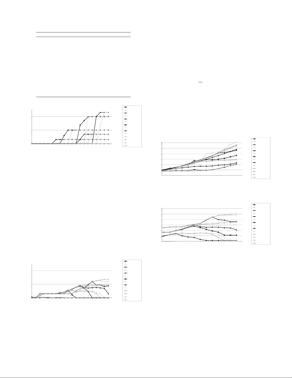
Uni v ersal Approximation of Edge Density in Lar ge Graphs Marc Boull ´ e Orange Labs 22300 Lannion, France Email: marc.boulle@orange.com Abstract —In this paper , we present a novel way to summarize the structure of large graphs, based on non-parametric estimation of edge density in directed multigraphs. Following coclustering approach, we use a clustering of the vertices, with a piecewise constant estimation of the density of the edges across the clusters, and address the problem of automatically and reliably inferring the number of clusters, which is the granularity of the coclustering. W e use a model selection technique with data- dependent prior and obtain an exact evaluation criterion for the posterior probability of edge density estimation models. W e demonstrate, both theoretically and empirically , that our data-dependent modeling technique is consistent, resilient to noise, v alid non asymptotically and asymptotically behaves as an universal approximator of the true edge density in directed multigraphs. W e evaluate our method using artiﬁcial graphs and present its practical interest on real world graphs. The method is both robust and scalable. It is able to extract insightful patterns in the unsupervised learning setting and to provide state of the art accuracy when used as a pr eparation step for supervised learning . I . I N T RO D U C T I O N W ith the recent av ailability of much network data, such as world wide web, social networks, phone call networks, science collaboration graphs [1], [2], there is a renewed interest for the graph partitioning problem, especially for the automatic discov ery of community structures in large networks [3], [4], [5]. Beyond clustering approaches, coclustering approaches aim at summarizing the relation between two entities in a many-to-man y relationship. Such a relation can be represented as a graph, where the source and target vertices represent entities and the edges stand for relations between entities. A coclustering model pro vides a summary of a graph by grouping source vertices and target vertices. For example, in market analysis , the source v ertices of the graph represent customers, the target vertices represent products and there is one edge each time a customer has purchased a product. A coclustering model summarizes the dataset by grouping customers that hav e purchased approximately the same products and grouping products that hav e been purchased by approximately the same customers. Coclustering models have been applied to many other domains, such as information retrie val (the entities are documents and their words in a text corpus), web log analysis (cookies and their visited web pages), web structure analysis (web pages with hyper -links between them) or telecommuni- cation network (the call detail records stand for the edges in a call graph between a caller and a called party). All these real-world graphs are directed multigraphs, meaning that two entities may be linked by multi-edges. W e aim to summarize and discover insightful patterns in such graphs, using a method with the desired following properties: 1) Robustness, to avoid detecting spurious patterns in case of noisy data. 2) Non asymptotic validity , to be able to detect reliable patterns with as few data as possible. 3) Asymptotic con vergence to the true underlying dis- tribution when it exists. 4) Parameter less 1 , with no user parameters to set. 5) Scalable, to process large graphs. In this paper, we present a novel way of analyzing and summarizing the structure of large graphs, based on piecewise constant edge density estimation. W e apply data grid models [6] to graph data, where each edge is considered as a statistical unit with two variables, the source and target vertices. The objectiv e is to ﬁnd a correlation model between the two variables by the means of a data grid model, which in this case turns out to be a coclustering of both the source and target vertices of the graph. The cells resulting from the cross- product of the two clusterings summarize the edge density in the graph. The best correlation model is selected using the MODL approach [7], and optimized by the means of combinatorial heuristics with super -linear time comple xity . The MODL approach is an application of the Minimum Description Length (MDL) principle [8], specialized in the follo wing way: use of hierarchical prior uniform at each stage of the hierarchy of the model parameters, use of discrete model parameters that are data dependent and use of combinatorial optimization algorithm to ﬁnd the MAP (Maximum a Posteriori) model. Compared with our previous work that introduced data grid models [6], we suggest a new interpretation of these models as uni versal density estimators and apply them to directed multigraphs, with potential loops and multi-edges, by considering these graphs as distributions of edges with unknown density . W e also show that in our model selection approach, the ﬁnite data sample is modeled directly , with a data-dependent prior distrib ution of the model parameters: this provides a non-asymptotic v alidity of the method. Further- more, we demonstrate new fundamental results that prov e the consistency of the approach, with an asymptotic conv ergence to the true underlying distribution when it exists. Finally , we relate our method to existing approaches and present extensi ve comparative experiments. Throughout the paper, all 1 Parameter -less means that there are no user parameter or hyper-parameter to set and that the model parameters are automatically inferred during the training process. the experiments are performed on a W indows PC with Intel Xeon W3530 2.8 Ghz, using the Khiops 2 software for the graph coclusterings based on our approach. The rest of the paper is org anized as follows. Section II explores related work. Section III reformulates the MODL method for data grid models in terms of ﬁnite data sample modeling and applies it to graphs. Section IV introduces the problem of edge density estimation, demonstrates the asymp- totically consistency of the MODL approach, and provides experimental results regarding the con vergence rate. Section V points out the dif ferences between our approach and three alternativ e methods, using artiﬁcial datasets in controlled com- parativ e experiments. Section VI shows that our method can be used both for exploratory analysis and as a preparation step for supervised learning, using three real world datasets. Finally , Section VII giv es a summary and suggests future work. I I . R E L A T E D W O R K Many approaches aiming at summarizing and ﬁnding struc- tures in graphs have been proposed in the literature. In this section, we discuss several of these approaches and relate them to our approach. A. Graph clustering Many approaches hav e been studied for the problem of graph clustering, including hierarchical clustering, di visi ve clustering, spectral methods, random walk (for a survey , see [9], [10]). T o e valuate the quality of a clustering [11] re gardless of the cluster number , the modularity criterion [12] is no w widely accepted in the literature and has even been treated as an objecti ve function in clustering algorithms [13], [3]. This criterion aims to obtain dense clusters where the within-cluster edge density is signiﬁcantly above the expected edge density in case of random edges following the same verte x degree distribution. Actually , not all graphs follo w a cluster tendency [14], with a structure consisting of natural clusters. Y et, all clustering algorithms output a partition into clusters for any input graph. While the clustering setting is relev ant in many domains, our approach does not rely of such cluster tendency assumption and may hav e a wider range of application. This is illustrated experimentally in Section V -A. B. Blockmodeling More expressi ve graph models aim at searching a partition of both the source and target vertices into clusters, with different types of interaction between clusters. The cross- product of the two partitions of vertices form a partition of the edges into bloc ks or coclusters . This modeling approach is called blockmodeling and has been thoroughly studied for decades. In early approaches [15], [16], non-stochastic blocks are considered, with a focus on predeﬁned types of block patterns. The blockmodel is searched either indirectly using a (dis)similarity measure between pairs of vertices and then applying a standard clustering algorithm, or directly by optimizing an ad hoc function measuring the ﬁt of real blocks to the corresponding predeﬁned types of blocks. The limit of 2 Khiops is a general purpose data preparation and scoring tool av ailable as a sharew are at http://www .khiops.com, which implements the MODL approach described in Section III. these approaches is that they do not cope with the stochastic nature of many real world datasets. C. Stochastic blockmodeling Using the framew ork of the exponential family , stochastic blockmodels are introduced by Holland et al. [17], with blocks still speciﬁed a priori. The approach is extended by W asserman and Anderson [18] to the discovery of block structure and exploits a statistical criterion, e .g. likelihood function, optimized using the EM algorithm. The method of Snijders and No wicki [19] considers blockmodels where the edge probabilities depend only on the blocks to which the vertices belong. The considered models are limited to two blocks, and searched via maximum likelihood estimation using the EM algorithm for small graphs and via Bayesian Gibbs sampling for larger graphs. The blockmodels are broadened to an arbitrary number of blocks [20], and optimized via Monte Carlo Marko v Chain (MCMC) Bayesian inference. Karrer and Newman [21] propose to include the degree distribution of the vertices as a correction to the blockmodels in order to better ﬁt real world graphs. For a surve y on recent work on stochastical blockmodeling via maximum likelihood methods, see [22]. In the connected approach named “mix ed member- ship blockmodels” [23], the mixture models are approximated owing to variational methods, which of fer better scalability at the expense of approximating the objecti ve function. Non- parametric extensions of the stochastic blockmodeling ap- proach have also been considered. In [24], a Dirichlet process is exploited as a prior for partitions of any size, to cluster both the source and target vertices of a directed simple graph, where the edges within each block are generated according to a Bernouilli distrib ution. Still, hyper -parameters are required in these approaches, such as the concentration parameter in the Dirichlet process, which inﬂuences the expected number of clusters in the non-asymptotic regime. Our approach is closely related to non-parametric 3 stochasticl blockmodeling approaches. It differs from existing approaches on the main following points: it is not restricted to simple graphs, the model selection method exploits a MAP (maximum a posteriori) approach with an e xact analytical criterion, not a Bayesian approach aiming at approximating the posterior distrib ution of the models, it is parameter -less, with no user parameter to set, and it exploits scalable optimization heuristics. A comparati ve experiment with a statistical block modeling method is pre- sented in Section V -B. D. Coclustering A directed multigraph is fully described by its adjacency matrix, where each entry of the matrix contains the number of edges between a source vertex (in a ro w) and a target verte x (in a target). This is equiv alent to the contingency table between two categorical v ariables in a dataset. Such contingency tables can be summarized using coclustering methods. In the applied mathematics ﬁeld, the seminal work of [26] treats the problem of coclustering of a numerical matrix, by looking at a partition of the rows and columns of the matrix. In the data mining ﬁeld, in case of binary variables, this technique has been applied to the simultaneous partitioning of the instances into clusters and 3 Here, we use the term non-parametric like in [25] for models where the number of parameters is not ﬁxed and may gro w with the sample size. of the v ariables into groups of variables [27], with methods like [28] closely related to the stochastic blockmodeling approach. Coclustering has also been applied to the domain of gene expression data [29], [30] by minimizing the sum squared residue to approximate a numerical matrix. The method of [31] optimizes a minimum loss of information to summarize a binary distance, with an application to text mining. While most approaches require the number of row and column clusters as user parameters, the method of [32] is parameter -less, by directly optimizing the Goodman-Kruskal’ s τ measure of association between two categorical v ariables. Like the method of [32], our approach focuses on contingency tables containing frequency data and is parameter -less. Howe ver , our method, being fully re gularized, is both resilient to over -ﬁtting and able to approximate the true joint distribution when it exists. E. Minimum description length based methods In the method of [33], the MDL principle [8], [34] is employed for the inference of the whole set of blockmodel parameters, including the number of blocks, in case of directed simple graphs. Using a two-part scheme for encoding for the model parameters and the data given the model, a parameter - less regularized criterion is obtained, inheriting from the MDL method’ s resistance to ov er-ﬁtting. The criterion is optimized using a greedy top-do wn heuristic, by adding one cluster at a time from a single-cluster initial model, and optimizing each coclustering model by moving values across clusters. In [35], the MDL method of [33] is extended to the case of spatial data mining. The method of [36] is dedicated to undirected simple graph, and the objective function is optimized using simulated annealing. Follo wing these MDL methods, sev eral encoding schemes are explored in [37] in the case of undirected simple graph to study their resistance to over -ﬁtting. A fast multi- lev el algorithm is exploited to generate candidate partitions of the vertices of varying sizes, with a focus on the single versus multiple cluster question. The study shows that earlier approaches tend to over -ﬁt the data with more than one cluster in case of random graphs, especially in case of ske wed degree distribution of the vertices. The early method of [33], which applies to directed simple graphs, is the closest to our method. The main differences are that our method (1) can be applied to directed multigraph, (2) relies on an exact analytical criterion without an y asymptotic approximation (such as using empirical entropies to encode the data, like in previous MDL-based methods), (3) is v alid both in the non-asymptotic and asymp- totic case, and (4) exploits a bottom-up greedy optimization heuristic. The impact of these differences both on artiﬁcial and real-world datasets is assessed in Sections V -C and VI. F . Alternative binary matrix summarization appr oaches Other approaches have been proposed to extract patterns from binary datasets. For example, a tile [38] is a region of a database deﬁned by a subset of rows and columns with a high density of 1, and a collection of tiles constitutes a tiling. A tile is then closely related to one single dense cocluster , and a tiling to a coclustering, although the tiling is not a partition of the database. In [39], [40], the maximum entropy principle [41] is applied with row and columns marginals as prior information, leading to an interestingness measure of tiles and a method for extracting a tiling. In [42], the same framew ork is applied for extracting multi-relational patterns: by representing multi-relational data as a K-partite graph, ex- tracting complete connected subgraphs reduces to the problem of extracting tiles. Coclustering has also been extended by considering a hierarchy of coclustering, where each cocluster is itself partitioned into a set of sub-coclusterings. In [43], the MDL method of [33] is extended to ﬁnd such patterns automatically , whereas in [44], the problem is treated using the Mondrian process, a multidimensional generalization of the Dirichlet process. T iling has also been extended to hierarchies of tiling in [45]. In [46], a binary matrix is decomposed as a product of Boolean factor matrices; extending standard matrix factorization methods, the proposed approach allows a better interpretability of the extracted patterns. Compared with these alternativ e pattern extraction approaches in binary matrices, our method focuses on the problem of coclustering of a contingency matrix (or adjacency matrix of a directed multigraph), which is a matrix of counts. I I I . M O D L A P P RO AC H F O R G R A P H S Data grid models [6] have been introduced for the data preparation phase of the data mining process [47], which is a key phase, both time consuming and critical for the quality of the results. They allow one to automatically , rapidly and reliably ev aluate the class conditional probability of any subset of variables in supervised learning and the joint probability in unsupervised learning. Data grid models are based on a partitioning of the v alues of each v ariable into intervals in the numerical case and into groups of values in the categorical case. The cross-product of the univ ariate partitions forms a multiv ariate partition of the representation space into a set of cells. This multiv ariate partition, called the data grid, can be interpreted as a piecewise constant non-parametric estimator of the conditional or joint probability . The best data grid is searched using a MAP approach and efﬁcient combinatorial heuristics. The method is non-parametric in the statistical sense, since it does not rely on the assumption that the data are drawn from a given probability distribution. It is also parameter-less, since all the model parameters, which number grows with the sample size, are automatically inferred without any user parameter . A. Basic Notions of Graph Theory A graph G = ( V , E ) consists of a set V of vertices and a set E of pairs of vertices called edges. A graph is undirected if the edges are unordered pairs of vertices, and is directed if the edges are ordered. A loop is an edge from one vertex to itself. A graph is simple in case of at most one edge per pair of vertices, and is a multigraph otherwise. T wo vertices of an undirected graph are called adjacent if there is an edge connecting them. An edge is incident to its two vertices, called extremities. The degree of a verte x is the number of edges incident to it. In case of directed graph, the extremities of an edges are called the source and target vertices of the edge, the in-degree of a verte x v is the number of edges with target v , and the out-degree of v is the number of edges with source v . Graphs can be represented by their adjacency matrix, where each cell of the matrix contains the number of edges per pair of vertices. The adjacency matrix of simple graphs contain only binary values, and that of undirected graphs is symmetrical. Figure 1 displays an example of directed simple graph. Figure 2 displays a directed multigraph with self-loops, as well as it adjacency matrix and the in and out-degrees of each verte x. B. MODL Criterion for Graphs W e reformulate the data grid approach in the context of edge density estimation in directed multigraphs. As shown in Figure 1, a directed graph can be represented in a tabular format with two v ariables, source vertex and target vertex, and one line per edge described by its two vertices. W e can then apply the data grid models in the unsupervised setting to estimate the joint density between these two variables, which is the density of edges in the graph. In this section, we formulate the approach as a modeling of a ﬁnite data sample, where the model parameters aim to summarize the edge counts in the sample. A B F D E C G Source T arget A D A F B A B C B D D G F G G E Fig. 1. Directed simple graph and its tabular representation. Let S and T be a source and target set of vertices, with n S = | S | source v ertices and n T = | T | target vertices, and let G be a directed multigraph with m edges from S to T . Giv en S , T and m , our objecti ve is to provide a joint description of the source and target vertices of the edges in the graph. One simple way to describe the edges e xploits the tabular format shown in Figure 1, with the count of edges per pair (Source, T arget) of vertices. W e can also summarize the location of edges at a coarser grain by introducing clusters of source vertices and clusters of target vertices, and considering the number of edges per pair of source and target cluster (coclus- ter). Such a coclustering model provides a summary of the graph. The coarsest summary is based on one single cluster of vertices with just the total number of edges, whereas the ﬁnest summary exploits one cluster per vertex, with the number of edges per pair of v ertices. Coarse grained summaries tend to be reliable, whereas ﬁne grained summaries are more informativ e. The issue is to ﬁnd a trade-off between the informativeness of the summary and its reliability , on the basis of the granularity of the coclustering. For gi ven sets of source and tar get vertices S, T and a gi ven number of edges m (sample size), we exploit a family of graph coclustering models, formalized in Deﬁnition 1. Deﬁnition 1: A graph coclustering model is deﬁned by: • the numbers k S , k T of source and target clusters of vertices, • the partition of the n S source vertices into the k S source clusters, resulting in n S i vertices per cluster, 1 ≤ i ≤ k S , • the partition of the n T target v ertices into the k T target clusters, resulting in n T j vertices per cluster , 1 ≤ j ≤ k T , • the distribution of the m edges of the graph G on the k E = k S k T coclusters with edge counts { m S T ij } 1 ≤ i ≤ k S , 1 ≤ j ≤ k T per cocluster , • for each source cluster of v ertices i , 1 ≤ i ≤ k S , the distribution of the m S i. edges originating in source cluster i on the n S i vertices of the cluster , i.e. the out- degrees { m i. } 1 ≤ i ≤ n S per source verte x, • for each target cluster of vertices j , 1 ≤ j ≤ k S , the distribution of the m T .j edges terminating in target cluster j on the n T j vertices of the cluster , i.e . the in-degrees { m .j } 1 ≤ j ≤ n T per target vertex. T ABLE I. N OTA T I O N S, T source and target vertex sets n S = | S | number of source vertices n T = | T | number of target vertices G directed multigraph with edges from S to T m number of edges in G M graph coclustering model for giv en S, T , m k S , k T number of clusters of source and target vertices k E = k S k T number of coclusters of edges m S T ij number of edges for cocluster ( i, j ) m i. number of edges for source vertex i (out-degrees) m .j number of edges for target vertex j (in-degrees) n S i number of vertices in source cluster i n T j number of vertices in tar get cluster j m S i. number of edges originating in source cluster i m T .j number of edges terminating in target cluster j m ij number of edges for pair ( i, j ) of vertices This notation, summarized in T able I, is illustrated in Figure 2, where a directed multigraph is displayed with its adjacency matrix. A clustered version of this graph is presented in Figure 3, which results in a coclustering of its adjacency matrix. A B F D E C G A B C D E F G P A 0 1 0 0 0 0 0 1 B 0 0 1 0 0 0 1 2 C 0 0 1 0 0 0 1 2 D 0 1 0 0 1 0 0 2 E 0 0 1 0 0 0 1 2 F 0 0 0 0 2 0 0 2 G 0 0 1 0 0 0 1 2 P 0 2 4 0 3 0 4 13 Fig. 2. Directed multigraph and its adjacency matrix. The numbers m ij in the adjacency matrix are the numbers of edges for each pair of vertices (for example, two edges from F to E). The sums m i. on the right column are the out-degrees of the vertices, and the sums m .j on the bottom line are the in-degrees of the vertices. The total number of edges is on the bottom right corner of the adjacency matrix. W e assume that the numbers of edges m and of source and target vertices n S and n T are known in adv ance and we aim to model the m edges of G between these two sets of vertices. This setting is general enough to account for directed graphs, bipartite graphs and undirected graph, where each edge comes twice with the two directions. The family of models introduced in Deﬁnition 1 is com- pletely deﬁned by the numbers k S and k T of clusters, the partitions of vertices into clusters, the edge counts in each A B F D E C G S1 S2 T1 T2 T3 A D F B E C G P A 0 0 0 1 0 0 0 1 D 0 0 0 1 1 0 0 2 F 0 0 0 0 2 0 0 2 B 0 0 0 0 0 1 1 2 E 0 0 0 0 0 1 1 2 C 0 0 0 0 0 1 1 2 G 0 0 0 0 0 1 1 2 P 0 0 0 2 3 4 4 13 T1 T2 T3 P S1 0 5 0 5 S2 0 0 8 8 P 0 5 8 13 Fig. 3. Directed multigraph with two source and three target clusters. The adjacency matrix of the graph (reorganized by clusters) is presented on the top-left, and that of the clustered graph at the bottom. The numbers m S T ij in the clustered adjacency matrix are the numbers of edges for each cocluster (for example, 5 edges from S1 to T2). coclusters { m S T ij } 1 ≤ i ≤ k S , 1 ≤ j ≤ k T , and the out- and in-degree of each verte x { m i. } 1 ≤ i ≤ n S , { m .j } 1 ≤ j ≤ n T . The numbers of vertices per cluster n S i and n T j are deri ved from the speciﬁcation of the partitions of vertices into clusters: they do not belong to the model parameters. Similarly , the numbers of edges originating or terminating in each cluster can be deduced by adding the frequencies of coclusters, according to m S i. = P k T j =1 m S T ij and m T .j = P k S i =1 m S T ij . In order to select the best model, we apply a MAP approach. W e suggest the prior distrib ution of the model parameters described in Deﬁnition 2, by applying the follo wing modeling choices: use of discrete rather than real-valued distri- butions, of the “natural” hierarchy of the model parameters and choice of uniform distributions at each lev el of the hierarchy , to be as uninformativ e as possible. Deﬁnition 2: The prior for the parameters of a graph coclustering model are chosen hierarchically and uniformly at each lev el: • the numbers of clusters k S and k T are independent from each other , and uniformly distrib uted between 1 and n S for the source vertices, between 1 and n T for the target vertices, • for a given number k S of source clusters, e very parti- tion of the n S vertices into k S clusters is equiprobable, • for a giv en number k T of target clusters, e very parti- tion of the n T vertices into k T clusters is equiprobable, • for a model of size ( k S , k T ) , ev ery distribution of the m edges on the k E = k S k T coclusters is equiprobable, • for a giv en cluster of source (resp. target) vertices, ev ery distribution of the edges originating (resp. ter - minating) in the cluster on the vertices of the cluster is equiprobable. Finally , we no w introduce the notion of consistency of a graph coclustering model with a graph sample in Deﬁnition 3. Deﬁnition 3: For given sets of vertices S, T and number of edge m , a graph coclustering model M is consistent with a graph sample G if and only if the edge counts { m S T ij } , { m i. } , { m .j } in the model are exactly the same as the related empirical edges counts { M S T ij } , { M i. } , { M .j } in the graph sample. A model which is not consistent with the data cannot generate the data and obtains a null posterior probability . W e now focus on the posterior probability of consistent models to obtain the ev aluation criterion giv en in Theorem 1 [6]. Theor em 1: The ne gati ve log of the posterior probability of a graph coclustering model M consistent with a graph sample G , distributed according to a uniform hierarchical prior , is giv en by c ( M ) = log n S + log n T (1a) + log B ( n S , k S ) + log B ( n T , k T ) (1b) + log  m + k E − 1 k E − 1  (1c) + k S X i =1 log  m S i. + n S i − 1 n S i − 1  (1d) + k T X j =1 log  m T .j + n T j − 1 n T j − 1  (1e) + log m ! − k S X i =1 k T X j =1 log m S T ij ! (1f) + k S X i =1 log m S i. ! − n S X i =1 log m i. ! (1g) + k T X j =1 log m T .j ! − n T X j =1 log m .j ! (1h) B ( n, k ) is the number of divisions of n elements into k subsets (with potentially empty subsets). When n = k , B ( n, k ) is the Bell number . In the general case, B ( n, k ) can be written as B ( n, k ) = P k i =1 S ( n, i ) , where S ( n, i ) is the Stirling number of the second kind [48], which stands for the number of ways of partitioning a set of n elements into i nonempty subsets. Mainly , the ev aluation criterion of Theorem 1 relies on counting the number of possibilities for the model parameters and for the data gi ven the model. In Equation 1, line (1a) 4 relates to the prior distribution of the cluster numbers k S and k T and line (1b) 5 to the speciﬁcation of the partition of the source (resp. target) vertices into clusters. These terms are the same as in the case of the MODL supervised univ ariate value grouping method [49]. Line (1c) 6 represents the speciﬁcation of the parameters of the distrib ution of the m edges on the k E coclusters, followed in line (1d) (resp. line (1e)) by the speciﬁcation of the distribution of the edges originating (resp. terminating) in each cluster on the vertices of the cluster . Line 4 For the choice of an integer parameter k uniformly distrib uted between 1 and n , we get p ( k ) = 1 n , leading to − log k = log n . 5 For a partition of n elements into k subsets chosen unifomly among B ( n, k ) possibilities, we get log B ( n, k ) terms in the criterion. 6 The number of positi ve integer parameters ( n 1 , . . . , n k ) with P k i =1 n i = n is  n + k − 1 k − 1  . (1f) 7 stands for the likelihood of the distribution of the edges on the coclusters, by the means of a multinomial coefﬁcient. Finally , line (1g) (resp. line (1h)) corresponds to the likelihood of the distrib ution of the edges originating (resp. terminating) in each cluster on the vertices of the cluster . As negati ve log of probabilities are code lengths, our model selection technique is similar to a practical minimum descrip- tion length principle [8], [34] with two-part MDL code. Our method is valid non-asymptotically , since it directly encodes the edge counts of the data sample. The inferred MAP model is necessarily consistent with the data sample: it provides a valid summary of the edge counts in the graph sample, b ut without any asymptotic guarantee w .r .t. the underlying edge probability distribution. In Section IV, we study the asymptotic behavior of the approach as the number of edges in the data sample goes to inﬁnity , and demonstrate that it can be interpreted as an edge density estimator with asymptotic conv ergence to the true edge distribution when it exists. C. Optimization Algorithm Graph coclustering models are no other than data grid models [6] applied to the case of joint density estimation of the source and target vertices of the edges. The space of data grid models is so large that straightforward algorithms almost surely fail to obtain good solutions within a practicable computational time. Sophisticated heuristics are described in [6] to optimize the criterion c ( M ) . They ﬁnely exploit the sparseness of the adjacency matrix of the graph and the additivity of the criterion, and allo w a deep search in the model space with O ( m ) memory complexity and O ( m √ m log m ) time complexity . In this section, we give an overvie w of the optimization algorithms which are fully detailed in [6], and rephrase them using the graph terminology . The optimization of a data grid is a combinatorial problem. The number of possible partitions of n vertices is equal to the Bell number B ( n ) = 1 e P ∞ k =1 k n k ! . Even with very simple models having only two clusters of source and target vertices, the number of models inv olves 2 n S + n T coclusterings of the v ertices. An exhausti ve search through the whole space of models is unrealistic. W e describe in Algorithm 1 a greedy bottom up merge heuristic (GBUM) which optimizes the model criterion c ( M ) . The method starts with a ﬁne grained model, with few vertices per source or target cluster , up to the maximum model M Max with one verte x per source or target cluster . It considers all the mer ges between clusters (independently for the source and target sets of v ertices), and performs the best merge if the criterion decreases after the merge. The process is reiterated until no further merge decreases the criterion. Each ev aluation of the criterion for a model requires O ( n 2 ) time, since the initial model contains up to n S n T coclusters (see Equation (1)) in the case of the maximal model M Max . Each step of the algorithm relies on O ( n 2 ) ev aluations of merges of clusters of v ertices, and there are at most O ( n ) steps, since the model becomes equal to the null model M ∅ (one sin- gle cluster) once all the possible merges have been performed. Overall, the time comple xity of the algorithm is O ( n 5 ) using 7 The number of ordered partitions of n elements into k subsets of sizes ( n 1 , . . . , n k ) is given by the multionomial coef ﬁcient. Algorithm 1 Greedy Bottom Up Merge heuristic (GBUM) Require: M { Initial solution } Ensure: M ∗ , c ( M ∗ ) ≤ c ( M ) { Final solution with improved cost } 1: M ∗ ← M 2: while improved solution do 3: M 0 ← M ∗ 4: for all mer ge between two source or target clusters do 5: { Consider mer ge for model M ∗ } 6: M + ← M ∗ + mer ge 7: if c ( M + ) < c ( M 0 ) then 8: M 0 ← M + 9: end if 10: end for 11: if c ( M 0 ) < c ( M ∗ ) then 12: M ∗ ← M 0 { Improv ed solution } 13: end if 14: end while a straightforward implementation of the algorithm. Ho wever , the method can be optimized in O ( m √ m log m ) time. The optimized algorithm mainly exploits the sparseness of the data, the additivity of the criterion and starts from non-maximal models with pre and post-optimization heuristics. • Large graph are often sparse, with far less edges than in complete graphs. Although a model may contain O ( n 2 ) coclusters, at most m coclusters are non empty . Since the contribution of empty coclusters is null in the criterion 1, each ev aluation of a data grid can be performed in O ( m ) time owing to speciﬁc algorithmic data structures (mainly , sparse representation with fast access to edges via hash-index es). • The additivity of the criterion means that it can be decomposed on the hierarchy of the components of the models: extremity (sources vs target variable), cluster of vertices, cocluster . Using this additi vity property , all the merges between adjacent clusters can be e valuated in O ( m ) time. Furthermore, when the best mer ge is performed, the only impacted mer ges that need to be reev aluated for the next optimization step are the mer ges that share edges with the best mer ge. Since the graph is potentially sparse, the number of reev aluations of models is small on average. • Finally , the algorithm starts from initial ﬁne grained solutions containing at most O ( √ m ) clusters. Speciﬁc pre-processing and post-processing heuristics are e x- ploited to locally impro ve the initial and ﬁnal solutions of Algorithm 1 by mo ving v ertices across clusters. The post-optimization algorithms are applied alternatively to the source and target vertex variables, for a frozen partition of the other variable. This allo ws one to keep a O ( m ) memory complexity and to bound the time complexity by O ( m √ m log m ) . Sophisticated algorithmic data structures are necessary to exploit these optimization principles and guarantee a time complexity of O ( m √ m log m ) for initial solutions exploiting at most O ( √ m ) clusters of vertices. The optimized version of the greedy heuristic is time efﬁcient, but it may fall into a local optimum. This problem is tackled using the v ariable neighborhood search (VNS) meta- heuristic [50], which mainly beneﬁts from multiple runs of the algorithms with different random initial solutions. The main heuristic described in Algorithm 1, with its guaranteed time complexity , is used to ﬁnd a good solution as quickly as possible. The VNS meta-heuristic is exploited to perform anytime optimization: the more you optimize, the better the solution. T o fa vor quality ov er speed, the meta-heuristic default setting is to perform at least 10 rounds of the main optimization heuristic before stopping. The optimization algorithms summarized abov e have been extensi vely ev aluated [6], using a large variety of artiﬁcial datasets, where the true data distribution is known. Overall, the method is both resilient to noise and able to detect comple x ﬁne grained patterns. It is able to approximate an y data distrib ution, provided that there are enough instances in the train data sample. I V . C O N S I S T E N C Y O F T H E A P P RO AC H F O R E D G E D E N S I T Y E S T I M A T I O N In this section, we interpret the models presented in Sec- tion III as edge density estimators, demonstrate that the MODL approach con verges asymptotically to the true edge density distribution when it exists. W e also pro vide experimental results regarding the conv er gence rate of the approach. A. Edge Density Estimation In our approach, we consider the graphs as generative models, where the statistical units are the edges with two variables per edge, the source and target v ertices of the edge. Whereas most blockmodeling approaches deal with simple graphs, focusing on their topology with at most one edge per pair of vertices, we regard graphs as statistical distributions of directed edges, with potential loops and multi-edges. A graph edge density model for a set of n vertices is entirely deﬁned by a set of probability parameters { p ij } 1 ≤ i ≤ n, 1 ≤ j ≤ n , where p ij stands for the probability of each independent and identically distributed (i.i.d) edge having source vertex i and target vertex j . Giv en these settings, a graph G containing m edges is treated as a sample of size m drawn from the edge distribution. Therefore, large samples tend be produce complete graphs from a pure topological point of vie w , but with varying edge densities taking into account the generative model. This edge density model applies to much real world graph data. In web log analysis, it seems natural to consider a bipartite graph, with users as source vertices, web pages as target vertices and edges representing web navigation. A sample graph corresponds to an extract of web log data, with the popular pages much more seen than the others. In a phone call network, each edge represents one phone call from a caller verte x to a called vertex, so that two vertices can be connected by multi-edges. Collecting the phone calls during a gi ven time period corresponds to a sample of a directed multigraph, where the potential communities correspond to subgraphs with high multi-edge density . The case of undirected graphs can be treated with symmetrical edge probabilities and a pair of directed edges per undirected edge 8 . Giv en this random graph generative model, the problem is to estimate the edge densities in the graph from a ﬁnite data sample. Estimating the n 2 edge probability parameters p ij from a sample of size m is not an easy task, especially in the case of sparse graphs. B. MODL Appr oach for Edge Density Estimation In the following, we propose a ne w interpretation of our approach described in Section III and sho w how it reduces to a ﬁnite sample modeling, which asymptotically conv er ges to an estimation of the edge density parameters. Giv en a graph coclustering model M as deﬁned in Sec- tion III, let us introduce the following notation for the proba- bility of the edges in a coclustered random graph: • { p S T κλ } 1 ≤ κ ≤ k S , 1 ≤ λ ≤ k T : probability distribution of the edges falling in each cocluster ( κ, λ ) • { p κ,i. } k S ( i )= κ : probability distribution of the out- degrees of the v ertices i of the source cluster κ • { p λ,.j } k T ( j )= λ : probability distribution of the in- degrees of the v ertices j of the target cluster λ Using this notation, the probability parameters of a coclus- tered random graph can be empirically estimated from the edge count parameters in a model M according to: p S T κλ = m S T κλ m , p κ,i. = m i. m S κ. , p λ,.j = m .j m T .λ . (2) This is a piece-wise constant modeling of the edge density with respect to the coclusters, constrained by the distributions of the in and out-degrees of the vertices in each cluster . Assuming the independence between the source and target vertices of the edges inside each cocluster , we get the follo wing estimation of the edge densities: p ij = p S T κλ p κ,i. p λ,.j = m S T κj m m i. m S κ. m .j m T .λ , (3) where ( κ, λ ) is the cocluster containing the edge ( i, j ) . For the null model M ∅ with one single cluster ( κ = λ = 1 ), we hav e p S T 11 = 1 , p 1 ,i. = m i. m , p 1 ,.j = m .j m , p ij = m i. m m .j m , (4) which means that the joint probability distribution p ij is the product of the two independent marginal distributions of the in and out-degrees of the v ertices. For the maximal model M Max with one cluster per vertex, we hav e p S T ij = m ij m , p i,i. = 1 , p j,.j = 1 , p ij = m ij m , (5) which means that the joint probability distrib ution p ij of the edges is directly estimated by the model parameters. 8 Although our approach can deal with undirected graphs using both directions, such graphs would beneﬁt from a specialized prior (potentially very dif ferent) and from simpler optimization algorithms (no need for alternate optimization of the partitions, for example). C. Asymptotic Con ver gence of the MODL Appr oach The family of coclustered random graphs is very expres- siv e and can theoretically approximate any edge distribution provided that there is sufﬁcient data. The problem is to select the best model giv en the data. The MODL approach aims to model directly the ﬁnite data sample, and exploits a discrete model space of the edge counts in the sample graph. W orking on a set of parameters of ﬁnite size allows one to deﬁne a “natural” hierarchical prior with uniform distribution at each lev el of the hierarchy , as in Deﬁnition 2, and reduces to counting in this discrete model space. This data-dependent modeling technique leads to the criterion of Equation 1, which can be interpreted as the exact posterior probability of the sample graph gi ven the model (Bayesian interpretation), or the exact code length of the model parameters and edges gi ven the model (two-part MDL interpretation [8], [34]). Therefore, the criterion does not rely on empirical estimation of continuous-v alued parameters (such as probabilities or entropies), which are valid only asymptotically . W e now study whether for given sets of source and target vertices, this exact ﬁnite data sample modeling asymptotically conv erges towards the true edge density when it exists, as the edge number goes to inﬁnity . Let us ﬁrst recall some concepts from information theory . The Shannon entropy H ( X ) [51] of a discrete random variable X with probability distribution function p is deﬁned as: H ( X ) = − X x ∈ X p ( x ) log p ( x ) . (6) The mutual information of two random v ariables is a quantity which measures the mutual dependence of the two variables [51]; it v anishes if and only if they are independent. For two discrete variables X and Y , the mutual information is deﬁned as: I ( X ; Y ) = X x ∈ X X y ∈ Y p ( x, y ) log p ( x, y ) p ( x ) p ( y ) , (7) where p ( x, y ) is the joint probability distribution function of X and Y , and p ( x ) and p ( y ) are the marginal probability distribution functions of X and Y respectively . Let us consider edges as statistical instances, with two verte x variables V S and V T having n S and n T values, and two verte x cluster variables V M S and V M T having k S and k T values for a given coclustering model M . W e present in Theorem 2 an asymptotic approximation of the ev aluation criterion c ( M ) introduced in Equation 1. Theor em 2: The MODL ev aluation criterion (Equation 1) for a graph coclustring model M is asymptotically equal to m times the entropy of the source and target verte x variables minus the mutual entropy of the v ariables grouped. c ( M ) = m  H ( V S ) + H ( V T ) − I ( V M S ; V M T )  + O (log m ) . (8) Pr oof: See Appendix. As the criterion has to be minimized, this means that the method aims to select a coclustering model which maxi- mizes the mutual information between the two vertex cluster variables. Since the mutual information of two variables is not other than the Kullback-Leibler div ergence [51] between the joint probability distribution of two variables and their independent joint distrib ution, this means that the best selected coclustering tends to highlight contrasts between the two variables, being as far as possible from their independent joint distribution. W e no w present an important result in Theorem 3, which shows that the MODL approach asymptotically con ver ges tow ards the estimation of the true edge distrib ution, which is the joint distribution of the source and target vertex variables. Although the modeling technique is data-dependent (regarding the model space and the prior on the model parameters) and aims to model exactly the data sample with a discrete distribution of the sample edges on the vertices, not the true edge continuous-v alued probability distrib ution, this theorem demonstrates the consistency of the approach. Theor em 3: The MODL approach for selecting a graph coclustering model M asymptotically con verges to wards the true edge distribution, and the criterion for the best model M Best con verges to m times the entropy of the edge variable, which is the joint entropy of the source and target vertices variables. lim m →∞ c ( M Best ) m = H ( V S , V T ) . (9) Pr oof: See Appendix. As a corollary of Theorem 3, Theorem 4 states that the MODL approach allo ws one to estimate the mutual informa- tion between the source and target vertices variables. Theor em 4: The MODL approach for selecting a graph coclustering model M asymptotically con verges to wards the true edge distribution, and the criterion for the null model minus the criterion for the best model M Best con verges to m times the mutual entropy of the source and target vertices variables. lim m →∞ c ( M ∅ ) − c ( M Best ) m = I ( V S ; V T ) . (10) Let us recall that the mutual information I ( V S ; V T ) is null in case of independent source and target vertices, such as for Erd ˝ os-R ´ enyi random graphs [52]. Theorem 4 shows that for such graphs, the best selected model will be asymptotically the same as the null model (which actually represents the case of independence). Since the MODL approach is regularized, with prior terms in criterion c ( M ) that grows with the granularity of the clusters, we expect the approach to select the null model in case of independence, ev en in the non-asymptotic case. This expected beha vior is conﬁrmed experimentally in Section V. D. Experimental Con vergence Rate of the MODL Appr oach W e ha ve shown that although the MODL approach aims to model the data sample directly , it asymptotically con verges tow ards the true edge density . The assumption behind the MODL approach is that the non-parametric edge density estimation will beneﬁt from ﬁne tuned ﬁnite data-dependent model space and prior , so as to conv erge as fast and reliably as possible. 60 80 100 Clusters 0 20 40 1.E+02 1.E+03 1.E+04 1.E+05 1.E+06 Edges 1 1.5 2 Mutual information True Empirical Laplace MODL(LH) MODL 0 0.5 1 1.E+02 1.E+03 1.E+04 1.E+05 1.E+06 Edges Fig. 4. Conv ergence of the MODL approach on the random circular graph with 100 vertices: number of clusters and difference between the estimated and true mutual information I ( V S ; V T ) per edge number in the graph sample. This conv er gence rate is hard to analyze theoretically in the non-parametric setting, without any assumption regarding the true edge density . For example, in the simple case of a cluster-based graph, the adjacency matrix is block-diagonal and most of the edge probabilities are null. In this case, few parameters need to be estimated and the con ver gence is fast. In this section, we chose a more difﬁcult sample graph where the distribution of the edge probabilities is rather smooth with no cluster-based structure, unbalanced and ne ver null, and present an experimental study of the conv ergence rate of the approach. Let us introduce cir cular random graphs as directed multigraphs, where the n vertices lie equidistant on the unit circle at positions ( x i = cos 2 π i n , y i = sin 2 π i n ) . The Eu- clidian distance between two vertices i and j being d ij = p ( x i − x j ) 2 + ( y i − y j ) 2 , which we extend by continuity to d ( i, i ) = 2 n for self-loops, we deﬁne the probability of having an edge between two vertices in in verse proportion of their distance, according to: ∀ i, j, p ij = 1 /d ij P µ,γ 1 /d µγ . (11) In such a circular random graph, the largest edge probabil- ities (related to self-loops with d = 2 n ) are n times larger than the smallest ones (related to pairs of vertices on a diameter of the circle, with d = 2 ), with a continuous decrease of edge probabilities in in verse proportion to the distance of their extremities. In our e xperiment, we chose a circular random graph with n = 100 vertices and randomly generate edges from sample size varying from 100 to 10 6 . For each sample size, we run the MODL algorithm and collect both the number of clusters and the mutual information estimated according to the data grid edge probability estimator (see Equation 3) and to the MODL criterion (see Equation 10 from Theorem 4). For comparison purpose, we also report the true mutual information (kno wn exactly for this artiﬁcial dataset), as well as its empirical estimation (using p ij = m ij m ) and according to the Laplace estimator ( p ij = m ij +1 m + n 2 ). The experiment is repeated 100 times, so as to estimate both the mean and the standard deviation of the collected measures, presented in Figure 4. The empirical estimator tends to over -ﬁt the data (the mutual information is lar gely ov erestimated, especially for small sample sizes), whereas the Laplace estimator tends to under-ﬁt the data. In accordance with Theorem 4, the MODL criterion of Equation 10 con verges tow ards the true mutual information. The MODL(LH) criterion (likelihood terms only , without prior terms as in Equation 10) related to the best selected model exhibits a much faster con vergence rate, while not o ver -ﬁtting the data. Figure 4 shows three phases in the con vergence of the MODL approach. In the ﬁrst phase ( stability phase ), the number of edges is not sufﬁcient to reliably estimate the edge probabilities, and the approach ev aluates the random graph with one single cluster as being the most probable. In the second phase ( non-parametric estimation phase ), the method identiﬁes regularities in the graph by building clus- ters and approximating the true mutual information, with an increased accuracy as the sample size grows. In the third phase ( classical estimation phase ), the method has built one cluster per vertex and estimates all the n 2 edges probabilities simultaneously according to a classical empirical estimation of a set of multinomial parameters: the accuracy of the estimation “classically” increases with the sample size. In this example, the non-parametric estimation phase starts when the number of av ailable edges is about 500, about 1 20 of the number of edge probability parameters, and has conv erged at about 150,000 edges, ﬁfteen times the number of edge probability parameters. It is noteworthy that in most large real world graphs, the method will run in the non-parametric estimation phase. Overall, this experiment shows that the method is reliable, quickly discovers true regularities in the graph as soon as there is sufﬁcient data, and is able to approximate complex edge density distributions with a fast con ver gence rate. V . C O M PA R A T I V E E X P E R I M E N T O N A RT I FI C I A L D A TA S ET S In this section, with exploit artiﬁcial datasets, where the true edge distribution is kno wn, to compare our approach to alternativ e methods. W e ﬁrst relate our method to a graph clustering method, then to a statistical blockmodeling method, and ﬁnally to a parameter-less coclustering method based on MDL. A. Comparison with Graph Clustering This section, intended to be of a tutorial nature, points out the difference between graph clustering and our method, which exploits a coclustering approach. W e ﬁrst recall the modularity criterion which is widely used for graph clustering methods, then illustrate the difference between the approaches using artiﬁcial datasets. 1) Modularity Criterion for Graph Clustering Methods: The goal of community detection is to partition a network into clusters of vertices with high edge density , with the vertices belonging to different clusters being sparsely connected. T o ev aluate the quality of a partition, the modularity Q [12] is a widely used criterion in recent community detection methods. The modularity measures the density of edges inside clusters as compared to the one expected in case of independence of the vertices. Giv en a graph G with n vertices and m edges, let m ij be an element of the adjacency matrix of the graph. m ij = 1 if vertices i and j are connected by an edge, m ij = 0 otherwise. The degree of a verte x i is deﬁned by the number of edges incident upon it. In the case of undirected graphs, the ouput and input degree of a vertice are equal. Using the notation of Section III-B, we hav e m i. = m .i = X j m ij = X j m j i . (12) An undirected graph with m U edges corresponds to a symmetrical directed graph with m = 2 m U edges. Assuming that the verte x degrees are respected, the probability of a random edge between vertices i and j is m i. m .j /m 2 . The modularity Q is deﬁned as Q = 1 m X ij  m ij − m i. m .j m  δ ( k S ( i ) , k T ( j )) , (13) where k S ( i ) = k T ( i ) is the index of the cluster to which verte x i is assigned, the δ -function δ ( x, y ) is 1 if x = y and 0 otherwise and m = P ij m ij is twice the number of (undirected) edges. The modularity takes its values between -1 and 1 and has positi ve values when the clusters ha ve more internal edges that the expected edge number if connections where made at random, with the same vertex degrees. The value of this criterion is 0 in the two extreme cases of one single cluster and of as many clusters as vertices. The modularity criterion has two appealing properties: it is well founded for the discovery of clusters with a density higher than the expected density when the extremities of the edges are independent, and it does not require any parameter , such as the number of clusters. Modularity has been used to ev aluate the quality of par- titions for a large variety of methods such as hierarchical clustering, spectral clustering, random walks (see Section I), but also as an objecti ve function to optimize. In this section, we compare our approach with the state of the art Louvain method [3], which is v ery fast and b uilds high quality partitions (measured by the modularity criterion). 2) Artiﬁcial Graph F amily: W e introduce a family of artiﬁcial graphs consisting in four clusters of ten vertices, named A, B , C, D . F or two-dimensional depiction purpose, we consider the case of undirected simple graphs, with at most one edge per pair of vertices and no loops, and control the proportion of potential edges per cocluster , that is per pair of clusters of vertices. This is illustrated in Figure 5, where the four clusters of vertices are drawn on circles for better readability . For example, choosing a proportion p = 20% for the edges of ( A, B ) means that 20% of the potential edges with one extremity in A and the other one in B (among 100 = 10 ∗ 10 edges) are in the graph. In the rest of the section, we illustrate the dif ference between graph clustering and coclustering using two graph patterns: quasi-cliques and cocliques. 3) Quasi-cliques: Figure 5 presents a classical pattern con- sisting of four dense clusters, with an intra-cluster density of 80% and an inter-cluster density of 10% . The parameters of the edges distribution are shown on the left, then an example of a graph generated according to this distribution, and on the right the clusters retriev ed using our approach and the modularity- based approach, with a different color per cluster . The cluster based and coclustering methods (modularity method of [3] and our approach) obtain the same result, with a correct identiﬁcation of the four clusters related to A, B , C, D (with Q = 0 . 409 ). In the case of a graph that can be decomposed into dense clusters, the two approaches e xhibit the same behavior . Distribution Example Coclustering Graph clustering Fig. 5. Artiﬁcial graph: quasi-cliques. 4) Cocliques: Figure 6 presents a pattern consisting of four cocliques, which are subgraphs with no inner edge, and an edge density across cocliques of 50% . In this example, the intra-cluster density is far belo w the average density . Actually , not all graphs hav e a structure consisting of natural clusters. Y et, all clustering algorithms output a partition into clusters for any input graph, and the cluster based algorithm builds dubious clusters in this case. Our approach correctly retrie ves the four empty cocliques. In this case, the modularity is neg ativ e (- 0.251), which reﬂects the fact that the ratio between observed and expected edge density is far below 1. Distribution Example Coclustering Graph clustering Fig. 6. Artiﬁcial graph: cocliques. B. Comparison with Stochastic Blockmodeling In this section, we focus on the blockmodeling approach and report comparative e xperiments on two kinds of artiﬁcial graphs: blockmodel graphs and random graphs. 1) Blockmodel Gr aphs: Our method is a piece wise constant non-parametric edge density estimator in directed multigraphs. One of the closest existing approach is the statistical block- modeling one, and we used the StOCNET software for com- parison purpose. StOCNET [53] is a software system for the advanced statistical analysis of social networks, which imple- ments the stochastic blockmodeling method named BLOCKS of No wicki and Snijders [20], which applies to simple graphs. Although StOCNET requires the number of blocks as an input parameter , the tool can compute the blockmodeling structure for numbers of blocks between 2 and 8. The ﬁt of the block structure is e valuated using the clarity of the block structure [20]. The authors suggest to keep the model with the best ﬁt (smallest clarity) to select the best number of blocks. W e ev aluate the ability of the approach to retriev e the correct block structure using a graph consisting of 100 vertices with three clusters: 30 vertices in cluster A, 40 in cluster B and 30 in cluster C. The distribution of the edges across the clusters is summarized in T able V -B1, where the source and target vertices of each edge are uniformly distributed within each cluster . For each sample size 100, 200, ..., 1,000 edges, we generate one hundred datasets according to this edge distrib ution and run both the StOCNET software and our method with their default settings. The computation time of StOCNET is on average 210 seconds, while our methods takes on av erage 0.2 seconds. T ABLE II. A RT IFI C I A L B LO C K M OD E L D I S TR I B U TI O N W I T H T H RE E C L US T E R S . A B C P A 30% 0% 0% 30% B 0% 10% 30% 40% C 0% 30% 0% 30% P 30% 40% 30% 100.00% In Figure 7, we report the mean plus/minus the standard deviation of the selected block number, both for the StOCNET sofware and our approach. While the clarity criterion of StOCNET selects on a verage the correct number of clusters for suf ﬁciently large sample size, the selection approach is not resilient to sample variability . Our approach builds one single cluster for less than 200 edges and exactly three clusters beyond 600 edges, with a transition between 300 and 500 edges where two clusters (A versus B ∪ C) are sometimes selected. 1 2 3 4 5 0 200 400 600 800 1000 Number of clusters Edges StOCNET 1 2 3 4 5 0 200 400 600 800 1000 Number of clusters Edges MODL Fig. 7. Blockmodel graph: mean number of clusters per sample size, plus/minus the standard de viation This ﬁrst experiment shows that our method behaves as a blockmodeling approach w .r .t. the retrieved patterns. Being non-parametric, it beneﬁts from a regularized criterion to reliably estimate the correct granularity of the blockmodel pattern. 2) Random Graphs: The Erd ˝ os-R ´ enyi [52] random graph datasets used for tests were introduced by Johnson et al. [54]. These graphs are undirected simples graphs, that we treat as symmetric directed graphs with twice the number of edges in the adjacency matrix. The 16 available random graphs hav e verte x numbers 124, 250, 500 and 1,000, with av erage total degree 2.5, 5, 10 and 20. As StOCNET is limited to graphs with at most 200 v ertices, we could apply it only on the random graphs with 124 vertices. StOCNET takes 380 seconds on a verage on each 124 vertices graphs, while our method takes 0.4 second on a verage for these small graphs and up to 18 seconds for the largest graph with 1,000 vertices and 20,000 edges. On the 124 vertices graphs, for each average verte x degree, the clarity criterion of StOCNET signiﬁcantly decreases with the number of blocks, leading to the choice of maximum number of blocks considered (8 in the software). Using this criterion does not lead to a reliable choice of the block number in case of noisy data. Conv ersely , on all the random graphs up to 1,000 vertices and 20,000 edges, our method builds one single cluster , which conﬁrms its high resilience to noise. Overall, our method avoids the problem of parametric ap- proaches where the number K of clusters is a user parameter: it neither suffers from under-ﬁtting ( K too small) or o ver -ﬁtting ( K too large). C. Comparison with MDL Coclustering In this section, we compare our approach with the Cr oss- Association method [33]. As pointed out in Section II, this method is close to our approach: it performs a coclustering on (binary) matrices, is parameter-less and based on MDL, and is scalable, allowing experiments on large datasets. 1) Block-Diagonal Graphs: Let us introduce block- diagonal graphs as directed multigraphs with a partition of the source (resp. target) vertices into K clusters (chosen of equal size in this e xperiment), with edges lying in the related diagonal blocks. For each randomly chosen source vertex, an edge is generated randomly in the target cluster related to same block. In a noisy version of this pattern, edges are generated randomly among the whole graph with probability p , and according to the block-diagonal pattern with probability (1 − p ) . The contingency matrix of some samples of noisy block-diagonal graphs is drawn in Figure 8. Fig. 8. Sample of Noisy(100, 10), Noisy(1000, 5) and Noisy(1000, 100) block-diagonal graphs In the experiments, we use the same number of source and target vertices and consider the block-diagonal graphs described in T able V -C1. The Pure and Noisy graphs are block- diagonal graphs with a variety of number of v ertices and blocks, whereas the Random graphs reduce to Erd ˝ os-R ´ enyi random directed multigraphs. For all power of 2 sizes 1, 2, 4, 8, ... up to one million edges, we generate ten random graph samples according to the edge distribution of each artiﬁcial graph summarized in T able V -C1. W e run both the Cross- Association softw are 9 and our method with their default settings, and collect the mean cluster number and computation time. 2) Cluster Number: In Figure 9 and 10, we report the mean cluster number per sample size obtained with the MODL and Cross-Association methods for each artiﬁcial graph summa- rized in T able V -C1. For each graph, we observe three phases in Figure 9 for the MODL method, as in the experimental con ver gence study in Section IV -D: stability phase , with one single cluster , non-parametric estimation phase , with a gro wing number of clusters, and classical estimation phase , where the true cluster number is retrie ved. The second phase is very sharp for the 9 The Cross-Association software can be do wnloaded at http://www .cs.cmu.edu \ discretionary { - }{}{} /$ \ sim$deepay/mywww/ software/CrossAssociations- 01- 27- 2005.tgz. I am grateful to D. Chakrabarti for making his method av ailable and providing guidance in its use. T ABLE III. B L OC K - D IA GO N AL G RA P H S Name #V ertices #Blocks Noise rate Pure(10, 2) 10 2 0% Pure(100, 10) 100 10 0% Pure(1000, 5) 1000 5 0% Pure(1000, 100) 1000 100 0% Pure(10000, 200) 10000 200 0% Noisy(10, 2) 10 2 50% Noisy(100, 10) 100 10 50% Noisy(1000, 5) 1000 5 50% Noisy(1000, 100) 1000 100 50% Noisy(10000, 200) 10000 200 50% Random(10) 10 1 100% Random(100) 100 1 100% Random(1000) 1000 1 100% Random(10000) 10000 1 100% 100 Cluster nb Pure(10, 2) Noisy(10,2) Pure(100, 10) Noisy(100, 10) Pure(1000, 5) 10 Noisy(1000, 5) Pure(1000, 100) Noisy(1000, 100) Pure(10000, 200) Noisy(10000, 200) 1 1.E+00 1.E+01 1.E+0 2 1.E+03 1.E+04 1.E+05 1.E+06 Edge nb Random(10) Random(100) Random(1000) Random(10000) Fig. 9. Block-diagonal graphs: mean number of clusters per sample size using the MODL method block-diagonal graphs: belo w a threshold, which depends on the comple xity of the pattern (number of vertices and of blocks), only one cluster is retriev ed, and above about four times this threshold, the correct number of clusters is retrieved. The recognition threshold mainly increases with the number of vertices: simpler patterns require less edges to be identiﬁed, from 50 edges for the simplest Pure(10, 2) graph to 250,000 edges for the most complex Noisy(10000, 200) graph. In case of noisy data (with 50% noise), the shape of the curves is approximately the same, with a translation towards lar ger sample sizes: the noisy patterns require around four times the edge number necessary to retrieve the related pure patterns. Finally , the MODL method is highly resilient to noise: it never produces more cluster than expected, and always outputs one single cluster in the extreme case of random graphs. 100 Cluster nb Pure(10, 2) Noisy(10,2) Pure(100, 10) Noisy(100, 10) Pure(1000, 5) 10 Noisy(1000, 5) Pure(1000, 100) Noisy(1000, 100) Pure(10000, 200) Noisy(10000, 200) 1 1.E+00 1.E+01 1.E+0 2 1.E+03 1.E+04 1.E+05 1.E+06 Edge nb Random(10) Random(100) Random(1000) Random(10000) Fig. 10. Block-diagonal graphs: mean number of clusters per sample size using the Cross-Association method The results obtained by the Cross-Association method in Figure 10 are quite unclear . Still, this blurred behavior may be explained by the follo wing reasons. First, in case of pure patterns, the top-do wn algorithm can get stuck in local minima, resulting in an under-ﬁtting behaviour in case of patterns with many clusters. Second, in case of random patterns, as acknowledged in [33], the method tends to pick up spurious patterns and more generally to o ver -ﬁt the data. Last, the Cross- Association is designed for binary matrices related to directed simple graphs, not to directed multigraphs. Therefore, as any noisy multigraph is asymptotically ﬂattened to a complete simple graph, the Cross-Association method produces one single cluster for noisy patterns with many edges. 3) Computation T ime: The algorithmic complexity of the MODL method (main greedy bottom-up heuristic described in Algorithm 1) is O ( m √ m log m ) , where m is the number of edges. According to [33], the algorithmic complexity of the Cross-Association method is O ( m ( k ∗ + l ∗ ) 2 ) , where k ∗ and l ∗ are the number of source and target clusters retrieved by the top-down heuristic. Although this is quadratic w .r .t. the cluster number, this may be more ef ﬁcient that our bottom-up approach in case of patterns with small number of clusters. In Figure 11 and 12, we report the mean computation time per sample size obtained with the MODL and Cross-Association methods. 1000 10000 Time Pure(10, 2) Noisy(10,2) Pure(100, 10) Noisy(100, 10) Pure(1000, 5) 1 10 100 Noisy(1000, 5) Pure(1000, 100) Noisy(1000, 100) Pure(10000, 200) Noisy(10000, 200) 0.01 0.1 1.E+02 1.E+03 1.E+04 1.E+05 1.E+06 Edge nb Random(10) Random(100) Random(1000) Random(10000) Fig. 11. Block-diagonal graphs: mean computation time per sample size using the MODL method 1000 10000 Time Pure(10, 2) Noisy(10,2) Pure(100, 10) Noisy(100, 10) Pure(1000, 5) 1 10 100 Noisy(1000, 5) Pure(1000, 100) Noisy(1000, 100) Pure(10000, 200) Noisy(10000, 200) 0.01 0.1 1.E+02 1.E+03 1.E+04 1.E+05 1.E+06 Edge nb Random(10) Random(100) Random(1000) Random(10000) Fig. 12. Block-diagonal graphs: mean computation time per sample size using the Cross-Association method Compared to the theoretical computation complexity , the actual computation time depends on many factors, such as the numbers of vertices, the size of the true pattern and the lev el of noise. In the case of the MODL method (Figure 11), the shape of the computation time curve in the worse case is compliant with the theoretical complexity , with up to ten thousand seconds for the largest noisy graph. In the case of the Cross-Association method (Figure 12), the shape of the curves grows quadratically as expected, but is ﬂattened in the end with no more than one thousand seconds for the largest noisy graphs. This behavior comes from the bottom-up heuristic which is stuck in local minima and hardly produces more than around 20 clusters, which allows the method to be quicker at the expense of under -ﬁtting the data. Overall, whereas our method and the Cross-Association methods are both scalable, parameter-less and based on a similar MDL-based model selection approach, the modeling choices are quite dif ferent, resulting in contrasting behavior . Our method is valid both non-asymptotically and asymptoti- cally and neither suf fers from under-ﬁtting nor over -ﬁtting. It nev er produces spurious clusters in case of random graphs and recov ers complex patterns with an increased precision as the amount of av ailable data increases. V I . E X P E R I M E N T S O N R E A L W O R L D D A TA S E T S This section compares our method with the Cross- Association method [33] on real world datasets coming from three different domains: document clustering, webspam detec- tion and exploratory analysis of a ﬂight trip dataset. A. Document Dataset W e exploit the CLASSIC3 document dataset 10 introduced in [31] to e valuate the Information-Theoretic Coclustering ITC method. This collection of documents comes from three domains: MEDLINE consists of 1,033 abstracts from medical journals, CISI consists of 1,460 abstracts from information retriev al papers and CRANFIELD consists of 1,398 abstracts from aerodynamic systems. Overall, this dataset can be rep- resented as a directed multigraph with 3,891 source vertices (documents), 5657 target vertices (words) and 287,827 edges (184,772 edges in a ﬂattened binary representation of the graph). W e build a coclustering of the dataset using the MODL method described in Section III. The running time is one hour and 50 minutes. W e obtained a v ery ﬁne-grained summary of the dataset, with 151 clusters of documents and 293 clusters of word. Agglomerative hierarchical clustering method: In order to explore the coclustering at different granularities, we suggest to coarsen the obtained coclustering by the mean of an agglomerative hierarchical clustering. W e use the following similarity between two clusters i and j δ ( i, j ) = c ( M i ∪ j ) − c ( M ) , = log p ( M | G ) p ( M i ∪ j | G ) . (14) where c ( M ) is the ev aluation criterion (1) introduced in Section III, M is the current coclustering model and M i ∪ j is the coclustering model after the merge of clusters i and j . Intuitiv ely , if two clusters are similar , the total code length of the data (see criterion c ( M ) ) is not much different between the cases where the clusters are coded jointly or separately , so that δ will be small. Actually , the agglomerative hierarchical clustering algorithm is the same as that of Algorithm 1, except that the merges are performed until the required number of clusters is obtained. As the CLASSIC3 dataset comes from three domains, we chose to coarsen our ﬁne-grained 151 ∗ 293 coclustering matrix down to a 3*3 coarse matrix. The ﬁne and coarse grained matrix are shown in Figure 13. 10 Dataset available at http://www .dataminingresearch.com/index.php/2010/ 09/classic3- classic4- datasets/ Fig. 13. Coclustering of the CLASSIC3 dataset: initial ﬁne-grained 151 ∗ 293 coclustering matrix and coarse 3 ∗ 3 matrix. Applying the Cross-Association CA method, we obtain a 20*20 summary of the ﬂattened binary dataset in about six minutes. W e ev aluate the agreement between the coclustering results and the known documents classes for the MODL and CA methods: • MODL: we exploit the coarse 3*3 matrix to correlate the three obtained clusters of document with the known documents classes, • CA: we collect the majority class in each obtained cluster of document and manually group the clusters sharing the same majority class, do wn to three clus- ters. The results are reported in Figure 14. In [31], the ITC method is applied with three clusters as a user parameter , and obtains a good agreement between the retrie ved clusters and the true classes, with about 60 agreement errors. The CA methods obtain a better agreement than the ITC method, with about 20% less errors. The results are better for the MODL method with twice less agreement errors than for the CA method. MODL MED CISI CRAN P C1 1025 2 0 1027 C2 5 1446 0 1451 C3 3 12 1398 1413 P 1033 1460 1398 3891 CA MED CISI CRAN P C1 1014 9 3 1026 C2 17 1450 16 1483 C3 2 1 1379 1382 P 1033 1460 1398 3891 Fig. 14. CLASSIC3: agreement with the true classes for the MODL and CA methods. Overall, the MODL method produces a ﬁner coclustering than the CA method, at the expense of a a higher computation time. This ﬁner model better ﬁts the data, with a better agreement with the true classes in the dataset. B. W eb Spam Dataset In this section, we ev aluate the beneﬁt of our method as a preprocessing step for web spam detection. 1) W eb Spam Challenge 2007: W eb spam consists in manipulating the rele v ance of resources indexed in a manner inconsistent with the purpose of the indexing system of internet search providers. The data used in this paper comes from the W eb Spam Challenge (corpus #1, Track II) 11 held in conjunction with the 2007 ECML/PKDD Graph Labeling 11 http://webspam.lip6.fr/, W eb Spam Challenge 2007 workshop. The goal of the challenge is to ev aluate machine learning methods to label web hosts to be spam or normal. The data consists of 9,072 web hosts with both content and link data. Content data correspond to the TF-IDF vectors o ver 100 web pages of the host, with almost 5 millions features. The hosts are the vertices and the link data represent the edges in the directed host graph, with one edge per hyperlink between two hosts. Overall, the host graph contains 514,700 edges, all of them are simple edges. The degrees of the vertices follow the power -law distribution, as shown in Figure 15. The training set consists of 907 hosts labelled as normal or spam, with approximately 20% spam. The objective of the challenge is to label the test set (8,165 hosts). The result is assessed using the area under the R OC curve (A UC). 1 10 100 1 000 10 000 1 10 10 0 1000 10000 count degree Fig. 15. W ebspam challenge host graph: number of vertices per output de gree. The results of the challenge participants. 12 are reported on the right of Figure 17. They all used both the content and link data in a semi-supervised learning setting, on top of classiﬁers among which SVM, random forests and naiv e Bayes. All the av ailable data is exploited to build a model: train and test content and link data, plus the train labels. The link data is exploited either by extracting link-based features, such as number (or ratio) of links from (or to) to spam or normal hosts, or by constraining the classiﬁer to account for the labels of the connected hosts. 2) Evaluation: In a ﬁrst step, we exploit the link data only , that is the directed graph consisting of 9,072 hosts with 514,700 links. All the hosts and links are processed without any output label, to identify the “natural” clusters of source and target hosts. W e build a coclustering of the source and target hosts using the MODL method described in Section III. The running time is 3 hours and 14 minutes. The coclustering of the host graphs retrie ves 167 clusters of source hosts and 219 clusters of tar get hosts. The coclustered matrix is displayed in Figure 16, which shows that the graph of hosts is highly structured, with most of the information lying in few hundred of coclusters. The asymmetry in the hyperlinks of the host graph conforms to the observation of the challenge participants, that there is usually no link from a normal host to a spam host. Applying the alternativ e Cross-Association method, we ob- tain a 10*10 coclustering of the dataset in about ﬁ ve minutes. In a second step, the av ailable labeled train hosts are used to describe the output distrib ution in each cluster of hosts. The label of a test host is then predicted according to the output distribution of its cluster . Ho we ver , the MODL coclustering is ﬁne grained, and about 20% of the clusters do not contain 12 A vailable at http://airweb.cse.lehigh.edu/2008/web spam challenge/ introduction.pdf. Computation time of the participants is not av ailable. Fig. 16. Coclustering of the host graph of the web spam challenge. a single train instance: in this case the test host is labeled as the majority class (normal). T o alle viate this problem, we chose to coarsen our coclustering at dif ferent grain levels with the agglomerativ e hierarchical clustering method described in Section VI-A. W e build three new coarsened coclusterings, starting from the initial 386 = 167 + 219 clusters down to 200, 100 and 50 clusters. Giv en this preprocessing, each host is represented by eight v ariables, source or tar get cluster at four grain le vels. On the left of Figure 17, we report the test A UC obtained by each univ ariate cluster-based classiﬁer for the MODL coclustering ( S. clust( k ) and T . clust( k ) for classiﬁers based on source or target clusters for coclusterings with k clusters). W e also combined these classiﬁers using a Naive Bayes (NB) and a Selective Naiv e Bayes (SNB) classiﬁer [55]. Using the same protocol, we report the test A UC results obtained using the 10 times 10 coclustering retrieved by the Cross-Association method on the center of Figure 17. Finally , we also report the results of the challenge participants on the right of Figure 17. The test A UC results are obtained using the predeﬁned train/test split of the dataset to allow a comparison with the challenge participants. No cross-validation results are av ailable for the challenge participants. Given that the size of the test set is s = 8165 , the expected variance of the results is around 1 √ s ≈ 1% . T est AUC MODL result CA results Challenge results 1 M O D L r e s u l t C h a l l e n g e r e su l t s 0.95 0.9 0 . 9 5 0 . 8 5 0.9 0.85 0.8 0.75 0 . 7 0.75 0.7 Fig. 17. W ebspam 2007, phase II: test A UC results for the MODL and CA methods, and of the challenge participants. The Cross-Association method under-ﬁts the data, with an insufﬁcient number of clusters to correctly identify the spam class. For both the MODL and CA methods, the results show that the target clusters are much more informati ve than the source clusters, with 5 to 10% better test A UC. The granularity of the coclustering has a medium impact on the MODL test A UC: the best results is obtained with about 200 clusters. The combined classiﬁers manage to exploit all the input variables to get superior performance. It is note worthy that the (MODL) SNB classiﬁer obtains a test A UC comparable to that of the winner of the challenge, while using the link data only . Like in the document clustering experiment, the MODL method produces a ﬁner coclustering than the CA method, at the expense of a a higher computation time. This ﬁner model better ﬁts the data, with competitiv e performance for the task of web spam prediction. C. Flight T rip Dataset In this section, we apply our method on a large passenger ﬂight trip dataset for the purpose of exploratory analysis, when no ground truth is a vailable. The dataset 13 comes from the US Bureau of Transportation Statistics and contains a 10% sample of all airline tickets for each domestic ﬂight trip. W e collected the origin and destination ﬁelds as well as the number of passengers per trip for the four terms of year 2010, so as obtain 10% of all US domestic passenger ﬂight trips for one full year . The resulting data table contains 22,038,685 records, for a total of 469 airports and 43,092,916 ﬂight trips. The airports are the vertices and the trips are the oriented multiple edges from origin to destination airports. The average edge multiplicity in this graph is 471, with 91,482 different edges. W e apply the MODL coclustering method on this dataset, with a running time of 16 minutes 40 seconds. W e obtain a quasi symmetric summary of the multigraph with 233 clusters of origin airports, 234 clusters of destination airports, and 46,325 non empty coclusters. T ABLE IV . U S FLI G H T T R IP S AN D TH E I R C O C LU S T ER I N G S U M MA RY . PI WC FL D V CE P PI 1.03% 0.92% 0.03% 0.09% 0.49% 2.56% WC 0.89% 17.60% 1.79% 3.64% 10.54% 34.46% FL 0.03% 1.69% 0.30% 2.74% 6.15% 10.91% D V 0.09% 3.77% 3.13% 0.36% 6.41% 13.76% CE 0.28% 11.06% 5.60% 6.31% 15.07% 38.32% P 2.32% 35.04% 10.85% 13.14% 38.66% 100.00% In order to explore the extracted coclustering with a broader picture, we chose to coarsen our coclustering with the agglomerativ e hierarchical clustering method described in Section VI-A. For depiction purpose, we keep ﬁv e clusters: the coclustering matrix summary is almost symmetric, as shown in T able VI-C. Figure 18 displays the ﬁ ve clusters of destination airports. There is a clear geographic correlation in the clusters. A ﬁrst cluster consists of the Paciﬁc Islands (PI), with Haw ai, Mariana Islands, Guam and Samoa. A second cluster roughly corresponds to the Delaware V alley (DV), with counties from Pennsylvania, New Jersey , Delaware and Maryland. A third cluster contains the Florida airports (FL), while the two last clusters correspond the W est Coast (WC) and Center and East (CE) of America. Interestingly , the Paciﬁc Islands cluster is very dense, with 17 times more intra-cluster ﬂight trips than expected 13 http://www .transtats.bts.gov/DataIndex.asp, Airline Origin and Destina- tion Survey (DB1B) 2010, RIT A: Bureau of T ransportation Statistics Fig. 18. US ﬂight trips: ﬁve clusters of airports. in case of independence of the origin and destination of the trips ( 1 . 03% ≈ 17 ∗ (2 . 56% ∗ 2 . 32%) ). On the contrary , the Florida and Delaware V alley clusters are sparse clusters, with respectiv ely four times and ﬁ ve times less intra-cluster trips than expected in case of independence. Although these two sparse clusters are not geographically connected, they are linked by twice the number of trips than expected. This kind of exploratory analysis can be performed at any granularity up to the ﬁnest coclustering retriev ed by our method. This illustrates ho w the MODL coclustering method can be used for the task of exploratory analysis, when no ground truth is av ailable. V I I . C O N C L U S I O N In this paper , we hav e presented a novel w ay of discovering structures in graphs, by considering graphs as generative models whose statistical units are the edges, with unknown joint density of the source and target vertices. Our method applies the MODL approach based on data grid models [6] to the case of directed multigraphs. By clustering both the source and target vertices of a graph, the method behav es as a non-parametric estimator of the unknown edge density . The modeling approach exploits the MDL principle in a data- dependent way: it aims to model the ﬁnite graph sample directly . The modeling task is then easier, with ﬁnite modeling space and model prior which essentially reduce to counting. This modeling approach is both non-asymptotic and consistent, with an asymptotic con vergence towards the true edge density , without any assumption re garding this density . Experiments on artiﬁcial data demonstrate that our ap- proach is both robust, building one single cluster in case of random graphs, and accurate, being able to recov er ﬁne grained patterns. Our method has been applied to a document classiﬁcation problem and to a W eb spam detection problem in a graph of hosts. The patterns retriev ed by our approach are highly informative, with a good agreement with the true classes. An application on a large ﬂight trip dataset shows the potential interest of our method for exploratory analysis, with the extraction of insightful and interpretable patterns. Our method has a O ( m √ m log m ) time complexity , where m is the number of edges, providing practical running times up to millions of edges. In future work, we plan to work on faster and more scalable optimization algorithms in order to deal with very lar ge graphs, up to billions of edges. A P P E N D I X A P P E N D I X A. Pr oof of theor ems In this appendix we prove theorems 2 and 3 from Sec- tion IV -C. Theorem 2 The MODL evaluation criterion (Equation 1) for a graph coclustering model M is asymptotically equal to m times the entr opy of the sour ce and targ et vertex variables minus the mutual entr opy of the variables gr ouped. c ( M ) = m  H ( V S ) + H ( V T ) − I ( V M S ; V M T )  + O (log m ) . Pr oof: According to Equation 1, we have: c ( M ) = log n S + log n T (15a) + log B ( n S , k S ) + log B ( n T , k T ) (15b) + log  m + k E − 1 k E − 1  (15c) + k S X i =1 log  m S i. + n S i − 1 n S i − 1  (15d) + k T X j =1 log  m T .j + n T j − 1 n T j − 1  (15e) + log m ! − k S X i =1 k T X j =1 log m S T ij ! (15f) + k S X i =1 log m S i. ! − n S X i =1 log m i. ! (15g) + k T X j =1 log m T .j ! − n T X j =1 log m .j ! (15h) W e study the asymptotic beha vior of the criterion when the number of edges gro ws to inﬁnity , for a ﬁx ed set of vertices. Lines (15a) and (15b) of criterion c ( M ) are bounded by constants w .r .t. m . Since the numbers of clusters ( k S , k T ) and the numbers of vertices per cluster ( n S i , n T j ) are bounded by the number of vertices ( n S , n T ), lines (15c), (15d) and (15e) of the criterion, corresponding to the encoding of the model prior parameters, are bounded by O (log m ) . W e now focus on the likelihood terms of the criterion (lines (15f), (15g) and (15h). Using the approximation log n ! = n (log n − 1) + O (log n ) based on Stirling’ s formula and rearranging the terms with new m log m terms, we get: c ( M ) =   m log m − k S X i =1 k T X j =1 m S T ij log m S T ij   − m log m − k S X i =1 m S i. log m S i. ! −   m log m − k T X j =1 m T .j log m T .j   + m log m − n S X i =1 m i. log m i. ! +   m log m − n T X j =1 m .j log m .j   + O (log m ) . (16) Giv en that the sum of the edge counts in each partition (per cocluster , per cluster in and out-degree and per v ertex in and out-degree) is alw ays equal to m , we obtain: c ( M ) = − m k S X i =1 k T X j =1 m S T ij m log m S T ij m + m k S X i =1 m S i. m log m S i. m + m k T X j =1 m T .j m log m T .j m − m n S X i =1 m i. m log m i. m − m n T X j =1 m .j m log m .j m + O (log m ) . (17) As the marginal distributions m S i. and m T .j can be decom- posed by summation on the joint distribution m S T ij , we hav e: c ( M ) = − m k S X i =1 k T X j =1 m S T ij m log m S T ij m m S i. m m T .j m − m n S X i =1 m i. m log m i. m − m n T X j =1 m .j m log m .j m + O (log m ) . (18) Considering that the empirical estimation asymptotically con verges towards the related probabilities, the claim follo ws. Theorem 3 The MODL appr oach for selecting a graph co- clustering model M asymptotically conver ges towards the true edge distribution, and the criterion for the best model M Best con verg es to m times the entr opy of the edge variable, which is the joint entr opy of the source and tar get vertices variables. lim m →∞ c ( M Best ) m = H ( V S , V T ) . Pr oof: Using Theorem 2, we have c ( M ) = − mI ( V M S ; V M T ) + mH ( V S ) + mH ( V T ) + O (log m ) . W e apply the Data Processing Inequality (DPI) [51], which states that post-processing cannot increase information. More precisely , the DPI applies for three random variables X, Y , Z that form a Markov chain X → Y → Z . It means that the conditional distribution of Z depends only on Y and is conditionally independent of X . More speciﬁcally , for three random v ariables such that p ( Z | X , Y ) = P ( Z | Y ) , the DPI states that I ( X ; Y ) ≥ I ( X ; Z ) W e apply the DPI to the variables V S , V T , V M T . As the verte x cluster variable V M T can be computed according to a partition of the vertex variable V T ( V M T = f ( V T ) ), we hav e p ( V M T | V S , V T ) = p ( V M T | V T ) and thus obtain: I ( V S ; V T ) ≥ I ( V S ; V M T ) . (19) W e apply again the DPI to the variables V M T , V S , V M S . As the vertex cluster variable V M S is a function of V S , we have p ( V M S | V S , V M T ) = p ( V M S | V S ) and get: I ( V M T ; V S ) ≥ I ( V M T ; V M S ) . (20) By transitivity and since the mutual information is sym- metrical, we get: I ( V S ; V T ) ≥ I ( V M S ; V M T ) . (21) It is note worthy that this result applies to compare any pair of coclustering models, one of the models being a sub- partition of the other: the ﬁner model brings a higher mutual information. The model selection approach corresponds to a minimiza- tion of the MODL criterion. Let us now sho w that the best selected model asymptotically tends to be ﬁner and ﬁner, until reaching the ﬁnest possible model with one cluster per verte x, which is the maximal model M Max that enables a direct estimation of the edge probabilities p ij : I ( V S ; V T ) = I ( V M Max S ; V M Max T ) ≥ I ( V M S ; V M T ) . (22) If ∀ M , I ( V M Max S ; V M Max T ) = I ( V M S ; V M T ) , then using Theorem 2, the MODL approach asymptotically con ver ges tow ards the true edge distribution. If ∃ M f , M c , I ( V M Max S ; V M Max T ) = I ( V M f S ; V M f T ) > I ( V M c S ; V M c T ) , with M f a ﬁne-grained model having the same mutual information as the maximal model and M c a coarse-grained model, then let us sho w that the approach asymptotically selects the ﬁne-grained model M f rather than the coarser model M c . Let  = I ( V M f S ; V M f T ) − I ( V M c S ; V M c T ) 2 . Using Theorem 2 for the conv ergence of the criterion for model M c , ∃ m 1 , ∀ m ≥ m 1 ,     c ( M c ) m −  H ( V S ) + H ( V T ) − I ( V M c S ; V M c T )      <  2 . Similarly , for model M f , ∃ m 2 , ∀ m ≥ m 2 ,     c ( M f ) m −  H ( V S ) + H ( V T ) − I ( V M f S ; V M f T )      <  2 . Thus, ∀ m ≥ max( m 1 , m 2 ) , c ( M c ) m > H ( V S ) + H ( V T ) − I ( V M c S ; V M c T ) −  2 , c ( M f ) m < H ( V S ) + H ( V T ) − I ( V M f S ; V M f T ) +  2 . ∀ m ≥ max( m 1 , m 2 ) , c ( M f ) m − c ( M c ) m < I ( V M c S ; V M c T ) − I ( V M f S ; V M f T ) + , c ( M f ) m < c ( M c ) m − . Since the model selection approach corresponds to a min- imization of the MODL criterion, this means that the best selected model M Best asymptotically tends to be a ﬁne-grained model M f having the same mutual information as the maximal model M Max , which allows the estimation of the true edge distribution. Using Theorem 2 with the maximum model (limit of the best selected model), we hav e: c ( M Max ) = − mI ( V S ; V T ) + mH ( V S ) + mH ( V T ) + O (log m ) . As I ( X ; Y ) = H ( X ) + H ( Y ) − H ( X , Y ) , the claim follows. R E F E R E N C E S [1] R. Albert and A.-L. Barab ´ asi, “Statistical mechanics of complex net- works, ” Rev . Mod. Phys. , vol. 74, pp. 47–97, 2002. [2] C. Aggarwal and H. W ang, Eds., Managing and Mining Graph Data , ser . Adv ances in Database Systems. Springer, 2010, vol. 40. [3] V . Blondel, J.-L. Guillaume, R. Lambiotte, and E. Lefebvre, “Fast unfolding of communities in large networks, ” Journal of Statistical Mechanics: Theory and Experiment , vol. 2008, no. 10, p. P10008, 2008. [4] J. Leskov ec, K. Lang, A. Dasgupta, and M. Mahoney , “Community structure in large networks: Natural cluster sizes and the absence of large well-deﬁned clusters, ” Internet Mathematics , vol. 6, no. 1, pp. 29–123, 2009. [5] R. Jin, L. Liu, and C. Aggarwal, “Discovering highly reliable subgraphs in uncertain graphs, ” in KDD’11 , 2011, pp. 992–1000. [6] M. Boull ´ e, “Data grid models for preparation and modeling in su- pervised learning, ” in Hands-On P attern Recognition: Challenges in Machine Learning, volume 1 , I. Guyon, G. Cawley , G. Dror, and A. Saffari, Eds. Microtome Publishing, 2011, pp. 99–130. [7] ——, “MODL: a Bayes optimal discretization method for continuous attributes, ” Machine Learning , vol. 65, no. 1, pp. 131–165, 2006. [8] J. Rissanen, “Modeling by shortest data description, ” Automatica , vol. 14, pp. 465–471, 1978. [9] S. Schaeffer , “Graph clustering, ” Computer Science Review , vol. 1, no. 1, pp. 27–64, 2007. [10] S. Fortunato, “Community detection in graphs, ” Physics Reports , vol. 486, no. 3-5, pp. 75–174, 2010. [11] H. Almeida, D. Guedes, W . M. Jr ., and M. Zaki, “Is there a best quality metric for graph clusters?” in 15th European Conference on Principles and Practice of Knowledge Discovery in Databases , vol. 1, 2011, pp. 44–59. [12] M. Newman and M. Girvan, “Finding and ev aluating community structure in networks, ” Physical Review E , vol. 69, 2003, 026113. [13] A. Clauset, M. Newman, and C. Moore, “Finding community structure in very large networks, ” Physical Review E , vol. 70, no. 6, 2004, 066111. [14] J. Bezdek and R. Hathaway , “V at: a tool for visual assessment of (clus- ter) tendency , ” in International Joint Conference of Neural Networks , 2002, pp. 2225–2230. [15] F . Lorrain and H. White, “Structural equiv alence of individuals in social networks, ” J ournal of Mathematical Sociology , vol. 1, pp. 49–80, 1971. [16] P . Arabie, S. Boorman, and P . Levitt, “Constructing blockmodels: Ho w and why , ” Journal of Mathematical Psyc hology , vol. 17, no. 1, pp. 21– 36, 1978. [17] P . Holland, K. Laskey , and S. Leinhardt, “Stochastic blockmodels: First steps, ” Social Networks , vol. 5, no. 2, pp. 109–137, 1983. [18] S. W asserman and C. Anderson, “Stochastic a posteriori blockmodels: Construction and assessment, ” Social Networks , vol. 9, no. 1, pp. 1–36, 1987. [19] T . Snijders and K. No wicki, “Estimation and prediction for stochastic blockmodels for graphs with latent block structure, ” Journal of Classi- ﬁcation , vol. 14, no. 1, pp. 75–100, 1997. [20] K. No wicki and T . Snijders, “Estimation and prediction for stochas- tic blockstructures, ” Journal of the American Statistical Association , vol. 96, no. 455, pp. 1077–1097, 2001. [21] B. Karrer and M. E. J. Newman, “Stochastic blockmodels and commu- nity structure in networks, ” Physical Revie w E , vol. 83, no. 1, 2011, 016107. [22] A. Goldenberg, A. Zheng, S. Fienber g, and E. Airoldi, “ A survey of statistical network models, ” Source F oundations and T rends in Machine Learning , vol. 2, no. 2, pp. 129–233, 2010. [23] E. Airoldi, D. Blei, S. Fienber g, and E. Xing, “Mixed membership stochastic blockmodels, ” Journal of Machine Learning Researc h , vol. 9, pp. 1981–2014, 2008. [24] C. Kemp, J. T enenbaum, T . Grifﬁths, T . Y amada, and N. Ueda, “Learning systems of concepts with an inﬁnite relational model, ” in T wenty-ﬁrst National Confer ence on Artiﬁcial Intelligence (AAAI-06) , 2006. [25] C. Robert, The Bayesian choice: A decision-theoretic motivation . New Y ork: Springer-V erlag, 1997. [26] J. Hartigan, “Direct clustering of a data matrix, ” Journal of the American Statistical Association , vol. 67, no. 337, pp. 123–129, 1972. [27] H. Bock, “Simultaneous clustering of objects and variables, ” in Analyse des Donn ´ ees et Informatique , E. Diday , Ed. INRIA, 1979, pp. 187–203. [28] G. Govaert and M. Nadif, “Clustering with block mixture models, ” P attern Recognition , vol. 36, no. 2, pp. 463–473, 2003. [29] Y . Cheng and G. Church, “Biclustering of expression data, ” in Pr oc. of the 8th ISMB . AAAI Press, 2000, pp. 93–103. [30] H. Cho, I. Dhillon, Y .G., and S. Sra, “Minimum sum-squared residue co-clustering of gene expression data, ” in In SIAM SDM , 2004. [31] I. S. Dhillon, S. Mallela, and D. S. Modha, “Information-theoretic co- clustering, ” in Proceedings of The Ninth A CM SIGKDD International Confer ence on Knowledge Discovery and Data Mining(KDD-2003) , 2003, pp. 89–98. [32] D. Ienco, C. Robardet, R. Pensa, and R. Meo, “Parameter-Less Co- Clustering for Star -Structured Heterogeneous Data, ” Data Mining and Knowledge Discovery , vol. 26, no. 2, pp. 217–254, 2012. [33] D. Chakrabarti, S. Papadimitriou, D. Modha, and C. Faloutsos, “Fully automatic cross-associations, ” in In KDD . ACM Press, 2004, pp. 79– 88. [34] P . Gr ¨ unwald, The minimum description length principle , ser . Adaptiv e computation and machine learning. MIT Press, 2007. [35] S. P apadimitriou, A. Gionis, P . Tsaparas, R. V ¨ ais ¨ anen, H. Mannila, and C. Faloutsos, “Parameter-free spatial data mining using MDL, ” in IEEE International Conference on Data Mining , 2005, pp. 346–353. [36] M. Rosvall and C. Ber gstrom, “ An information-theoretic framework for resolving community structure in complex networks, ” Pr oc Natl Acad Sci U S A , vol. 104, no. 18, pp. 7327–7331, 2007. [37] K. Lang, “Information theoretic comparison of stochastic graph models: Some experiments, ” in W A W ’09: Proceedings of the 6th International W orkshop on Algorithms and Models for the W eb-Graph . Berlin, Heidelberg: Springer-V erlag, 2009, pp. 1–12. [38] F . Geerts, B. Goethals, and T . Mielik ¨ ainen, “Tiling databases, ” in Discovery Science . Springer, 2004, pp. 278–289. [39] K.-N. K ontonasios and T . De Bie, “ An information-theoretic approach to ﬁnding informati ve noisy tiles in binary databases, ” in SIAM Inter- national Conference on Data Mining , 2010, pp. 153–164. [40] T . De Bie, “Maximum entropy models and subjectiv e interestingness: an application to tiles in binary databases, ” Data Min. Knowl. Discov . , vol. 23, no. 3, pp. 407–446, 2011. [41] E. Jaynes and G. Bretthorst, Probability Theory The Logic of Science . Cambridge University Press, 2003. [42] E. Spyropoulou and T . De Bie, “Interesting multi-relational patterns, ” in IEEE International Confer ence on Data Mining , 2011, pp. 675–684. [43] S. Papadimitriou, J. Sun, C. Faloutsos, and P . Y u, “Hierarchical, parameter-free community discovery , ” in ECML/PKDD , 2008, pp. 170– 187. [44] D. Roy and Y . T eh, “The mondrian process, ” in NIPS , 2008, pp. 1377– 1384. [45] A. Gionis, H. Mannila, and J. Sepp ¨ anen, “Geometric and combinatorial tiles in 0-1 data, ” in PKDD , 2004, pp. 173–184. [46] P . Miettinen, T . Mielik ¨ ainen, A. Gionis, G. Das, and H. Mannila, “The discrete basis problem, ” IEEE T rans. Knowl. Data Eng. , vol. 20, no. 10, pp. 1348–1362, 2008. [47] P . Chapman, J. Clinton, R. K erber , T . Khabaza, T . Reinartz, C. Shearer, and R. W irth, “CRISP-DM 1.0 : step-by-step data mining guide, ” The CRISP-DM consortium, T ech. Rep., 2000. [48] M. Abramowitz and I. Stegun, Handbook of mathematical functions . New Y ork: Dov er Publications Inc., 1970. [49] M. Boull ´ e, “ A Bayes optimal approach for partitioning the values of categorical attrib utes, ” Journal of Machine Learning Resear ch , vol. 6, pp. 1431–1452, 2005. [50] P . Hansen and N. Mladenovic, “V ariable neighborhood search: princi- ples and applications, ” Eur opean J ournal of Operational Researc h , vol. 130, pp. 449–467, 2001. [51] T . Co ver and J. Thomas, Elements of information theory . New Y ork, NY , USA: W iley-Interscience, 1991. [52] P . Erd ˝ os and A. R ´ enyi, “On random graphs I, ” Selected P apers of Alfr ´ ed R ´ enyi , vol. 2, pp. 308–315, 1976, ﬁrst publication in Publ. Math. Debrecen 1959. [53] P . Boer , M. Huisman, T . Snijders, C. C. Steglich, L. W ichers, and E.Zeggelink, “StOCNET : an open software system for the advanced statistical analysis of social networks, version 1.7, ” 2006, groningen: ICS/SciencePlus. [54] D. Johnson, C. Aragon, L. McGeoch, and C. Schev on, “Optimization by simulated annealing: An experimental ev aluation, part 1, graph partitioning, ” Operations Researc h , vol. 37, pp. 865–892, 1989. [55] M. Boull ´ e, “Compression-based averaging of selective naiv e Bayes classiﬁers, ” Journal of Machine Learning Resear ch , vol. 8, pp. 1659– 1685, 2007.

Universal Approximation of Edge Density in Large Graphs

Original Paper

Comments & Academic Discussion

Leave a Comment

Original Paper

Related Papers

Comments & Academic Discussion

Leave a Comment