Progressive EM for Latent Tree Models and Hierarchical Topic Detection

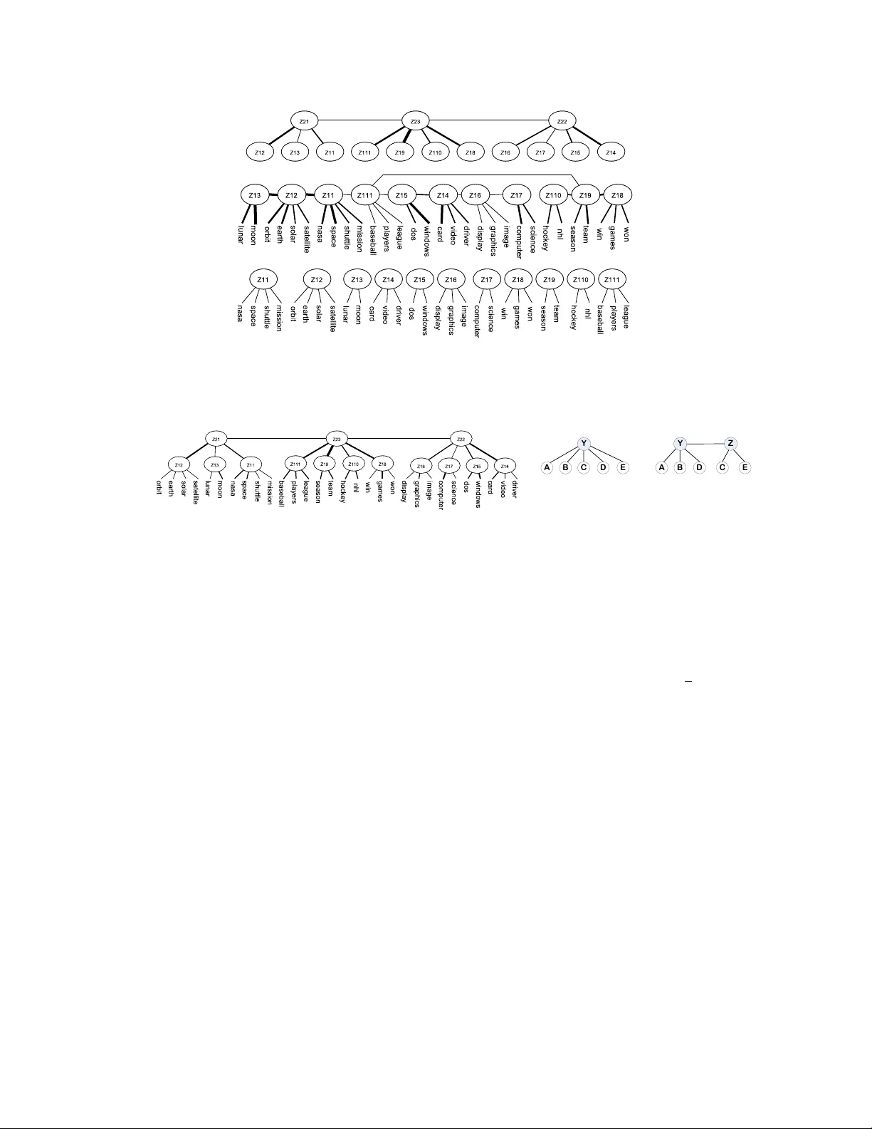
Pr ogr essiv e EM f or Latent T r ee Models and Hierar chical T opic Detection Peixian Chen ∗ Department of Computer Science The Hong K ong Uni versity of Science and T echnology pchenac@cse.ust.hk Nevin L. Zhang Department of Computer Science The Hong K ong Uni versity of Science and T echnology lzhang@cse.ust.hk Leonard K.M. Poon Department of Mathematics and Information T echnology The Hong K ong Institute of Education kmpoon@ied.edu.hk Zhourong Chen Department of Computer Science The Hong K ong Uni versity of Science and T echnology zchenbb@cse.ust.hk Abstract Hierar c hical latent tr ee analysis (HL T A) is recently proposed as a new method for topic detection. It dif fers fundamentally from the LD A-based methods in terms of topic definition, topic-document relationship, and learning method. It has been shown to discov er significantly more coherent topics and better topic hierarchies. Howe v er , HL T A relies on the Expectation-Maximization (EM) algorithm for pa- rameter estimation and hence is not ef ficient enough to deal with large datasets. In this paper, we propose a method to drastically speed up HL T A using a tech- nique inspired by recent adv ances in the moments method. Empirical e xperiments show that our method greatly impro ves the efficienc y of HL T A. It is as efficient as the state-of-the-art LD A-based method for hierarchical topic detection and finds substantially better topics and topic hierarchies. 1 INTR ODUCTION Detecting topics and topic hierarchies from document collections, along with its many potential ap- plications, is a major research area in Machine Learning. Currently the predominant approach to topic detection is latent Dirichlet allocation (LD A) (Blei et al., 2003). LD A has been developed to detect topics and to model relationships among them, including topic correlations (Blei and Laf ferty, 2007), topic hierarchies (Blei et al., 2010; Paisley et al., 2012), and topic ev olution (Blei and Laf- ferty, 2006). W e collectiv ely name these methods LD A-based methods . In those methods, a topic is a probability distribution over a vocabulary and a document is a mixture of topics. Therefore LDA is a type of mixtur e membership model . ∗ http://peixianc.me 1 A totally dif ferent approach to hierarchical topic detection is recently proposed by Liu et al. (2014). It is called hierar chical latent tr ee analysis (HL T A), where topics are organized hierarchically as a latent tr ee model (L TM) (Zhang, 2004; Zhang et al., 2008b) such as the one in Fig 1. In HL T A, a topic is a state of a latent variable and it corresponds to a collection of documents, and a document can belong to multiple topics. HL T A is therefore a type of multiple membership model . Empirical results from Liu et al. (2014) indicate that HL T A finds significantly better topics and topic hierarchies than hierar c hical latent Dirichlet allocation (hLD A), the first LDA-based method for hierarchical topic detection. Howe v er , HL T A does not scale up well. It took, for instance, 17 hours to process a NIPS dataset that consists of fe wer than 2,000 documents ov er 1,000 distinct words (Liu et al., 2014).(Note that hLD A took e ven longer time.) The computational bottleneck of HL T A lies in the use of the EM algorithm (Dempster et al., 1977) for parameter estimation. In this paper , we propose pr o gr essive EM (PEM) as a replacement of EM so as to scale up HL T A. PEM is motiv ated by the moments method, where parameters are determined by solving equations, each of which inv olv es a small number of model parameters related to two or three observed variables (Chang, 1996; Anandkumar et al., 2012). Similarly , PEM works in steps and, at each step, it focuses on a small part of the model parameters and in volv es only three or four observed v ariables. Our new algorithm is hence named PEM-HL T A. It is drastically faster than HL T A. PEM-HL T A finished processing the aforementioned NIPS dataset within 4 minutes. It only took around 11 hours, on a single desktop computer , to analyze a version of New Y ork T imes dataset that consists of 300,000 articles with 10,000 distinct w ords. PEM-HL T A is also as ef ficient as nHDP (Paisley et al., 2012), a state-of-the-art LD A-based method for hierarchical topic detection, and it significantly outperforms nHDP , as well as hLDA, in terms of the quality of topics and topic hierarchies. 2 PRELIMINARIES A latent tr ee model (L TM) is a Markov random field over an undirected tree, where the leaf nodes represent observed variables and the internal nodes represent latent variables (Zhang et al., 2008a). In this paper we assume all variables ha v e finite car dinality , i.e., finite number of possible states. Parameters of an L TM consist of potentials associated with edges and nodes such that the product of all potentials is a joint distribution ov er all variables. W e pick the potentials as follows: Root the model at an arbitrary latent node, direct the edges away from the root, and specify a marginal distribution for the root and a conditional distribution for each of the other nodes gi ven its parent. Then in Fig 2(b), if Y is the root, the parameters are the distributions P ( Y ) , P ( A | Y ) , P ( Z | Y ) , P ( C | Z ) and so forth. Because of the way the potentials are picked, L TMs are technically tree-structured Bayesian networks (Pearl, 1988). L TMs with a single latent variables are known as latent class models (LCMs) (Bartholomew and Knott, 1999). They are a type of finite mixture models for discrete data. For e xample, the model m 1 in Fig 2(a) defines the following mixture distrib ution o ver the observ ed variables: P ( A, · · · , E ) = X | Y | i =1 P ( Y = i ) P ( A, · · · , E | Y = i ) (1) where | Y | is the cardinality of Y . If the model is learned from a dataset, then the data are partitioned into | Y | soft clusters, each represented by a state of Y . The model m 2 in Fig 2(b) has two latent variables. Its joint distribution can be reduced to two dif ferent b ut related mixture distributions: P ( A, · · · , E ) = X | Y | i =1 P ( Y = i ) P ( A, · · · , E | Y = i ) , P ( A, · · · , E ) = X | Z | i =1 P ( Z = i ) P ( A, · · · , E | Z = i ) . 2 Figure 3: Intermediate models created by P E M - H LT A on a toy data set. The model giv es two different ways of partitioning the data, one represented by Y and the other by Z . Hence L TMs are a tool for multidimensional clustering (Chen et al., 2012). Figure 1: Latent tree model obtained from a toy text dataset. A Y B C D E (a) m 1 Y A B D E Z C (b) m 2 Figure 2: Leaf nodes are observed while others are latent. 3 THE ALGORITHM The input to our PEM-HL T A algorithm is a collection D of documents, each represented as a binary vector over a vocab ulary V . The values in the vector indicate the presence or absence of words in the document. The output is an L TM, such as the one shown in Fig 1, where the word variables are at the bottom and the latent variables, all assumed binary , form se veral levels of hierarchy on top. Each state of a latent variable corresponds to a cluster of documents and is interpreted as a topic. The top lev el control of PEM-HL T A is given in Algorithm 1, and subroutines in Algorithms 2 – 3. 3.1 TOP LEVEL CONTR OL W e illustrate the top level control using the example model in Fig 1, which is learned from a dataset with 30 word variables. In the first pass through the loop, the subroutine B U I L D I S L A N D S is called (line 3). It partitions all variables into 11 clusters (Fig 3 bottom), which are uni-dimensional in the sense that the co-occurrences of words in each cluster can be properly modeled using a single latent variable. A latent variable is introduced for each cluster to form an LCM. W e metaphorically refer to the LCMs as islands and the latent variables in them as le v el-1 latent v ariables. The next step is to link up the 11 islands (line 4). This is done by estimating the mutual information (MI) (Cover and Thomas, 2012) between every pair of latent v ariables and building a Cho w-Liu tree (Cho w and Liu, 1968) o ver them, so as to form an ov erall model (Liu et al., 2013). The result is the model at the middle of Fig 3. In the subroutine H A R D A S S I G N M E N T , inference is carried out to compute the posterior distrib ution of each latent v ariable for each document. The document is assigned to the state with the maximum posterior probability . This results in a dataset ov er the level-1 latent variables (line 10). In the second pass through the loop, the lev el-1 latent variables are partitioned into 3 groups and 3 islands are created. The islands are linked up to form the model shown at the top of Fig 3. At line 8, the model at the top of Fig 3 ( m 1 ) is stacked on the model in the middle ( m ) to giv e rise to the final model in Fig 1. While doing so, the subroutine S TAC K M O D E L S cuts off the links among the lev el-1 latent variables. The number of nodes at the top lev el is below the threshold τ , if we set τ = 5 , and hence the loop is e xited. EM is run on the final model for κ steps to improve its parameters (line 12). 3 Algorithm 1 P E M - H L TA( D , τ , δ , κ ) Inputs: D —Collection of documents, τ —Upper bound on the number of top-le vel topics, δ —Threshold used in UD-test, κ —Number of EM steps on final model. Outputs: An HL TM and a topic hierarchy . 1: D 1 ← D , L ← ∅ , m ← null . 2: repeat 3: L ← B U I L D I S L A N D S ( D 1 , δ ); 4: m 1 ← B R I D G E I S L A N D S ( L , D 1 ); 5: if m = null then 6: m ← m 1 ; 7: else 8: m ← S TAC K M O D E L S ( m 1 , m ); 9: end if 10: D 1 ← H A R D A S S I G N M E N T ( m , D ); 11: until |L| < τ . 12: Run EM on m for κ steps. 13: return m and topic hierarchy extracted from m . Algorithm 2 B U I L D I S L A N D S ( D , δ ) 1: V ← variables in D , M ← ∅ . 2: while |V | > 0 do 3: m ← O N E I S L A N D ( D , V , δ ); 4: M ← M ∪ { m } ; 5: V ← variables in D but not in any m ∈ M ; 6: end while 7: return M . In our experiments, we set κ = 50 . In Section 5.1 we will discuss how to extract a topic hierarchy from the final model. 3.2 BUILDING ISLANDS The pseudo code for the subroutine B U I L D I S L A N D S is given in Algorithm 2. It calls another sub- routine O N E I S L A N D to identify a uni-dimensional subset of observed variables and builds an LCM with them. Then it repeats the process on those observed variables left to create more islands, until all variables are included in these islands. Finally , it returns the set of all the islands. 3.2.1 UNI-DIMENSIONALITY TEST W e rely on the uni-dimensionality test (UD-test) (Liu et al., 2013) to determine whether a set S of variables is uni-dimensional. The idea is to compare two L TMs m 1 and m 2 , where m 1 is the best model among all LCMs for S while m 2 is the best model among all L TMs that contain two latent variables. The model selection criterion used is the BIC score (Schwarz, 1978). The set S is uni-dimensional if the following inequality holds: B I C ( m 2 | D ) − B I C ( m 1 | D ) < δ, (2) where δ is a threshold. In other words, S is considered uni-dimensional if the best two-latent vari- able model is not significantly better than the best one-latent variable model. The quantity on the left hand side of Equation (2) is a lar ge sample approximation of the natural logarithm of Bayes factor (Raftery, 1995) for comparing m 1 and m 2 . According to the cut-off values for the Bayes factor , we set δ = 3 in our e xperiments. 3.2.2 BUILDING AN ISLAND Giv en dataset D with variables V , the subroutine O N E I S L A N D identifies a uni-dimensional subset of variables and builds an LCM for them. Define the mutual information between a variable Z and a set S as MI ( Z, S ) = max A ∈S MI ( Z, A ) . O N E I S L A N D maintains a working set S of observed variables. Initially , S contains the pair of variables with the highest MI among all pairs, and a third variable that has the highest MI with the pair (line 2). At line 5, an LCM is learned for those three variables using the subroutine L E A R N L C M, which is given in the Appendix along with some other subroutines. Then other variables are added to S one by one until the UD-test fails. W e illustrate this process using Fig 2. Suppose S initially consists of three variables A , B , C . Let D be the variable that has the maximum MI with S among all other variables. Suppose the UD-test passes on S ∪ { D } , then D is added to S . Next let E be the variable with the maximum MI with S (line 7) and the UD-test is performed on S ∪ E = { A, B , C , D, E } (lines 8-14). The two models m 1 and m 2 used in the test is sho wn in Fig 2. For computational efficiency , we do not search for the best structure for m 2 . Instead, the structure is determined as follo ws: Pick the variable in S that has the maximum MI with E (line 8) (let it be C ), and group it with E in the model (line 12). The 4 Algorithm 3 O N E I S L A N D ( D , V , δ ) 1: if |V | ≤ 3 , m ← L E A R N L C M ( D , V ), return m . 2: S ← three variables in V with highest MI, 3: V 1 ← V \ S ; 4: D 1 ← P R O J E C T D AT A ( D , S ), 5: m ← L E A R N L C M ( D 1 , S ). 6: loop 7: X ← arg max A ∈V 1 M I ( A, S ) , 8: W ← arg max A ∈ S M I ( A, X ) , 9: D 1 ← P R O J E C T D AT A ( D , S ∪ { X } ) , V 1 ← V 1 \ { X } . 10: m 1 ← P E M - L C M ( m, S , X, D 1 ) . 11: if |V 1 | = 0 , return m 1 . 12: m 2 ← P E M - L T M - 2 L ( m , S \ { W } , { W , X } , D 1 ) 13: if B I C ( m 2 |D 1 ) − B I C ( m 1 |D 1 ) > δ then . 14: retur n m 2 with W , X and their parent re- mov ed. 15: end if 16: m ← m 1 , S ← S ∪ { X } . 17: end loop model parameters are estimated using the subroutines P E M - L C M and P E M - L T M - 2 L, which will be explained in the next section. If the test fails, then C , E and Z are removed from m 2 , and what remains in the model, an LCM, is returned. If the test passes, E is added to S (line 16) and the process continues. 4 PR OGRESSIVE EM FOR MODEL CONSTRUCTION PEM-HL T A conceptually consists of a model construction phase (lines 2-11) and a parameter esti- mation phase (line 12). During the first phase, many intermediate models are constructed. In this section, we present a fast method for estimating the parameters of those intermediate models. 4.1 MOMENTS METHOD FOR P ARAMETER ESTIMA TION W e begin by presenting a property of L TMs that motiv ates our new method. A similar property of HMMs was first discovered by Chang (1996). W e introduce some notations using m 1 of Fig 2. Since all variables have the same cardinality , the conditional distribution P ( A | Y ) can be regarded as a square matrix, which we denote as P A | Y . Similarly , P AC is the matrix representation of the joint distribution P ( A, C ) . For a v alue b of B , P b | Y is the vector presentation of P ( B = b | Y ) and P AbC the matrix representation of P ( A, B = b, C ) . Theorem 1 [ Zhang et al. (2014)] Let Y be the latent variable in an LCM and A, B , C be thr ee of the observed variables. Assume all variables have the same cardinality and the matrices P A | Y and P AC ar e in vertible . Then we have P A | Y diag( P b | Y ) P − 1 A | Y = P AbC P − 1 AC , (3) wher e diag( P b | Y ) is a diagonal matrix with components of P b | Y as the diagonal elements. The equation implies that the model parameters P ( B = b | Y =0) , · · · , P ( B = b | Y = | Y | ) are the eigen- values of the matrix on the right, and hence can be obtained from the marginal distributions P AbC P AC . Theorem 1 can be used to estimate P ( B | Y ) under two conditions: (1) There is a good fit between the data and model as if the data were generated from the model, and (2) the sample size is sufficiently large. In this case, the empirical marginal distributions ˆ P ( A, B , C ) and ˆ P ( A, C ) computed from data are accurate estimates of the distributions P ( A, B , C ) and P ( A, C ) of the model. W e can use them to form the matrix P AbC P − 1 AC , and determine P B | Y as the eigenv alues of the matrix. This is called the moments method. Note that Theorem 1 still applies when replacing edges like ( Y , A ) with paths. For example in Fig 2(b), if P ( C | Z ) and P ( E | Z ) are to be estimated, a third observed variable can be chosen from ( A, B , D ) as long as there is path from Z to this observed v ariable. Theorem 1 can be also used to estimate all the parameters of the model m 1 in Fig 2. First, we can estimate P ( B | Y ) using Equation 3 in the sub-model Y - { A, B , C } . By swapping the roles of variables, we can also estimate P ( A | Y ) and P ( C | Y ) in the sub-model. Next we can consider the sub-model Y - { B , C, D } and estimate P ( D | Y ) with P ( B | Y ) and P ( C | Y ) fixed. Finally , we can consider the sub-model Y - { C, D , E } and estimate P ( E | Y ) there with P ( C | Y ) and P ( D | Y ) fixed. Note that the parameters are estimated in steps instead of all at once. Hence we call this scheme pr ogr essive parameter estimation . 5 4.2 PROGRESSIVE EM The moments method is not iterativ e and hence can be drastically faster than EM. Unfortunately , it does not produce high quality estimates when the model does not fit data well and/or the sample size is not sufficiently large. In such cases, the empirical marginal distributions ˆ P ( A, B , C ) and ˆ P ( A, C ) are poor estimates of the distributions P ( A, B , C ) and P ( A, C ) of the model. In our experiences, the method frequently gi ves negati v e estimates for probability values in the context of latent tree models. In this paper , we do not estimate parameters by solving the equation in Theorem 1. Howe v er , we adopt the progressiv e estimation scheme and combine it with EM. This gives rise to pro gr ess EM (PEM) . T o estimate the parameters of m 1 , PEM first estimates P ( Y ) , P ( A | Y ) , P ( B | Y ) , and P ( C | Y ) by running EM on the sub-model Y - { A, B , C } ; then it estimates P ( D | Y ) by running EM on the sub-model Y - { B , C , D } with P ( B | Y ) , P ( C | Y ) and P ( Y ) fixed; and finally it estimates P ( E | Y ) on sub-model Y - { C , D, E } similarly . All the sub-models in v olve 3 observ ed v ariables. For m 2 , PEM first estimates P ( Y ) , P ( A | Y ) , P ( B | Y ) and P ( D | Y ) by running EM on sub-model Y - { A, B , D } ; then it estimates P ( C | Z ) , P ( E | Z ) and P ( Z | Y ) by running EM on the two latent variable sub-model { B , D } - Y - Z - { C, E } , with P ( B | Y ) , P ( D | Y ) and P ( Y ) fixed. Note that only two of the children of Y are used here, and the model in v olves only 4 observ ed variables. Intuitiv ely , the moments method tries to fit data in a rigid way , while PEM tries to fit data in an elastic manner . It nev er giv es negati ve probability values. Moreover , it is still efficient because EM is run only on sub-models with three or four observed binary v ariables, and local maxima is seldom an issue using multiple starting points. 4.3 PEM FOR ISLAND BUILDING PEM can be aligned with the subroutine O N E I S L A N D nicely because the subroutine adds variables to the working set S one at a time. Consider a pass through the loop. At the beginning, we have an LCM m for the variables in S , whose parameters hav e been estimated earlier . Then O N E I S L A N D finds the variable X outside S that has the maximum MI with S , and the variable W inside S that has the maximum MI with X (line 7, 8). At line 11, O N E I S L A N D adds X to the m to create a new LCM m 1 , and estimates the parameters for the ne w variable using the subroutine P E M - L C M . W e illustrate how this is done using Fig 2. Suppose the LCM m is the model Y - { A, B , C, D } and the variable X is E . P E M - L C M adds the variable E to m and thereby creates a new LCM m 1 , which is Y - { A, B , C, D , E } (Fig 2 left). T o estimate the distribution P ( E | Y ) , P E M - L C M creates a temporary model m 0 from m 1 by only keeping three observed variables: E and two other variables with maximum MI with E . Suppose m 0 is Y - { C , D , E } . P E M - L C M estimates the distribution P ( E | Y ) by running EM on m 0 with all other parameters fixed. Finally , it copies P ( E | Y ) from m 0 to m 1 , and returns m 1 . At line 12, O N E I S L A N D adds X to m and learns a two-latent variable model m 2 using the subroutine P E M - L T M - 2 L . W e illustrate P E M - L T M - 2 L using the foregoing example. Let X be E and W be C . P E M - L T M - 2 L creates the new model m 2 , which is { A, B , D } - Y - Z - { C, E } (Fig 2 right). T o estimate the parameters P ( C | Z ) , P ( E | Z ) and P ( Z | Y ) , P E M - L T M - 2 L creates a temporary model m 0 which is { A, D } - Y - Z - { C , E } . Only the two of the children of Y that ha ve maximum MI with E remain( A and D in this example). P E M - L T M - 2 L estimates the three distributions by running EM on m 0 with all other parameters fixed. Finally , it copies the distributions from m 0 to m 2 and returns m 2 . 1 Similarly in the subroutine B R I D G E D I S L A N D S we use this method to estimate parameters for edges between latent v ariables, b ut only estimating P ( Z | Y ) and keeping all other parameters fixed. 5 EMPIRICAL RESUL TS W e aim at scaling up HL T A, hence we need to empirically determine how efficient PEM-HL T A is compared with HL T A. W e also compare PEM-HL T A with nHDP , the state-of-the-art LDA-based method for hierarchical topic detection, in terms of computational efficienc y and quality of results. Also included in the comparisons are hLDA and a method named CorEx (V er Steeg and Galstyan, 2014) that b uilds hierarchical latent trees by optimizing an information-theoretic objecti ve function. 1 Details of P E M - L C M and P E M - LTM - 2 L can be found in the Appendix submitted as a supplement. 6 T wo of the datasets used are NIPS data 2 and Newsgroup 3 . Three versions of the NIPS data with vocab ulary sizes 1,000, 5,000 and 10,000 were created by choosing words with highest average TF-IDF values, referred to as Nips-1k, Nips-5k and Nips-10k. Similarly , two versions (News-1k and News-5k) of the Newsgroup data were created. Note that Ne ws-10k is not included because it is beyond the capabilities of three of the methods. Comparisons of PEM-HL T A and nHDP on large-scale data will be giv en separately in Section 5.4. After preprocessing, NIPS and Newsgroup consist of 1,955 and 19,940 documents respecti v ely . For PEM-HL T A, HL T A and CorEx, the data are represented as binary vectors, whereas for nHDP and hLD A, the y are represented as bags-of-words. PEM-HL T A determines the height of hierarchy and the number of nodes at each level automatically . On the NIPS and Newsgroup datasets, it produced hierarchies with between 4 to 6 le vels. For nHDP and hLD A, the height of hierarchy needs to be manually set and is usually set at 3. W e set the number of nodes at each lev el in such way that nHDP and hLD A would yield roughly the same total number of topics as PEM-HL T A. CorEx were configured similarly . PEM-HL T A is implemented in Jav a. The parameter settings are described in Section 3. Implementations of other algorithms were provided by their authors and ran at their default parameter settings. All experiments are conducted on the same desktop computer . 5.1 TOPIC HIERARCHIES FOR NIPS-10K T able 1 shows parts of the topic hierarchies obtained by nHDP and PEM-HL T A. The left half dis- plays 3 top-lev el topics by nHDP and their children. Each nHDP topic is represented using the top 5 words occurring with highest probabilities in the topic. The right half show 3 top-lev el topics yielded by PEM-HL T A and their children. The topics are extracted from the model learned by PEM-HL T A as follo ws: For a latent binary variable Z in the model, we enumerate the w ord v ariables in the sub- tree rooted at Z in descending order of their MI values with Z. The leading words are those whose probabilities differ the most between the two states of Z and are hence used to characterize the states. The state of Z under which the words occur less often overall is regarded as the backgr ound topic and is not reported, while the other state is reported as a genuine topic. V alues in [] show the percentage of the documents belonging to the genuine topic. Let us e xamine some of the topics. W e refer to topics on the left using the letter L follo wed by topic numbers and those on the right using R. For PEM-HL T A, R1 consists of probability terms: R1.1 is about EM algorithm; R1.2 about Gaussian mixtures and R1.3 about generative distributions. R1.4 is a combination of variance and noise, which are separated at the next lower lev el. For nHDP , the topic L1 and its children L1.1, L1.2 and L1.5 are also about probability . Howe ver , L1.3 and L1.4 do not fit in the group well. The topic R2 is about image analysis, while its first four subtopics are about different aspects of image analysis: sour ces of images, pixels, objects . R2.5 and R2.6 are also meaningful and related, but do not fit in well. They are placed in another subgroup by PEM- HL T A. In nHDP , the subtopics of L2 do not giv e a clear spectrum of aspects of image analysis. The topic R3 is about speech recognition. Its subtopics are about dif ferent aspects of speech recognition. Only R3.4 does not fit in the group well. In contrast, L3 and its subtopics do not present a clear semantic hierarchy . Some of them are not meaningful. Another topic related to speech recognition L1.5 is placed elsewhere. Overall, the topics and topic hierarchy obtained by PEM-HL T A are more meaningful than those by nHDP . 5.2 TOPIC COHERENCE AND MODEL QU ALITY T o quantitatively measure the quality of the topics, we use the topic coher ence scor e proposed by Mimno et al. (2011). The metric depends on the number M of words used to characterize a topic. W e set M = 4 . In addition, we use held-out likelihood to assess the quality of the models produced by the fiv e algorithms. Each dataset was randomly partitioned into a training set with 80% of the data, and a test set with 20% of the data. T able 2 shows the av erage topic coherence scores of the topics produced by the five algorithms. The sign “-” indicates running time exceeded 72 hours. The quality of topics produced by PEM-HL T A is similar to those by HL T A on Nips-1k and News-1k, and better on Nips-5k. In all cases, PEM- HL T A produced significantly better topics than nHDP and the other two algorithms. The held-out per-document loglikelihood statistics are shown in T able 3. The likelihood values of PEM-HL T A 2 http://www .cs.nyu.edu/ roweis/data.html 3 http://qwone.com/jason/20Ne wsgroups/ 7 T able 1: Parts of the topic hierarchies obtained by nHDP (left) and PEM-HL T A (right) on Nips-10k. 1. gaussian likelihood mixture density Bayesian 1.1. gaussian density likelihood Bayesian 1.2. frey hidden posterior chaining log 1.3. classifier classifiers confidence 1.4. smola adaboost onoda mika svms 1.5. speech context hme hmm experts 2. image recognition images feature featur es 2.1. image recognition feature images object 2.2. smola adaboost onoda utterance 2.3. object matching shape image features 2.4. nearest basis examples rbf classifier 2.5. tangent distance simard distances 3. rules language rule sequence context 3.1. recognition speech mlp word trained 3.2. rules rule stack machine examples 3.3. voicing syllable fault faults units 3.4. rules hint table hidden structure 3.5. syllable stress nucleus heavy bit 1. [0.22] mixture gaussian mixtures em co variance 1.1. [0.23] em maximization ghahramani expectation 1.2. [0.23] mixture gaussian mixtures covariance 1.3. [0.23] generative dis generafive generarive 1.4. [0.27] variance noise exp variances deviation 1.4.1. [0.28] variance exp variances deviation cr 1.4.2. [0.44] noise noisy robust robustness mea 2. [0.26] images image pixel pixels object 2.1. [0.25] images image features detection face 2.2. [0.24] camera video imaging false tracked 2.3. [0.24] pixel pixels intensity intensities 2.4. [0.17] object objects shape views plane 2.5. [0.20] rotation invariant translation 2.6. [0.26] nearest neighbor kohonen neighbors 3. [0.15] speech word speaker language phoneme 3.1. [0.16] word language vocabulary words sequence 3.2. [0.11] spoken acoustics utterances speakers 3.3. [0.10] string strings grammar symbol symbols 3.4. [0.06] retrieval search semantic searching 3.5. [0.14] phoneme phonetic phonemes waibel lang 3.6. [0.15] speech speaker acoustic hmm hmms are similar to those of HL T A, sho wing that the use of PEM to replace EM does not influence model quality much. They are significantly higher than those of CorEx. Note that the likelihood values in T able 3 for the LD A-based methods are calculated from bag-of-w ords data. They are still lower than the other methods ev en calculated from the same binary data as for the other three methods. It should be noted that, in general, better model fit does not necessarily imply better topic quality (Chang et al., 2009). In context of hierarchical topic detection, howe ver , PEM-HL T A not only leads to better model fit, b ut also gi ves better topics and better topic hierarchies. T able 2: A verage topic coherence scores. Nips-1k Nips-5k Nips-10k News-1k News-5k PEM-HL T A -6.25 -8.04 -8.87 -12.30 -13.07 HL T A -6.23 -9.23 — -12.08 — hLD A -6.99 -8.94 — — — nHDP -8.08 -9.55 -9.86 -14.26 -14.51 CorEx -7.23 -9.85 -10.64 -13.47 -14.51 T able 3: Per-document loglikelihood Nips-1k Nips-5k Nips-10k News-1k News-5k PEM-HL T A -390 -1,117 -1,424 -116 -262 HL T A -391 -1,161 — -120 — hLD A -1,520 -2,854 — — — nHDP -3,196 -6,993 -8,262 -265 -599 CorEx -442 -1,226 -1,549 -140 -322 5.3 RUNNING TIMES T able 4 sho ws the running time statistics. PEM-HL T A drastically outperforms HL T A, and the dif fer- ence increases with vocab ulary size. On Nips-10k and News-5k, HL T A did not terminate in 3 days, while PEM-HL T A finished the computation in about 6 hours. PEM-HL T A is also faster than nHDP , although the difference decreases with vocab ulary size as nHDP works in a stochastic way (Paisley et al., 2012). Moreover , PEM-HL T A is more ef ficient than hLDA and CorEx. T able 4: Running times. T ime(min) Nips-1k Nips-5k Nips-10k News-1k News-5k PEM-HL T A 4 140 340 47 365 HL T A 42 2,020 — 279 — hLD A 2,454 4,039 — — — nHDP 359 382 435 403 477 CorEx 43 366 704 722 4,025 T able 5: Performances on the New Y ork Times data. T ime (min) A verage topic coherence PEM-HL T A 670 -12.86 hHDP 637 -13.35 5.4 STOCHASTIC EM Conceptually , PEM-HL T A has two phases: hierarchical model construction and parameter estima- tion. In the second phase, EM is run a predefined number of steps from the initial parameter values from the first phase. It is time-consuming if the sample size is large. Paisley et al. (2012) faced a similar problem with nHDP . They solve the problem using stochastic inference. The idea is to divide the data set into subsets and process the subsets one by one. Model parameters are updated after processing each data subset and o verall one goes through the entire data set only once.W e adopt the same idea for the second phase of PEM-HL T A and call it stochastic EM . W e tested the idea on the 8 New Y ork Times dataset 1 , which consists of 300,000 articles. T o analyze the data, we pick ed 10,000 words using TF-IDF and then randomly divided the dataset into 50 equal-sized subsets. W e used only the fist subset for the first phase of PEM-HL T A. For the second phase, we ran EM on current model once using each subset in turn until all the subsets are utilized . On New Y ork Times data, we only compare PEM-HL T A with nHDP since other methods are not amenable to processing lar ge datasets as we can observe from T able 4. W e still trained nHDP model using documents in bag-of-words form and PEM-HL T A using documents as binary vectors of words. T able 5 reports the running times and topic coherence. PEM-HL T A took around 11 hours which is a little bit slower than nHDP (10.5 hours). Howe ver , PEM-HL T A produced more coherent topics, which is not only testified by the coherence score, b ut also the resulting topic hierarchies. The reader could get a clear picture of the superiority of PEM-HL T A over nHDP by taking a quick look at the model structure and topic hierarchies submitted as supplements. 6 CONCLUSIONS W e have proposed and in vestigated a method to scale up HL T A — a newly emerged method for hierarchical topic detection. The key idea is to replace EM using progressive EM. The resulting algorithm PEM-HL T A reduces the computation time of HL T A drastically and can handle much larger datasets. More importantly , it outperforms nHDP , the state-of-the-art LDA-based method for hierarchical topic detection, in terms of both quality of topics and topic hierarchy , with comparable speed on large-scale data. Although we only sho w ho w PEM works in HL T A, PEM can possibly be used in other more general models. PEM-HL T A can also be further scaled up through parallelization and used for text classification. W e plan to in vestigate these directions in the future. 1 http://archiv e.ics.uci.edu/ml/datasets/Bag+of+W ords 9 References Animashree Anandkumar, Kamalika Chaudhuri, Daniel Hsu, Sham M. Kakade, Le Song, and T ong Zhang. Spectral methods for learning multivariate latent tree structure. In Advances in Neural Information Process- ing Systems , pages 2025–2033, 2012. David J. Bartholomew and Martin Knott. Latent V ariable Models and F actor Analysis . Arnold, 2nd edition, 1999. David M Blei and John D Lafferty . Dynamic topic models. In Pr oceedings of the 23r d international confer ence on Machine learning , pages 113–120. A CM, 2006. David M Blei and John D Lafferty . A correlated topic model of science. The Annals of Applied Statistics , pages 17–35, 2007. David M. Blei, Andre w Y . Ng, and Michael I. Jordan. Latent Dirichlet allocation. Journal of Machine Learning Resear ch , 3:993–1022, 2003. David M. Blei, Thomas L. Grif fiths, and Michael I. Jordan. The nested Chinese restaurant process and Bayesian nonparametric inference of topic hierarchies. J ournal of the ACM , 57(2):7:1–7:30, 2010. Jonathan Chang, Jordan L Boyd-Graber , Sean Gerrish, Chong W ang, and David M Blei. Reading tea leav es: How humans interpret topic models. In Advances in Neural Information Pr ocessing Systems , volume 22, pages 288–296, 2009. Joseph T . Chang. Full reconstruction of Markov models on evolutionary trees: Identifiability and consistency . Mathematical Biosciences , 137(1):51–73, 1996. T ao Chen, Nevin L. Zhang, T engfei Liu, Kin Man Poon, and Y i W ang. Model-based multidimensional cluster- ing of categorical data. Artificial Intelligence , 176:2246–2269, 2012. C. K. Chow and C. N. Liu. Approximating discrete probability distributions with dependence trees. IEEE T ransactions on Information Theory , 14(3):462–467, 1968. Thomas M Cov er and Joy A Thomas. Elements of information theory . John Wile y & Sons, 2012. Arthur P . Dempster , Nan M. Laird, and Donald B. Rubin. Maximum likelihood from incomplete data via the EM algorithm. J ournal of the Royal Statistical Society . Series B (Methodological) , 39(1):1–38, 1977. T eng-Fei Liu, Nevin L. Zhang, Peixian Chen, April Hua Liu, Leonard K.M. Poon, and Y i W ang. Greedy learning of latent tree models for multidimensional clustering. Machine Learning , 98(1–2):301–330, 2013. T engfei Liu, Ne vin L. Zhang, and Peixian Chen. Hierarchical latent tree analysis for topic detection. In Machine Learning and Knowledge Discovery in Databases , pages 256–272, 2014. David Mimno, Hanna M W allach, Edmund T alley , Miriam Leenders, and Andrew McCallum. Optimizing semantic coherence in topic models. In Proceedings of the Confer ence on Empirical Methods in Natural Language Pr ocessing , pages 262–272. Association for Computational Linguistics, 2011. John P aisley , Chong W ang, Da vid M Blei, and Michael I Jordan. Nested hierarchical dirichlet processes. IEEE T ransactions on P attern Analysis and Machine Intelligence , 37, 2012. Judea Pearl. Pr obabilistic Reasoning in Intelligent Systems: Networks of Plausible Inference . Morg an Kauf- mann Publishers, San Mateo, California, 1988. Adrian E. Raftery . Bayesian model selection in social research. Sociological Methodology , 25:111–163, 1995. Gideon Schwarz. Estimating the dimension of a model. The Annals of Statistics , 6(2):461–464, 1978. Greg V er Steeg and Aram Galstyan. Discovering structure in high-dimensional data through correlation e xpla- nation. In Advances in Neural Information Pr ocessing Systems 27 , pages 577–585, 2014. Nevin L. Zhang. Hierarchical latent class models for cluster analysis. Journal of Machine Learning Resear ch , 5:697–723, 2004. Nevin L. Zhang, Y i W ang, and T ao Chen. Latent tree models and multidimensional clustering of categorical data. T echnical Report HKUST -CS08-02, The Hong Kong Uni veristy of Science and T echnology , 2008a. Nevin L. Zhang, Y i W ang, and T ao Chen. Discovery of latent structures: Experience with the CoIL challenge 2000 data set. J ournal of Systems Science and Complexity , 21:172–183, 2008b. Nevin L. Zhang, Xiaofei W ang, and Peixian Chen. A study of recently discovered equalities about latent tree models using in verse edges. In Pr obabilistic Graphical Models , pages 567–580, 2014. 10