Adaptivity and Computation-Statistics Tradeoffs for Kernel and Distance based High Dimensional Two Sample Testing

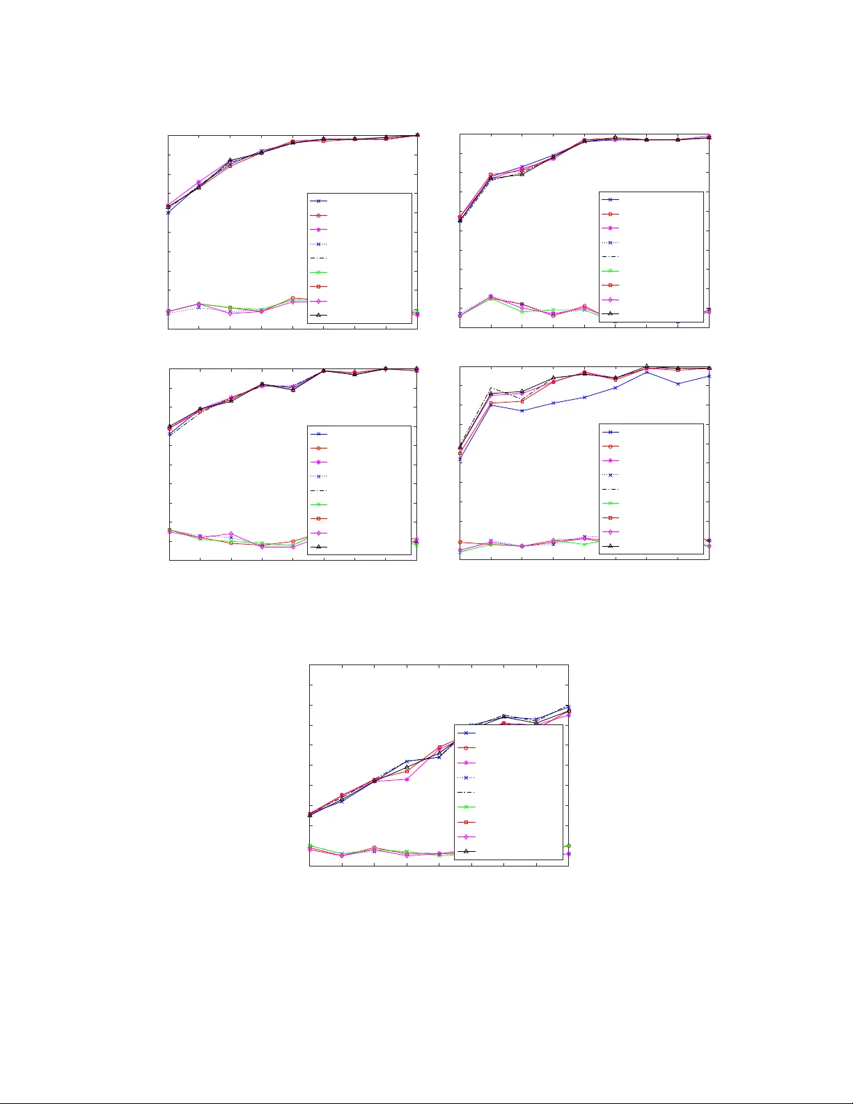
Adapti vity and Computation-Statistics T radeof fs for K ernel and Distance based High Dimensional T wo Sample T esting Aaditya Ramdas 12 aramdas@cs.cmu.edu Sashank J. Reddi 2 sjakkamr@cs.cmu.edu Barnab ´ as P ´ oczos 2 bapoczos@cs.cmu.edu Aarti Singh 2 aarti@cs.cmu.edu Larry W asserman 12 larry@stat.cmu.edu Department of Statistics 1 and Machine Learning Department 2 Carnegie Mellon Uni versity August 5, 2015 Abstract Nonparametric two sample testing is a decision theoretic problem that in volves identifying differences between two random v ariables without making parametric assumptions about their underlying distributions. W e refer to the most common settings as mean difference alternatives (MD A), for testing differences only in ﬁrst moments, and general difference alternati ves (GD A), which is about testing for an y dif ference in dis- tributions. A large number of test statistics hav e been proposed for both these settings. This paper connects three classes of statistics - high dimensional variants of Hotelling’ s t-test, statistics based on Reproducing Kernel Hilbert Spaces, and energy statistics based on pairwise distances. W e ask the following question - how much statistical power do popular kernel and distance based tests for GD A have when the unknown distributions dif fer in their means, compared to specialized tests for MD A? T o answer this, we formally characterize the power of popular tests for GD A like the Maximum Mean Discrepancy with the Gaussian k ernel ( gMMD ) and bandwidth-dependent variants of the Energy Distance with the Euclidean norm ( eED ) in the high-dimensional MD A regime. W e prove sev eral interesting prop- erties relating these classes of tests under MD A, which include (a) eED and gMMD hav e asymptotically equal power; furthermore the y also enjoy a free lunch be- cause, while they are additionally consistent for GD A, they hav e the same power as specialized high-dimensional t-tests for MDA. All these tests are asymptotically optimal (including matching constants) for MD A under spherical cov ariances, according to simple lower bounds. (b) The power of gMMD is independent of the kernel bandwidth, as long as it is larger than the choice made by the median heuristic. (c) There is a clear and smooth computation-statistics tradeoff for linear-time, subquadratic-time and quadratic-time versions of these tests, with more computation resulting in higher po wer . 1 All three observations are practically important, since point (a) implies that eED and gMMD while being consistent against all alternatives, are also automatically adapti ve to simpler alternativ es, point (b) suggests that the median “heuristic” has some theoretical justiﬁcation for being a default bandwidth choice, and point (c) implies that expending more computation may yield direct statistical beneﬁt by orders of magnitude. 1 Intr oduction Nonparametric two sample testing (or homogeneity testing) deals with detecting differences between two distributions, given samples from both, without making any parametric distributional assumptions. More formally , given samples X 1 , ..., X n ∼ P and Y 1 , ..., Y m ∼ Q , where P and Q are distributions in R d , the most common types of two sample tests in v olve testing for the follo wing sets of null and alternate hypotheses General difference alternati ves (GD A) : H 0 : P = Q vs H 1 : P 6 = Q, Mean difference alternati ves (MD A) : H 0 : µ P = µ Q vs H 1 : µ P 6 = µ Q where µ P := E P X, µ Q := E Q Y . This problem has a sustained interest in both the statistics and machine learning literature, due to applications where the sample size might be limited compared to dimensionality , due to experimental or computational costs. For example, it can be used to answer questions in medicine ( is there a differ ence between pill and placebo? ) and neuroscience ( does a particular brain r e gion respond differ ently to two dif ferent kinds of stimuli? ). W e will assume m = n for simplicity , though our results may be extended to the case when m/ ( n + m ) con ver ges to any constant k ∈ (0 , 1) . A test η is a function from X 1 , ...X n , Y 1 , ..., Y n to { 0 , 1 } , where we reject H 0 when η = 1 . W e will only consider tests that have an asymptotic type-I error of at most α . Let us call the set of all such tests as [ η ] n,d,α := { η : R n × d × R n × d → { 0 , 1 } , E H 0 η ≤ α + o (1) } . (1) In the Neyman-Pearson paradigm for the ﬁxed d setting, a test is judged by its power φ = φ ( n, P , Q, α ) = E H 1 η , and we say that such a test η ∈ [ η ] n,d,α is consistent in the ﬁxed d setting when E H 1 η → 1 , E H 0 η ≤ α as n → ∞ for any ﬁxed α > 0 . In contrast, we say that a test η ∈ [ η ] n,d,α is consistent in the high-dimensional setting when its power φ = φ ( n, d n , P n , Q n , α ) = E H 1 η satisﬁes E H 1 η → 1 , E H 0 ≤ α as ( n, d ) → ∞ , for any ﬁxed α > 0 where one also needs to specify the relati ve rate at which n, d can increase. The central question being considered in this paper is “what is the power of tests designed for GD A, compared to those designed for MD A, when the distrib utions truly differ in their means?” . W e will e xplain this and other related questions in more detail in Section 3. Remark 1. The tests consider ed in this paper have some common properties. All the test statistics T ar e center ed under the null, i.e . E H 0 T = 0 , dividing the statistic by p v ar ( T ) leads to an asymptotically standar d normal statistic under the null, i.e. T / p v ar ( T ) N (0 , 1) under H 0 , wher e repr esents conver g ence in distribution as n → ∞ , and hence all tests ar e of the form: η ( X 1 , ..., X n , Y 1 , ..., Y n ) = I T p v ar ( T ) > z α ! wher e z α is the 1 − α quantile of the standar d normal distribution. 2 T wo-sample testing is a fundamental decision-theoretic problem, having a long history in statistics - for example, the past century has seen a wide adoption of the t-statistic by Hotelling [1931] to decide if two samples ha ve dif ferent population means (MD A). It was introduced in the parametric setting for uni variate Gaussians, but it has been generalized to multiv ariate non-Gaussian settings as well. If ¯ X , ¯ Y are the sample means, and S is a joint sample cov ariance matrix, then a statistician using the multi variate t -test calculates T H := ( ¯ X − ¯ Y ) T S − 1 ( ¯ X − ¯ Y ) and the test is I ( T H / p V ar ( T H ) > t α ) where t α is chosen so that E H 0 η ≤ α + o (1) ). T H is consistent for MD A whenever P, Q hav e different means, and further , it is known to be the “uniformly most powerful” test when P , Q are uni variate Gaussians under fairly general assumptions [Kariya, 1981, Simaika, 1941, Anderson, 1958, Salaevskii, 1971]. In a seminal paper by Bai and Saranadasa [1996], the authors proved that T H has asymptotic po wer tending to α in this high-dimensional setting (as discussed in the next section), moti vating the study of alternativ e test statistics. Despite their increasing popularity and usage, many interesting questions remain unanswered, as will be discussed in Section 3 and partially answered in this paper . This paper deals with (moderately) high-dimensional and nonparametric two-sample testing, where d can grow polynomially with n , and there are no explicit parametric assumptions on P, Q . In Section 7, we experimentally validate our claims for a v ariety of distributions, ev en at quite small sample sizes and dimensions. This shows that the asymptotics accurately describe ev en ﬁnite sample behavior of these tests. Paper Outline. The rest of this paper is organized as follows. In Section 2, we introduce three classes of tests in the literature - Hotelling-based tests for MD A, and kernel-based and distance-based tests for GD A, and we discuss related open questions in Section 3. In Section 4, we prove that three of the most popular tests (one from each class) hav e the same asymptotic power for MD A, sho wing the free adaptivity of GD A-based tests for the simpler MD A problem. In Section 5, we sho w that all these classes of tests are optimal for MD A under the diagonal covariance setting, by adapting a lower bound from the normal means problem. Section 6 discusses computation-statistics tradeoffs, where we compare the power of linear-time, sub-quadratic time and quadratic-time versions of these tests. In Section 7, we run experiments and discuss some practical implications of this work. W e end with the proofs in Section 8. Notation W e use the standard o, o P , O P notation extensi vely . Also, for two non-random sequences A n , B n , A n = Ω( B n ) is the negation of A n = o ( B n ) , A n = ω ( B n ) is the negation of A n = O ( B n ) , and A n  B n to mean A n = B n ( c + o (1)) for some absolute constant c . T r () is the trace of a (square) matrix and T r k () is the k -th power of the trace. ◦ is the elementwise or Hadamard product, T s () refers to the total sum of all the elements of a matrix, e i is the i -th standard basis vector , 1 is the vector of ones. is con vergence in distribution, and I ( · ) is a 0-1 indicator function. 2 Hotelling-based MD A T ests and Ker nel/Distance-based GD A tests T ests for MD A . As mentioned in the introduction, Bai and Saranadasa [1996] prove that Hotelling’ s T H has power tending to α (this is called trivial po wer), when ( n, d ) → ∞ with d/n → 1 −  for small  , explained by the inherent difﬁculty of accurately estimating the O ( d 2 ) parameters of Σ − 1 with very fe w samples ( S − 1 is not ev en deﬁned if d > n and is badly conditioned if d is of similar order as n ). T o av oid this problem, they proposed to use the test statistic T B S := k ¯ X − ¯ Y k 2 − tr( S ) /n and showed that it has non-trivial power whenev er d/n → c ∈ (0 , ∞ ) . An important precursor to this non- parametric work of Bai and Saranadasa [1996] is that of Dempster [1958] who proposed a high-dimensional t-test for Gaussians. Sriv astav a and Du [2008] and Sri vasta va et al. [2013] proposed to instead use diag( S ) − 1 3 instead of S − 1 , in T H , and sho wed its adv antages in certain settings over T B S (speciﬁcally its scale in v ari- ance, i.e. inv ariance when the data is rescaled by a diagonal matrix, gi ves it an advantage when the cov ariance matrices are diagonal but non-spherical). In another extension of T B S by Chen and Qin [2010], henceforth called CQ, the authors proposed a variant of T B S of the form T C Q := 1 n ( n − 1) n X i 6 = j =1 X T i X j + 1 n ( n − 1) n X i 6 = j =1 Y T i Y j − 2 n 2 n X i,j =1 X T i Y j , analyzing its power for MDA when the cov ariances of X , Y are also unequal and without explicit restrictions on d, n , but rather in terms of conditions stated in terms of n, Σ and mean difference δ := µ P − µ Q . W e will return to these conditions later in this paper , since we will use assumptions of similar ﬂav or . Note that E [ T C Q ] = µ T P µ P + µ T Q µ Q − 2 µ T P µ Q = k µ P − µ Q k 2 , and hence T C Q is an unbiased estimator of k µ P − µ Q k 2 . In this paper , instead of using T C Q directly , we will analyze a minor variant, which is a U-statistic: U C Q := 1 n ( n − 1) n X i 6 = j =1 h C Q ( X i , X j , Y i , Y j ) where h C Q ( X, X 0 , Y , Y 0 ) := X T X + Y T Y − X T Y 0 − X 0 T Y . (2) T C Q ’ s dif ference from U C Q is only in the third term, and this dif ference is asymptotically v anishing, making the asymptotic properties of U C Q (especially its power) identical to T C Q , and its usage is only for technical con venience. There is also a lar ge literature on the so-called parametric Behrens-Fisher problem, which is a parametric MD A problem where the distributions are Gaussian and heteroskedastic, and also the nonparametric Behrens- Fisher problem that deals with MD A when P, Q are nonparametric mean-scale families, in the univ ariate and multiv ariate settings. See Belloni and Didier [2008] and Lopes et al. [2011] for recent such works, and references therein. Another related line of work analyzes the setting where p could be exponentially larger than n but assuming some kind of sparsity (say in the mean difference); see Cai et al. [2014] for such an example. T ests for GDA . It is well known that the K olmogorov-Smirnov (KS) test by Kolmogoro v [1933] and Smirnov [1948] in v olves dif ferences in empirical CDFs. The KS test, the related Cramer v on-Mises criterion by Cram ´ er [1928] and V on Mises [1928], and Anderson-Darling test by Anderson and Darling [1952] are very popular in one dimension, b ut their usage has been more restricted in higher dimensions. This is mostly due to the curse of dimensionality in volved with estimating multiv ariate empirical CDFs. While there has been work on generalizing these popular one-dimensional to higher dimensions, like Bickel [1969], these are seemingly not the most common multiv ariate tests. Some other examples of univ ariate tests include rank based tests as covered by the book Lehmann and D’Abrera [2006] and the runs test by W ald and W olfowitz [1940], while some interesting multiv ariate tests include spanning tree methods by Friedman and Rafsky [1979], nearest-neighbor based tests by Schilling [1986] and Henze [1988], and the “cross-match” tests by Rosenbaum [2005]. Most of these hav e been prov ed to be consistent in the ﬁxed d setting, but not much is known about their po wer in the high-dimensional setting. One popular class of tests for the multiv ariate GD A problem that has emerged over the last decade, are kernel-based tests introduced in parallel by Fern ´ andez et al. [2008] and Gretton et al. [2006], and expanded on in Gretton et al. [2012a]. The Maximum Mean Discr epancy between P , Q is deﬁned as MMD( H κ , P , Q ) := max k f k H κ ≤ 1 E P f ( x ) − E Q f ( y ) where H κ is a Reproducing Kernel Hilbert Space associated with Mercer kernel k ( · , · ) , and { f : k f k H κ ≤ 1 } is its unit norm ball. It is easy to see that MMD ≥ 0 , and also that P = Q implies MMD = 0 . For the 4 con verse, Gretton et al. [2006] show that under fairly general conditions in volving H κ or equiv alently κ , the equality holds iff P = Q . The authors prov e that MMD( H κ , P , Q ) = k E P κ ( x, . ) − E Q κ ( y , . ) k H κ . This gives rise to a natural associated test, that in v olves thresholding the follo wing U-statistic, an unbiased estimator of MMD 2 : MMD 2 u ( k ( · , · )) := 1 n ( n − 1) n X i 6 = j h κ ( X i , X j , Y i , Y j ) where h κ ( X, X 0 , Y , Y 0 ) := κ ( X, X 0 ) + κ ( Y , Y 0 ) − κ ( X, Y 0 ) − κ ( X 0 , Y ) . (3) Note once again that we can form a gMMD statistic ha ving 3 summations like T C Q , b ut for technical con- venience we mimic the form of the U-statistic U C Q , the asymptotic properties of both being the same. Note that U C Q is just the MMD when we use the linear kernel k ( a, b ) = a T b . The most popular kernel for GD A is the Gaussian kernel with bandwidth parameter γ , leading to the test statistic that we henceforth call gMMD : gMMD 2 γ := MMD 2 u ( g γ ( · , · )) where g γ ( a, b ) := exp  − k a − b k 2 2 γ 2  . Apart from the fact that the population gMMD 2 ( P , Q ) = 0 if f P = Q the other fact that makes this a useful test statistic is that its estimation error, i.e. the error of MMD 2 u in estimating MMD 2 , scales like 1 / √ n , independent of d ; see Gretton et al. [2012a] for a detailed proof of this fact. This is unlike the KL di ver gence, for example, which is 0 iff P = Q but is hard to estimate in high-dimensions. Howe ver , it was recently argued in Ramdas et al. [2015] that the study of estimation error co vers only one side of the story , and that test power still de grades with d ev en if estimation error does not. A related but different class of tests are distance-based “energy statistics” as introduced in parallel by Baringhaus and Franz [2004] and Sz ´ ekely and Rizzo [2004], and generalized to some kinds of metrics, denoted ρ , for a related independence testing problem, by L yons [2013]. The test statistic is called the Cramer statistic by the former paper but we use the term Energy Distance as done by the latter, and once more, we study the U-statistic form: ED u ( ρ ( · , · )) := 1 n ( n − 1) n X i 6 = j h ρ ( X i , X j , Y i , Y j ) where h ρ ( X, X 0 , Y , Y 0 ) := ρ ( X, Y 0 ) + ρ ( X 0 , Y ) − ρ ( X, X 0 ) − ρ ( Y , Y 0 ) . (4) The most popular or “default” choice within this class (the only one studied by both sets of authors who introduced it) is the Energy Distance with the Euclidean distance, henceforth called eED , deﬁned as eED u := ED u ( e ( · , · )) where e ( a, b ) := k a − b k 2 . Appropriately thresholding gMMD 2 u and eED u leads to tests that are consistent for GD A in the ﬁxed d setting against all ﬁxed alternatives where P 6 = Q (and some local alternatives, i.e. alternativ es that change with n ) under fairly general conditions and such results can be found in the associated references. Ho wev er not much is known about them in the high dimensional re gime. Remark 2. This paper will deal largely with gMMD and eED , because these ar e the most popular choices for kernel and distance used in pr actice, but similar infer ences can possibly be made about other k ernels and distances, using the same pr oof technique . Similarly , we will focus on U C Q , though one may draw similar infer ences about T B S and T S D and their corr esponding GD A variants. 5 3 Open Questions and Summary of Results The test statistics for MD A, like U C Q , T B S , T S D , T H hav e all been analysed in the high-dimensional setting. Howe ver , there is presently poor understanding of gMMD and eED in high dimensions. Below we list some of these open questions (along with explanations) that we are going to answer in this paper, follo wed by our partial answers to these questions. Q1. Ho w can one characterize the power of nonparametric tests like gMMD and/or eED in high dimen- sions, either for GD A or MD A? Explanation [Q1]. In the ﬁxed d setting, gMMD and eED are well understood, and their null and alter- nate distrib utions are giv en in Gretton et al. [2012a] and Sz ´ ekely and Rizzo [2004] respectiv ely . Howe ver , their behavior in high dimensions seems to be essentially unanswered in the current literature. A general characterization of po wer is impossible since P, Q could be dif ferent yet arbitrarily similar to each other (see Section 3.2 of Gretton et al. [2012a] for a formal statement and proof of this claim). Due to this reason, one is somewhat restricted to trying to characterize the power in limited settings. For example, one can hope to characterize the power by parameterizing the problem in terms of the smallest moment in which P , Q differ . Result [Q1]. One way that we propose to analyze them is to consider two nonparametric distributions P , Q that only differ in one speciﬁc moment and see ho w much power gMMD or eED ha ve to identify this difference and reject the null. As a ﬁrst step, this paper will characterize their power for MD A, when P , Q differ only in their ﬁrst moment. Q2. Ho w does the choice of bandwidth parameter γ affect po wer of gMMD 2 u , for GD A or MD A? Explanation [Q2]. The most popular choice of bandwidth is the “median heuristic” where it is chosen as the median Euclidean distance between all pairs of points (see Sch ¨ olkopf and Smola [2002]). Howe ver , the effect of this choice on test po wer is unclear . Gretton et al. [2012b] also make suggestions for choosing the bandwidth parameter , b ut only for the linear -time gMMD 2 l (see Section 6), and also with guarantees only in the ﬁxed d setting. Hence the study of how the kernel bandwidth affects power is a work in progress in the current literature. For any ﬁxed γ , consistency for GD A was proved in Gretton et al. [2006]; further , the power of gMMD 2 u against any ﬁxed GD A alternative was also explicitly deriv ed in the ﬁxed d setting to be Φ( √ n ) , ignoring constants, where Φ is the Gaussian CDF . Notice that consistency of the gMMD test for any ﬁxed γ is in stark contrast to using Gaussian kernels for density estimation, where we must let the bandwidth go to zero with increasing n , and hence the gMMD statistic does not behave in the same way as the L2-distance between kernel density estimates, as done in Anderson et al. [1994]. Result [Q2]. In Section 4, we prov e that the power of gMMD 2 u does not depend on the bandwidth parameter γ , as long as γ is chosen to be asymptotically larger than the choice made by the aforementioned median heuristic. Q3. Can one directly compare the power of eED and gMMD for GDA or MD A? Is one of them more powerful than the other? Explanation [Q3]. Sejdinovic et al. [2013] describes connections between kernel and distance based tests for independence testing. Informally speaking, there is a near one-to-one correspondence between the class of kernels and distances for which such tests make sense. Howe ver , while there is some metric/semimetric that corresponding to Gaussian kernel g , that metric/semimetric is not the Euclidean distance e (and vice versa). eED seems to be more popular in the statistics literature, and gMMD in machine learning - it is of practical importance to both ﬁelds to know ho w one should choose between eED and gMMD . Result [Q3]. In Section 4, we sho w that (under fairly general conditions) gMMD and eED hav e asymp- totically equal power for MD A, both in theory and practice. 6 Q4. Ho w do the powers of tests for GDA compare to tests for MDA, when (unknown to us) P , Q actually differ in only their means? Explanation [Q4]. Gi ven a nonparametric two-sample testing problem, one generally does not know if the distributions dif fered in their means or not. If they did differ in their means, presumably the former statistics may perform worse than the latter , since the latter are designed speciﬁcally for that purpose, and can concentrate all their po wer in detecting ﬁrst moment dif ferences. But ho w much worse? What is the price one must pay for the extra generality of gMMD and eED ? One of the main questions considered in this paper is actually one of comparing the powers of eED , gMMD and U C Q . Result [Q4]. In Section 4, we prov e that one does not pay an y price for the generality of gMMD 2 u , eED u (they enjoy a “free lunch”) - gMMD 2 u and eED u hav e the same power as U C Q against MD A in high dimen- sions, both in theory and practice, e ven though gMMD 2 u and eED u are also consistent against GD A whereas U C Q is not. W e would like to note that this result has actually been observed in practice, but seemingly not been explicitly ackno wledged or conjectured. Figures 1 and 4 of Baringhaus and Franz [2004] are quite con vincing for eED , and the authors explicitly point this out in their experiments and conclusion sections, while Figures 3 and 4 of Lopes et al. [2011] also show same phenomenon for gMMD , though the latter au- thors do not comment on their experimental observation. As far as we know , this paper has the ﬁrst rigorous justiﬁcation of such a phenomenon. Q5. Ho w does computation affect po wer in high dimensions? Explanation [Q5]. A ﬁnal question we consider is the relationship between computation and power . Noting that gMMD 2 u takes quadratic time i.e. O ( n 2 ) to compute, Gretton et al. [2012a] and Zaremba et al. [2013] introduce linear-time and block-based subquadratic-time statistics gMMD 2 l and gMMD 2 b . The main related work in this regard is Reddi et al. [2015], which analyses a linear-time version of gMMD 2 l in the high-dimensional setting. W e will discuss this last question in detail in Section 6. Result [Q5]. In Section 6, we show that expending more computation yields a direct statistical beneﬁt of higher power; there is clear and smooth statistics-computation tradeoff for a family of earlier proposed sub-quadratic and linear time (kernel) two sample tests. Q6. What are the lo wer bounds for two sample testing in high dimensions? Explanation [Q6]. W e have not seen an y lower bounds for the two sample testing problem in the literature, and deﬁnitely none for the high dimensional setting, ev en under MD A. Result [Q6]. In Section 5, we prove tight lower bounds for two-sample testing under MD A, for the case of diagonal cov ariance, which show that all three tests are optimal in this setting, e ven including constants. 4 Adaptivity of gMMD and eED to MD A This section will aim to provide some answers to questions Q1-4. Our main assumptions are inspired by those in Bai and Saranadasa [1996] and Chen and Qin [2010], and related followup papers. [A1] Model. X i = Γ Z 1 i + µ P and Y i = Γ Z 2 i + µ Q for i = 1 , ..., n where Z 1 i , Z 2 i are k -dimensional independent zero mean, identity cov ariance random variables and Γ is a d × D unknown full-rank determin- istic transformation matrix for some D ≥ d satisfying ΓΓ 0 = Σ (hence the d × d population cov ariance Σ is full-rank). Denote the mean dif ference as δ := µ P − µ Q . Remark 3. Assumption [A1] implies that X, Y have means µ 1 , µ 2 and covariances Σ , like in Bai and Saranadasa [1996]. W e do not assume that X , Y have differ ent covariances Σ 1 , Σ 2 like in Chen and Qin [2010]. The r eason for this choice is as follows. gMMD and eED can detect differ ences in distributions 7 P , Q that occur in any ﬁnite moment. F or e xample, by Boc hner’ s theor em (see Rudin [1962]), the population quantity gMMD 2 is pr ecisely (up to constants) Z R d | ϕ X ( t ) − ϕ Y ( t ) | 2 e − γ 2 k t k 2 d t wher e ϕ X ( t ) = E x ∼ P [ e − it T x ] is the char acteristic function of X at fr equency t (similarly ϕ Y ( t ) ), and the population eED is pr ecisely (up to constants) Z ( a,t ) ∈ S d − 1 × R [ F X ( a, t ) − F Y ( a, t )] 2 d a d t wher e F X ( a, t ) = P ( a T X ≤ t ) (similarly F Y ( a, t ) ) is the population CDF of X when pr ojected along dir ection a and S d − 1 is the surface of the d dimensional unit sphere; see Sz ´ ekely and Rizzo [2004] for a pr oof. Because of this, gMMD and eED ar e sensitive to differ ences in second (and higher) moments of distributions. T o analyze their power against MDA, it makes sense to nullify all other sources of signal like k Σ 1 − Σ 2 k 2 F that might alter the power of gMMD or eED . [A2] Moment assumption. Each of the D coordinates of Z 1 i and Z 2 i hav e m ≥ 8 moments, each moment being a ﬁnite constant. For all i = 1 , ..., n and s = 1 , 2 , we have E ( Z α 1 si 1 Z α 2 si 2 , ..., Z α D siD ) = E ( Z α 1 si 1 ) E ( Z α 2 si 2 ) ... E ( Z α D siD ) for all P D j =1 α j ≤ 8 . Remark 4. Assumption [A2] was made in essentially the same form in Bai and Saranadasa [1996] and Chen and Qin [2010]. Some of our calculations explicitly in volve how much these moments deviate fr om those of a standar d Gaussian. W e show in Section 7 that many of our results hold experimentally for a variety of non-Gaussian distributions. [A3] F airly good conditioning of Σ . (a) W e assume that T r (Σ 2 k ) = o ( T r 2 (Σ k )) for k = 1 , 2 . (b) W e also assume that T r (Σ)  d and for S i ∈ { X i , Y i } , the average k S i − S j k 2 /d exponentially concentrates around its expectation, i.e. P      k S i − S j k 2 d − E k S i − S j k 2 d      > d − ν ! → 0 exponentially fast in (some polynomial of) d . for some ν = ν (Σ , m ) ∈ (1 / 3 , 1 / 2] . Remark 5. Assumption [A3] essentially means that Σ is fairly well conditioned, and was also made in the afor ementioned earlier works. T o see this, note that if Σ = σ 2 I then the conditions reduce to r equiring d = o ( d 2 ) . If all the eigen values of Σ are bounded, this assumption is still met. When Σ ’ s eigen values are not bounded, this condition will be satisﬁed as long as Σ is not terribly conditioned. This assumption is discussed in detail with several nontrivial examples in Chen and Qin [2010]. Similarly , ν (Σ , m ) r eﬂects the conditioning of Σ , and the number m of moments of S . In the best case, with d independent coordinates i.e. identity covariance Σ = I and inﬁnite moments, ν (Σ , m ) = 1 / 2 . As we assume fewer moments or as we deviate away fr om diagonal covariance to mor e ill-conditioned matrices, ν (Σ , m ) str ays away fr om half, but we assume it is fairly well-conditioned, being at least 1 / 3 . W e think that some such good conditioning is necessary for our theor ems to hold, but that the scalar 1 / 3 can be lowered. [A4] Low signal strength. k δ k 2 = o  min n T r 2 (Σ) T r (Σ 2 ) λ min (Σ) , T r (Σ) d ν o and δ T Σ k δ = o ( T r (Σ k +1 )) for k = 0 , 1 , 2 , 3 . 8 Remark 6. F irst recall that we assumed Σ is full rank in Assumption [A1], so λ min (Σ) > 0 . Assumption [A4] essentially means that the signal str ength is not very lar ge r elative to the noise . F or e xample, when Σ = σ 2 I , the assumption r equir es that k δ k 2 /σ 2 = o ( √ d ) . Indeed, it mor e generally implies that k δ k 2 = o ( T r (Σ)) 1 . W e need this assumption for technical reasons, and we conjecture that our r esults hold under a weaker assumption. Even in its pr esent form, this is not such a str ong assumption since (as we shall see in the theor em statements) if the signal str ength is large then the decision pr oblem becomes too easy and such a r e gime is rather uninter esting. Further note that δ T δ = o ( T r (Σ)) implies, by Cauchy-Schwarz, δ T Σ δ ≤ λ max (Σ) k δ k 2 = o ( λ max (Σ) T r (Σ)) , δ T Σ 2 δ ≤ T r (Σ 2 ) k δ k 2 = o ( T r (Σ 2 ) T r (Σ)) , δ T Σ 3 δ = o ( T r (Σ 3 ) T r (Σ)) ≤ o ( T r (Σ 2 ) T r 2 (Σ)) . [A5] High-dimensional setting. n = o ( d 3 ν − 1 T r (Σ 2 )) = o ( √ dT r 2 (Σ)) = o ( d 2 . 5 ) . Remark 7. Currently , Assumption [A5] is needed only for a technicality in pr oving our main theor em, and we conjectur e that it can be r elaxed. As in Chen and Qin [2010], we do not assume that ( n, d ) → ∞ at any particular rate. Instead, we will analyze their behavior in tw o regimes that hav e implicit control on n, d . For notational con venience, denote σ 2 n 1 := 8 T r (Σ 2 ) n 2 , (5) σ 2 n 2 := 8 δ T Σ δ n . (6) Recalling that δ := µ P − µ Q , the ﬁrst theorem summarizes the power of U C Q . Theorem 1. Under [A1], [A2] and [A3a], U C Q has asymptotic power which equals φ C Q = Φ   − q T r (Σ 2 ) n 2 q T r (Σ 2 ) n 2 + δ T Σ δ n · z α + k δ k 2 q 8 T r (Σ 2 ) n 2 + 8 δ T Σ δ n   + o (1) (7) wher e Φ is the Gaussian CDF and z α is the threshold r epr esenting the α -quantile of the standard Gaussian distribution. This theorem follows from the main result of Chen and Qin [2010] for U C Q , and hence we do not re- produce it here. There, the authors prov e that U C Q is asymptotically normally distributed with v ariance σ 2 n 1 + σ 2 n 2 under the alternati ve, and variance σ 2 n 1 under the null (with Σ 1 = Σ 2 = Σ and n 1 = n 2 = n being used by us). This then gi ves rise to the above expression for the power φ fairly easily , e xcept that the authors made a small mistake by interchanging σ n 1 and σ n 2 in one crucial expression (conﬁrmed by email correspondence with the authors, summarized in the Appendix Sec. A). Another minor difference is that we write do wn the po wer as a single expression, while Chen and Qin [2010] prefer to write them down in the two aforementioned special cases of lo w and high SNR. Remark 8. The null distribution of U C Q is asymptotically Gaussian under MD A in this high-dimensional setting. This is in stark contrast to the ﬁxed- d , incr easing- n setting, where the null distribution is an inﬁ- nite sum of weighted chi-squar ed distributions, due to the pr operties of de generate U-statistics (see Serﬂing [2009]). This seems to have ﬁrst been pr oved by Bai and Saranadasa [1996] for T B S using a martingale central limit theor em (see Hall and Heyde [2014]). 1 This holds because T r (Σ) = T r (Σ 2 Σ − 1 ) ≤ T r (Σ 2 ) λ − 1 min (Σ) by Cauchy-Schwarz inequality that T r ( A T B ) ≤ k A k ∗ k B k op where ∗ , op refer to the nuclear and operator norms respecti vely . 9 The next theorem summarizes the po wer of gMMD , which is also one of the main results of the paper . Theorem 2. Assume [A1], [A2], [A3], [A4] and [A5], and let the bandwidth be c hosen as γ 2 = ω (2 T r (Σ)) . Then gMMD γ has asymptotic power which is independent of γ , and equals the power of U C Q . In other wor ds, the power is φ gMMD = Φ   − q T r (Σ 2 ) n 2 q T r (Σ 2 ) n 2 + δ T Σ δ n · z α + k δ k 2 q 8 T r (Σ 2 ) n 2 + 8 δ T Σ δ n   + o (1) for all γ 2 = ω (2 T r (Σ)) . The proof of this theorem is covered in Section 8. While one may conjecture a result like the abov e due to the claims of El Karoui [2010] that the Gaussian kernel often behav es like the linear kernel in high dimensions, their results only hold true when n  d (apart from other differences in assumptions). Further , they also interpret the results rather pessimistically , by saying that these kernels do not provide an adv antage in the high-dimensional setting, but we will demonstrate in experiments that when the linear kernel does not sufﬁce (the distributions have the same mean but dif fer in their v ariances), then U C Q has tri vial power but gMMD ’ s po wer tends to one in reasonable scenarios. Of course, more samples are probably needed to detect differences in second moments compared to differences in ﬁrst moments.Hence, we choose to interpret the abov e result optimistically — not only is gMMD capable of detecting any differ ence in distrib utions, but it also detects differ ences in means as well as U C Q which is designed to test only mean dif fer ences. For the purpose of mathematical analysis, we now introduce a family of statistics, for which eED u is a special case. These are deﬁned (recalling Eq.(4)) as eED γ := ED u ( e γ ( · , · )) where e γ ( a, b ) := q γ 2 − 2 T r (Σ) + k a − b k 2 2 where γ 2 ≥ 2 T r (Σ) is a constant user-chosen bandwidth parameter . Note that lim γ 2 → 2 T r (Σ) + eED γ = eED u The next theorem summarizes the po wer of eED γ , in all cases when γ 2 = ω (2 T r (Σ)) . Theorem 3. Assume [A1], [A2], [A3], [A4] and [A5], and let the bandwidth be c hosen as γ 2 = ω (2 T r (Σ)) . Then eED γ has asymptotic power which is independent of γ , and equals the power of U C Q . In other words, the power is φ eED = Φ   − q T r (Σ 2 ) n 2 q T r (Σ 2 ) n 2 + δ T Σ δ n · z α + k δ k 2 q 8 T r (Σ 2 ) n 2 + 8 δ T Σ δ n   + o (1) for all γ 2 = ω (2 T r (Σ)) . The proof of this theorem is similar to the proof of Theorem 2, and hence is brieﬂy covered at the end of Section 8, after the proof of Theorem 2. Remark 9. W e r emark on our inability to pr ove the above theorems for the limiting case of γ 2  2 T r (Σ) . The pr oofs of Theor ems 2 and 3 are based on a T aylor expansion of the h κ and h ρ r espectively (recall Eqs. (3) , (4) for their deﬁnition). This leads to a “dominant” T aylor term U 2 /γ 2 which is a U-statistic in h 2 and a “r emainder” term U 4 /γ 4 which is a U-statistic in h 4 , wher e h 2 ( X, X 0 , Y , Y 0 ) = k X − X 0 k 2 + k Y − Y 0 k 2 − k X − Y 0 k 2 − k X 0 − Y k 2 , (8) h 4 ( X, X 0 , Y , Y 0 ) = k X − X 0 k 4 + k Y − Y 0 k 4 − k X − Y 0 k 4 − k X 0 − Y k 4 . (9) 10 One can easily observe that h 2 = − 2 h C Q (see Eq. (2) ) and hence the behavior of U 2 is immediately captured by the behavior of U C Q , the most important fact being that U 2 is always Gaussian under the null and the alternative (as mentioned after Theorem 1 and its following r emarks). When γ 2 = ω ( T r (Σ)) , we pr ove that U 4 /γ 4 = o P ( U 2 /γ 2 ) . However , when γ 2  2 T r (Σ) , our results suggest that U 4 /γ 4 = O P ( U 2 /γ 2 ) . However , while we know that U 2 /γ 2 is asymptotically Gaussian, we do not know the limiting distribution of U 4 /γ 4 , even though we undertake tedious calculations to ﬁnd the mean and variance of U 4 . Hence, while this allows us to make arguments about the mean and variance of gMMD and eED , we cannot make power claims since for that purpose we r equir e knowing the limiting distribution of U 4 under the null. While we conjectur e that it is indeed Gaussian and simulations support this, the pr oof is vastly mor e complicated than for U 2 because the number of terms to be contr olled in the martingale central limit theor em is lar ger (by an order of magnitude, as the number of terms gr ows exponentially). Pr oving the above theorem statements for the limiting case is an important direction for future work, and may requir e development of the theory of U-statistics for high dimensional variables. However , for the moment we show a variety of experiments that support our conjectur e, implying that the bor derline case is pr obably a technical limitation. 4.1 The Special Case of Σ = σ 2 I Though no explicit assumptions are placed on n, d for the above expression (and hence for consistency to hold), for further understanding of the power of these tests, let us consider the situation when Σ = σ 2 I and deﬁne the signal-to-noise ratio (SNR) as SNR Ψ := k δ k σ . One can think of Ψ 2 as the problem-dependent constant, which determines how hard the testing problem is - of course, the lar ger the SNR, the easier the distributions are to distinguish. Indeed, in the special case of P , Q being spherical Gaussians, Ψ 2 is just the KL-diver gence between these distrib utions. Then, the expression for power from Eq.(7) simpliﬁes to Φ − √ d √ d + n Ψ 2 z α + Ψ 2 p 8 d/n 2 + 8Ψ 2 /n ! + o (1) . (10) W e are most interested in the regimes where Ψ is small. Let us deﬁne the three regimes as follo ws: Low SNR: Ψ = o ( p d/n ) , (11) Medium SNR: Ψ  p d/n, (12) High SNR: Ψ = ω ( p d/n ) . (13) Remark 10. W e ﬁnd it worthy to note that the behavior is dif fer ent 2 in the low and high SNR r e gime. Specif- ically , in the Low SNR re gime, the asymptotic power is φ L = Φ  − z α + n Ψ 2 √ 8 d  when Ψ = o ( p d/n ) (14) while in the high SNR r e gime, the asymptotic power is φ H = Φ( √ n Ψ / √ 8) when Ψ = ω ( p d/n ) . (15) The above two rates matc h in the Medium SNR r e gime, yielding a power  Φ( √ d ) . 2 There is a mistake/typo in the paper by Chen and Qin [2010], which causes them to miss this surprising observation. W e have conﬁrmed this important typo with the authors, and describe the context of its occurrence in more detail in the Appendix Sec. A. 11 5 Lower Bounds when Σ = σ 2 I Here we sho w that the form of the po wer achie ved in Theorem 1 is not improv able under certain assumptions. For example, in the case when Σ = σ 2 I , we can provide matching lower bounds to Eq. 10 using techniques from Ingster and Suslina [2003] designed for Gaussian normal means problem. The proof relies on the Gaussian approximations of the central and noncentral chi-squared distributions. Proposition 1. Let G d ( x, 0) be the cdf of a central chi-squar ed distribution with d de gr ees of fr eedom and G d ( x, r ) be the cdf of a noncentral chi-squar ed distribution with d degr ees of fr eedom and noncentrality parameter r . Then as d → ∞ , we have uniformly over x, r G d ( x, 0) = Φ  x − d √ 2 d  + o (1) , (16) G d ( x, r 2 ) = Φ  x − d − r 2 √ 2 d + 4 r 2  + o (1) , (17) G d ( T dα , r 2 ) = Φ √ 2 d √ 2 d + 4 r 2 z α − r 2 √ 2 d + 4 r 2 ! + o (1) (18) wher e T dα is 1 − α quantile cutoff of the χ 2 d and z α is the corr esponding quantile of the standar d normal. Remark 11. Our Eq. (18) differs fr om Ingster and Suslina [2003][Ch 1.3, Pg 13, Eq. 1.14] wher e the authors applied the additional appr oximation that d → ∞ with r ﬁxed (or just d >> r ) to get G ( T dα , r 2 ) = Φ( z α − ρ 2 / √ 2 d ) + o (1) . (19) W e do not make this appr oximation. Pr oof of Pr oposition 1. The ﬁrst two expressions appear verbatim in Ingster and Suslina [2003][Ch 1.3, Pg 12]. Substituting x = T dα into the second expression yields G d ( T dα , r 2 ) = Φ  T dα − d √ 2 d + 4 r 2 − r 2 √ 2 d + 4 r 2  + o (1) The last expression then follo ws due to the following f act: T dα − d √ 2 d = z α + o (1) , (20) Eq.(20) holds by the following ar gument. First note that ( χ 2 d − d ) / √ 2 d N (0 , 1) . Then by deﬁnition of T dα , P ( χ 2 d > T dα ) ≤ α which then implies P  Z > T dα − d √ 2 d + o (1)  ≤ α for standard normal Z . Since we know that P ( Z > z α ) ≤ α , Eq.(20) follows. B 12 Next, deﬁne S d ( ρ ) = { δ ∈ R d | k δ k = ρ } to be the surface of the d -dimensional sphere of radius ρ . For the normal means problem, we are giv en Z ∼ N ( δ, I d ) and we test H 0 : δ = 0 against H 1 : δ ∈ S d ( ρ ) . Recalling the deﬁnition of [ η ] n,d,α from Eq.(1), we analogously deﬁne [ η ] d,α for the normal means problem as the set of all tests from R d → [0 , 1] with expected type-1 error at most α . Deﬁne the minimax power at lev el α as β ( ρ, α ) := inf η ∈ [ η ] d,α sup δ ∈ S d ( ρ ) E δ η . Proposition 2. Given Z ∼ N ( δ, I d ) wher e k δ k = ρ , the minimax power for the normal means pr oblem is β ( ρ, α ) = 1 − G d ( T dα , ρ 2 ) = Φ − √ 2 d p 2 d + 4 ρ 2 T α + ρ 2 p 2 d + 4 ρ 2 ! + o (1) . Pr oof. This proposition is almost verbatim from Proposition 2.15 of Pg 69 of Ingster and Suslina [2003]. Its proof is gi ven in Example 2.2 on pg 51 of Ingster and Suslina [2003], the end of the example yielding the expression for po wer as G d ( T dα , ρ 2 ) . The only dif ference in our proposition statement is that we directly use the expression G d ( T dα , ρ 2 ) in Eq.(18) instead of the approximation in Eq.(19). B The above proposition now directly yields a lower bound for two sample testing when Σ = σ 2 I . Let F d ( ρ, σ ) := { ( P , Q ) : E P [ X ] − E Q [ Y ] ∈ S d ( ρ ) , E [ X X T ] − E [ X ] E [ X ] T = E [ Y Y T ] − E [ Y ] E [ Y ] T = σ 2 I } represent the set of all pairs of d -dimensional distrib utions P, Q whose means dif fer by δ ∈ S d ( ρ ) and whose cov ariances are both σ 2 I . Deﬁne the minimax po wer at lev el α as β ( ρ, α , σ ) := inf η ∈ [ η ] n,d,α sup ( P,Q ) ∈F d ( ρ,σ ) E P,Q η . Theorem 4. Given X 1 , ..., X n ∼ N (0 , σ 2 I d ) and Y 1 , ...Y n ∼ N ( δ, σ 2 I d ) , suppose we want to test δ = 0 against δ ∈ S d ( ρ ) . Then putting Ψ := ρ/σ , the minimax power is β ( ρ, α , σ ) = Φ − √ d √ d + n Ψ 2 T α + Ψ 2 p 8 d/n 2 + 8Ψ 2 /n ! + o (1) Pr oof. Denote Z = X i X i − Y i √ 2 σ √ n = p n/ 2 ( ¯ X − ¯ Y ) σ . Under the null, Z ∼ N (0 , I d ) and under the alternate Z ∼ N ( δ, I d ) for δ ∈ S d ( ρ 0 ) , where ρ 0 = p n/ 2 ρ/σ , i.e. ρ 0 2 = n Ψ 2 / 2 . Our claim follows by direct substitution into proposition 2. B Remark 12. This lower bound expr ession exactly matches the upper bound expr ession in Eq. (10) , including matching constants, showing that all of the discussed tests are minimax optimal in this setting of Σ = σ 2 I . Even though the curr ent lower bounds can possibly be strengthened to include nondiagonal Σ , we r emark that we have not been able to ﬁnd even these diagonal-co variance lower bounds in the two sample testing literatur e, especially which ar e accurate e ven to constants. 13 6 Computation-Statistics T radeoffs In this section we will consider computationally cheaper alternatives to computing the quadratic time gMMD 2 that were suggested in Gretton et al. [2012a] and Zaremba et al. [2013], namely a block-based gMMD 2 B and a linear-time gMMD 2 L . While it is clear that gMMD 2 is the minimum v ariance unbiased estimator (it is a Rao-Blackwellized U-statistic), it is not clear how muc h worse the other options are - if the y are only slightly worse, the computational beneﬁts could be worth it if there is a lar ge amount of data. Due to the lack of a high-dimensional analysis in Gretton et al. [2012a], it was inferred that one suffers for cheaper computation with power that is worse, by a constant factor compared to the power of gMMD 2 . W e will show that, for MD A, the power is worse not by constants but by exponents of n (presumably this would only get worse for GDA). At all points, the Assumptions in Section 3 are assumed to hold wherever needed, so that we can proceed directly to comparisons. Assume that we di vide the data into B = B ( n ) blocks of size n/B with n/B → ∞ . Let gMMD 2 ( b ) be the gMMD 2 statistic ev aluated only on the samples in block b ∈ { 1 , ..., B } , and let the block-based MMD be deﬁned as gMMD 2 B = 1 B B X b =1 gMMD 2 ( b ) . W e note that this statistic takes ( n/B ) 2 B = n 2 /B time to compute. Also, when using B = n/ 2 , i.e. using blocks of size just 2 , since n/B → ∞ does not hold, we look at this case separately . This statistic just takes linear-time to compute, since each block b is just of size 2, and we deﬁne the linear time MMD as gMMD 2 L = 1 n/ 2 n/ 2 X b =1 gMMD 2 ( b ) . (21) Theorem 5. Under assumptions [A1], [A2], [A3], [A4], [A5] (appr opriately holding for n/B points), and the bandwidth is chosen as γ 2 = ω ( T r (Σ)) , the power of gMMD 2 B is φ B gMMD = Φ   √ B k δ k 2 q 8 B 2 T r (Σ 2 ) n 2 + 8 B δ T Σ δ n − z α σ B 1 σ B   + o (1) . Pr oof. Let σ 2 B 1 and σ 2 B 2 be as deﬁned in Eqs.(5),(6), but each calculated on n/B points instead of n points, and scaled by γ 4 , i.e. σ 2 B 1 := 8 B 2 T r (Σ 2 ) γ 4 n 2 σ 2 B 2 := 8 B δ T Σ δ γ 4 n . Deﬁne σ 2 B = σ 2 B 1 + σ 2 B 2 . Then from our earlier ar guments we have that Under H 0 , gMMD 2 ( b ) N (0 , σ 2 B 1 ) , (22) Under H 1 , gMMD 2 ( b ) N (0 , σ 2 B 1 + σ 2 B 2 ) . (23) Hence, the distribution of gMMD 2 B is N (0 , σ 2 B 1 /B ) under null and N (gMMD 2 , σ 2 B /B ) under alterna- tiv e. Hence, from our earlier results it is straightforward to note that under H 0 , √ B gMMD 2 B σ B 1 N (0 , 1) 14 and under H 1 , √ B gMMD 2 B − gMMD 2 σ B N (0 , 1) . Hence our test statistic will be T B := √ B gMMD 2 B σ 1 with our test being gi ven by I ( T B > z α ) where z α is the α quantile cutoff of the standard normal distribution. Note that in practice, we would simply use a studentized statistic by plugging in the estimated σ 1 . Then, the power of this test is P H 1  √ B gMMD 2 B σ B 1 > z α  = P H 1 √ B gMMD 2 B − gMMD 2 σ B > z α σ B 1 σ B − √ B gMMD 2 σ B ! (24) = 1 − Φ z α σ B 1 σ B − √ B gMMD 2 σ B ! (25) = Φ   √ B k δ k 2 q 8 B 2 T r (Σ 2 ) n 2 + 8 B δ T Σ δ n − z α σ B 1 σ B   . (26) B It is again useful to consider the case of Σ = σ 2 I for some insight, and recall Ψ = k δ k /σ . Speciﬁcally , the power is φ B L = Φ  n Ψ 2 √ 8 B d − z α  when Ψ = o ( p B d/n ) (27) while in the very high SNR regime, the po wer behav es like φ B H = Φ( √ n Ψ / √ 8) when Ψ = ω ( p B d/n ) . (28) Of course, the above two rates match in the Medium SNR regime. Here we use the italicized very because it is a √ B times larger SNR requirement than the high SNR regime given in Eq.(13) of Ψ = ω ( p d/n ) . Comparing to Eqs.(14),(15) to the ones abov e, in the very high SNR regime i.e. Ψ = ω ( p B d/n ) , we have φ B H = φ H . Howe ver , the lo w SNR re gime is statistically more interesting. In this case, the po wer of the block test is √ B times worse (inside the Φ transformation). Noting that the block based test takes time n 2 /B to compute, we see the factor n/ √ B in Eq.(27) quite illuminating (it is the square-root of the time taken). It was prov ed in Reddi et al. [2015] that the power of the linear -time statistic is giv en by Φ  √ n Ψ 2 √ 8 d + 8Ψ 2 − z α  and hence its power in the low SNR regime is giv en by Φ  √ n √ 8 d Ψ 2  in the (very very) high SNR regime of Ψ = ω ( √ d ) , its po wer does not suf fer , and is exactly Φ( √ n Ψ / √ 8) like all the above statistics, b ut in the lo w SNR regime its dependence on n suffers (and again it is the square-root of the computation time tak en). Remark 13. W e can summarize this section informally as follows. If the test statistic takes time n t to compute for 1 ≤ t ≤ 2 then the power behaves like Φ  n t/ 2 Ψ 2 √ 8 d  in the low SNR r e gime. 15 7 Experiments In our experience, our claimed theorems hold true much more generally in practice. For example: 1. While we need n, d to be polynomially related in theory , we ﬁnd that our e xperiments sho w that φ C Q = φ eED = φ gMMD ev en when n is ﬁxed and d increases, or when d is ﬁxed and n increases. 2. While our theory seems to suggest that γ 2 = ω ( T r (Σ)) is needed, the experiments suggest that γ 2 = Ω( T r (Σ)) suf ﬁces. Before we describe our experimental suite, let us ﬁrst detour to mention the “median heuristic”. 7.1 The Median Heuristic The median heuristic chooses the bandwidth for the Gaussian kernel as the median pairwise distance between all pairs of points (see Sch ¨ olkopf and Smola [2002]). In other words, it chooses γ 2 = Empirical Median  k S − S 0 k 2  where S 6 = S 0 ∈ { X 1 , ..., X n , Y 1 , ..., Y n } . T o have some idea of the order of magnitude of the choice that median heuristic makes, let us make the reasonable supposition that this choice is similar to the mean - heuristic, which chooses it to be the av erage distance between all pairs of points, i.e. let us assume for argument’ s sake that Empirical Median  k S − S 0 k 2   Population Mean  k S − S 0 k 2  . Then the follo wing proposition captures the order of magnitude of the bandwidth choice made by the common median heuristic. Proposition 3. Under [A1], the average distance between all pairs of points is  2 T r (Σ) . Hence, under [A1], the median-heuristic chooses γ 2  2 T r (Σ) . Pr oof. There are  n 2  pairs of x s and  n 2  pairs of y s and n 2 xy pairs, the total number of pairs being  2 n 2  . This implies that the population mean pairwise distance is ( n 2 ) ( 2 n 2 ) E k X − X 0 k 2 + ( n 2 ) ( 2 n 2 ) E k Y − Y 0 k 2 + n 2 ( 2 n 2 ) E k X − Y k 2 . E k X − X 0 k 2 = E k ( X − µ 1 ) − ( X 0 − µ 1 ) k 2 = 2 E ( X − µ 1 ) T ( X − µ 1 ) = 2 E T r (( X − µ 1 )( X − µ 1 ) T ) = 2 T r (Σ) . E k X − Y k 2 = E k X k 2 + E k Y k 2 − 2 E X T Y = E k X − µ 1 k 2 + k µ 1 k 2 + E k Y − µ 2 k 2 + k µ 2 k 2 − 2 µ T 1 µ 2 = 2 T r (Σ) + k δ k 2 . T ogether, these imply our claim. B Remark 14. The abo ve pr oposition implies that the c hoice made by the median heuristic is at the bor derline of satisfying the condition under which our main theorem holds, which is γ 2 = ω ( T r (Σ)) . Practically , in our experiments that follow , it seems like all the claims still seem to hold even when γ 2  T r (Σ) . This implies that the conditions curr ently needed for our theory ar e possibly str onger than needed. Hence, this “heuristic” actually pr ovides a r easonable default bandwidth choice since Σ is usually unknown. 16 7.2 Practical accuracy of our theory Here, we consider a wide v ariety of e xperiments and demonstrate that our claims hold true with great accuracy in practice, and actually in greater generality than we can currently prov e. The different test statistics considered in this simulation suite (as gi ven in the legends) are: 1. uMMD0.5 - gMMD with γ  d 0 . 5 i.e. γ 2  T r (Σ) . 2. uMMD Median - gMMD with γ chosen by the aforementioned median heuristic. 3. uMMD0.75 - gMMD with γ  d 0 . 75 i.e. γ 2 = ω ( T r (Σ)) . 4. ED - (Euclidean) energy distance eED , i.e eED γ with γ 2 = 2 T r (Σ) . 5. uCQ - The U-statistic U C Q from Chen and Qin [2010]. 6. lMMD # - The linear-time gMMD 2 L statistic from Eq.(21) with # ∈ { 0 . 5 , 0 . 75 , Median } specifying the bandwidth as in the case of gMMD abov e. 7. lCQ - The linear-time v ersion of U C Q . W e plot the power of all these tests statistics when α = 0 . 05 , for various P, Q by running 100 repetitions of the two sample test for each parameter setting. As a one sentence summary of all the experiments that follow , we ﬁnd that all the U-statistics hav e exactly the same po wer under mean-differences, as claimed by our theorems, i.e. φ C Q = φ gMMD = φ E D for all the above choices of bandwidth, while the linear- time statistics perform signiﬁcantly worse, also as predicted by the theory (demonstrating the computation- statistics tradeoff). Experiment 1. For this experiment we use the following distributions. W e vary d from 40 to 200 and always dra w n = d samples from the corresponding P , Q . • Normal distribution with diagonal covariance: P = N ( µ 0 , I d × d ) and Q = N ( µ 1 , I d × d ) where µ 0 = (0 . . . 0) > and µ 1 = 1 √ d (1 . . . 1) > . • Product of Laplace distrib utions: P and Q are shifted Laplace distrib utions with shifts µ 0 = (0 . . . 0) > and µ 1 = 1 √ d (1 . . . 1) > respectiv ely and identity cov ariance matrix. • Product of Beta distributions: P and Q are shifted Beta distributions B E TA (1 , 1) with shifts µ 0 = (0 . . . 0) > , µ 1 = 1 √ 12 d (1 . . . 1) > respectiv ely and identity cov ariance matrix. • Mixture of Gaussian distributions: P and Q are shifted mixture of Gaussians 1 3 N (0 , I d × d )+ 1 3 N (0 , 2 I d × d )+ 1 3 N (0 , 3 I d × d ) with shifts µ 0 = (0 . . . 0) > and µ 1 = q 2 d respectiv ely . The values of shifts and covariance matrix are chosen to keep the asymptotic power same for all the distribution (see Theorem 2). Figure 1 shows the performance of v arious estimators for the aforementioned two sample test settings. It is clear that the power of eED , T C Q , gMMD all coincide for any (sufﬁciently large) bandwidth, increasing as Φ( √ n ) for the quadratic time statistic, and staying constant for the linear time statistics, both as predicted by the theory . Also note the fact that the plots look almost identical is consistent with our theory (see Theorem 2). Experiment 2 : In the previous experiment, we hav e seen the performance of the estimators for diagonal cov ariance matrix. Here, we empirically verify that similar effects can be observed in distributions with non-diagonal covariance matrix. T o this end, we consider distributions P = N ( µ 0 , Σ 0 ) and Q = N ( µ 1 , Σ 0 ) where µ 0 = (0 . . . 0) > , µ 1 = 1 √ d (1 . . . 1) > and Σ 0 = U Λ 0 U > . The matrix U is a random unitary matrix U obtained from the eigen vectors of a random Gaussian matrix. Λ 0 is set as follo ws. Let Λ be a diagonal matrix, the entries of which are equally spaced between 0.01 and 1, raised to the power 6. This experimental setup is similar to one used in Lopes et al. [2011]. The matrix Λ 0 is d Λ tr (Λ) . Figure 2 sho ws that the qualitativ e performance of all statistics is similar to one observed in the pre vious experiment (see Figure 1). 17 d 40 60 80 100 120 140 160 180 200 Power 0 0.1 0.2 0.3 0.4 0.5 0.6 0.7 0.8 0.9 1 uMMD0.5 lMMD0.5 uMMD0.75 lMMD0.75 uMMD Median lMMD Median uCQ lCQ ED d 40 60 80 100 120 140 160 180 200 Power 0 0.1 0.2 0.3 0.4 0.5 0.6 0.7 0.8 0.9 1 uMMD0.5 lMMD0.5 uMMD0.75 lMMD0.75 uMMD Median lMMD Median uCQ lCQ ED d 40 60 80 100 120 140 160 180 200 Power 0 0.1 0.2 0.3 0.4 0.5 0.6 0.7 0.8 0.9 1 uMMD0.5 lMMD0.5 uMMD0.75 lMMD0.75 uMMD Median lMMD Median uCQ lCQ ED d 40 60 80 100 120 140 160 180 200 Power 0 0.1 0.2 0.3 0.4 0.5 0.6 0.7 0.8 0.9 1 uMMD0.5 lMMD0.5 uMMD0.75 lMMD0.75 uMMD Median lMMD Median uCQ lCQ ED Figure 1: Power vs Dimension when P , Q are mean-shifted Normal (top left), Laplace (top right), Betas (bottom left) or Mixture (bottom right plot) distributions. d 40 60 80 100 120 140 160 180 200 Power 0 0.1 0.2 0.3 0.4 0.5 0.6 0.7 0.8 0.9 1 uMMD0.5 lMMD0.5 uMMD0.75 lMMD0.75 uMMD Median lMMD Median uCQ lCQ ED Figure 2: Po wer vs d when P , Q are mean-shifted Normal (top left) with non-diagonal cov ariance matrix. 18 Experiment 4. The aim of this experiment is to study the performance of the statistics when distrib utions differ in cov ariances rather than means. In this experiment, we set P = N (0 , Σ 1 ) and Q = N (0 , Σ 2 ) where Σ 1 = 50 I k Σ k F and Σ 2 = 50(Σ+ I ) k Σ k F . Here, Σ is a positiv e deﬁnite matrix U Λ U > where U and Λ are generated as described in Experiment 2. Again, the experimental setup is similar to the one used in Lopes et al. [2011]. Not surprisingly , as seen in Figure 3, gMMD and eED perform better than CQ. d 40 60 80 100 120 140 160 180 200 Power 0 0.1 0.2 0.3 0.4 0.5 0.6 0.7 0.8 0.9 1 uMMD0.5 lMMD0.5 uMMD0.75 lMMD0.75 uMMD Median lMMD Median uCQ lCQ ED Figure 3: Po wer vs d when P , Q are distributions dif fering in Cov ariances. This e xperiment demonstrates that gMMD and eED dominate U C Q in some sense. This is due to the f act that CQ is designed for mean-shift alternati ves while rest of them work for more general alternati ves. Hence, they achie ve the same po wer when the distributions dif fer in their means, and strictly higher power when the distributions do not differ in their means, but only in some higher moment. W e can also see that the powers of the different statistics are no longer equal, and that the bandwidth does matter in this situation. Experiment 5. Finally , we verify the nature of the asymptotic power for ﬁxed dimension. For the purpose of this experiment, we hold d ﬁxed to v alue 40 and v ary n . Here, we consider two sample tests for normal distributions with diagonal and non-diagonal covariance matrices (used in Experiment 1 and Experiment 2 respectiv ely). Figure 4 illustrates the po wer of the tests under this scenario. It can be seen that power increases with n in a manner similar to the ones observed in the pre vious experiments. n 20 30 40 50 60 70 80 90 100 110 120 Power 0 0.1 0.2 0.3 0.4 0.5 0.6 0.7 0.8 0.9 1 uMMD0.5 lMMD0.5 uMMD0.75 lMMD0.75 uMMD Median lMMD Median uCQ lCQ ED n 20 30 40 50 60 70 80 90 100 110 120 Power 0 0.1 0.2 0.3 0.4 0.5 0.6 0.7 0.8 0.9 1 uMMD0.5 lMMD0.5 uMMD0.75 lMMD0.75 uMMD Median lMMD Median uCQ lCQ ED Figure 4: Power vs Sample size for ﬁxed dimension when P, Q are normal distributions with diagonal (left plot) and non-diagonal (right plot) cov ariance matrices respectiv ely . 19 This experiment suggests that assumption [A5] can probably be relaxed or dropped from the theory . W e need it only to bound a certain T aylor remainder term R 3 in the proof of the theorems that follows, and it is perhaps possible to ﬁnd a better way to bound this term. 8 Pr oofs of Theorems 2 and 3 Let us ﬁrst note that the gMMD statistic can be written as gMMD =  1 n / p n ( n − 1) − 1 n / p n ( n − 1)  T  K X X K X Y K T X Y K Y Y   1 n / p n ( n − 1) − 1 n / p n ( n − 1)  = 2 ( n − 1) · u T K u (29) where u =  1 n / √ 2 n − 1 n / √ 2 n  is a unit vector and K =  K X X K X Y K Y X K Y Y  with its submatrices deﬁned as K X X :=  exp  − k X i − X j k 2 γ 2  I ( i 6 = j )  :=         0 exp  − k X 1 − X 2 k 2 γ 2  · · · exp  − k X 1 − X n k 2 γ 2  exp  − k X 2 − X 1 k 2 γ 2  0 · · · exp  − k X 2 − X n k 2 γ 2  . . . . . . . . . . . . exp  − k X n − X 1 k 2 γ 2  exp  − k X n − X 2 k 2 γ 2  · · · 0         and we use the ﬁrst expression to summarize the abo ve matrix and similarly , K Y Y =  exp  − k Y i − Y j k 2 γ 2  I ( i 6 = j )  K X Y = K T Y X =  exp  − k X i − Y j k 2 γ 2  I ( i 6 = j )  Note that there are 0s on the diagonal of K , but also on the diagonals of the other two submatrices. Note that 2 T r (Σ) + k δ k 2 = E k X i − Y j k 2  E k X i − X j k 2 = E k Y i − Y j k 2 = 2 T r (Σ) since k δ k 2 = o ( T r (Σ)) by Assumption [A4]. For i 6 = j , let τ := 2 T r (Σ) /γ 2  E k S i − S j k 2 /γ 2 = o (1) (30) for S i ∈ { X i , Y i } . Let a = k S i − S j k 2 γ 2 Let us write the exact third order T aylor expansion of the terms exp( − a ) around exp( − τ ) as e − a = e − τ − e − τ ( a − τ ) + e − τ 2 ( a − τ ) 2 − e − ζ ij 3! ( a − τ ) 3 (31) for some ζ ij between a and τ , and since a, τ > 0 , we have exp( − ζ ij ) ≤ 1 . For clarity in the following ex- pressions, we drop the I ( i 6 = j ) and assume it is understood. In this notation, the term-wise T aylor expansion of K is giv en by K =      e − k X i − X j k 2 γ 2   e − k X i − Y j k 2 γ 2   e − k Y i − X j k 2 γ 2   e − k Y i − Y j k 2 γ 2      20 = e − τ  { 1 } { 1 } { 1 } { 1 }  − e − τ   n k X i − X j k 2 γ 2 − τ o n k X i − Y j k 2 γ 2 − τ o n k Y i − X j k 2 γ 2 − τ o n k Y i − Y j k 2 γ 2 − τ o   + e − τ 2!       k X i − X j k 2 γ 2 − τ  2    k X i − Y j k 2 γ 2 − τ  2    k Y i − X j k 2 γ 2 − τ  2    k Y i − Y j k 2 γ 2 − τ  2      − 1 3!      e − ζ X X ij  k X i − X j k 2 γ 2 − τ  3   e − ζ X Y ij  k X i − Y j k 2 γ 2 − τ  3   e − ζ Y X ij  k Y i − X j k 2 γ 2 − τ  3   e − ζ Y Y ij  k Y i − Y j k 2 γ 2 − τ  3      Recalling Eq.(29) and expanding using the abo ve T aylor expansion of K , we get gMMD = 2 e − τ U C Q γ 2 + e − τ ( n − 1) u T T 2 u − 2 3!( n − 1) u T ( E ◦ T 3 ) u (32) where, recalling that ◦ is the Hadamard product, T 2 :=       k X i − X j k 2 γ 2 − τ  2    k X i − Y j k 2 γ 2 − τ  2    k Y i − X j k 2 γ 2 − τ  2    k Y i − Y j k 2 γ 2 − τ  2      E := " { e − ζ X X ij } { e − ζ X Y ij } { e − ζ Y X ij } { e − ζ Y Y ij } # T 3 :=       k X i − X j k 2 γ 2 − τ  3    k X i − Y j k 2 γ 2 − τ  3    k Y i − X j k 2 γ 2 − τ  3    k Y i − Y j k 2 γ 2 − τ  3      . Note that we hav e used the fact that for u =  1 n / √ 2 n − 1 n / √ 2 n  we hav e u T  { 1 } { 1 } { 1 } { 1 }  u = 0 and also that U C Q = 1  n 2  X i 6 = j  −k X i − X j k 2 − k Y i − Y j k 2 + k X i − Y j k 2 + k X j − Y i k 2  . Further , recall from Eq.(30) that τ = o (1) . The proof of the theorem will proceed from Eq.(32) in three steps. Deﬁne U 4 := 1  n 2  X i 6 = j h 4 ( X i , X j , Y i , Y j ) h 4 ( X i , X j , Y i , Y j ) := k X i − X j k 4 + k Y i − Y j k 4 − k X i − Y j k 4 − k X j − Y i k 4 to note that 1 ( n − 1) u T T 2 u =  U 4 2 γ 4 + τ U C Q γ 2  21 (i) First we will show that the third order T aylor remainder term R 3 := 2 3!( n − 1) u T ( E ◦ T 3 ) u is a smaller order term than U C Q /γ 2 . (ii) Denote θ 2 = 1 n − 1 u T E [ T 2 ] u . W e will show that θ 2 = o ( k δ k 2 /γ 2 ) . (iii) Denote s 4 = V ar ( U 4 ) . W e will show that V ar ( U 4 /γ 4 ) = o ( V ar ( U C Q /γ 2 )) . Both θ 4 and s 4 are tedious to calculate, especially under the alternati ve, and we will ha ve to develop a series of lemmas on the way to calculate these quantities. Assuming for the moment that these above claims are true, we then hav e from Eq.(32) that gMMD = U C Q γ 2 (2 e − τ + o P (1)) Since we hav e assumed m ≥ 8 moments, this immediately implies con vergence of means and v ariances, i.e. E gMMD = k δ k 2 γ 2 (2 e − τ + o (1)) (33) and V ar (gMMD) = V ar ( U C Q ) γ 4 (2 e − τ + o (1)) 2 (34) which then implies that, ignoring smaller order terms, gMMD − E gMMD p V ar (gMMD) = U C Q − k δ k 2 q 8 T r (Σ 2 ) n 2 + 8 δ T Σ δ n and hence the distribution of gMMD matches the distribution of U C Q under null and alternative (and the abov e expression has a standard normal distribution), and the two statistics hence also hav e the same power . The same argument also holds for the studentized statistics calculated in practice. The rest of the proof is dev oted to proving the three steps (i), (ii) and (iii). Step (i): Bounding R 3 := 2 3!( n − 1) u T ( E ◦ T 3 ) u Noting that ev ery element of E is smaller than 1, and hence u T ( E ◦ T 3 ) u ≤ k E ◦ T 3 k 2 ≤ max ij E ij k T 3 k 2 ≤ k T 3 k 2 , implying that (ignoring constants) R 3 ≤ k T 3 k 2 n ≤ k T 3 k ∞ √ n Let us no w bound ev ery term of T 3 . T aking a union bound on the statement of Assumption [A3], we see that the same exponential concentration bound holds uniformly for all O ( n 2 ) = o ( d 4 ) pairs i, j , and hence w .p. tending to 1, max ij      k S i − S j k 2 γ 2 − τ      ≤ d − ν (Σ ,m ) d γ 2 (we also multiplied both sides by d/γ 2 ). Hence we ha ve w .p. tending to 1, R 3 ≤ 1 d 3 ν √ n d 3 γ 6 Since any random variable satisﬁes X = O P ( p V ar ( X )) , we have that U C Q /γ 2 = O P  √ T r (Σ 2 ) nγ 2  under the null (its variance is e ven larger under the alternate), and hence R 3 = o P  U C Q /γ 2  whenev er 1 d 3 ν √ n d 3 γ 6 = o p T r (Σ 2 ) nγ 2 ! i.e. √ n = o γ 4 p T r (Σ 2 ) d 3 − 3 ν ! 22 This is reasonably satisﬁed whene ver γ 2 > T r (Σ)  d and n = o ( d 3 ν − 1 T r (Σ 2 )) as assumed. Hence, under our assumptions R 3 = o P ( U C Q /γ 2 ) . Remark. W e conjecture that this holds true under much weaker conditions on γ , n, Σ , m . Step (ii): The Beha vior of θ 4 = E [ U 4 ] and θ 2 = 1 n − 1 u T E [ T 2 ] u Note the fact that for any random v ariable V , E ( V − b ) 2 = V ar ( V ) + ( E V − b ) 2 . Using V = k X − Y k 2 /γ 2 , b = τ and E V = τ + k δ k 2 /γ 2 , we can write the off-diagonal terms as E       k X i − X j k 2 γ 2 − τ  2    k X i − Y j k 2 γ 2 − τ  2    k Y i − X j k 2 γ 2 − τ  2    k Y i − Y j k 2 γ 2 − τ  2      =   n V ar ( k X − X 0 k 2 ) γ 4 o n V ar ( k X − Y k 2 ) γ 4 + k δ k 4 γ 4 o n V ar ( k X − Y k 2 ) γ 4 + k δ k 4 γ 4 o n V ar ( k Y − Y 0 k 2 ) γ 4 o   Since V ar ( k X − X 0 k 2 ) = V ar ( k Y − Y 0 k 2 ) , we hav e θ 2 = V ar ( k X − X 0 k 2 ) − V ar ( k X − Y k 2 ) − k δ k 4 /γ 4 . The next two propositions imply that θ 2 = − 8 δ T Σ δ /γ 4 − k δ k 4 /γ 4 = o ( k δ k 2 /γ 2 ) , as required for step (ii). They also imply that θ 4 = − 16 δ T Σ δ − 8 k δ k 2 T r (Σ) − 2 k δ k 4  −k δ k 2 T r (Σ) . Proposition 4. Deﬁne Z 0 = Z 1 − Z 2 wher e Z 1 , Z 2 ar e as in assumption [A1], [A2]. Then E ( Z 0 T Σ Z 0 ) = 2 T r (Σ) V ar ( Z 0 T Σ Z 0 )  T r (Σ 2 ) E [( Z 0 T Σ Z 0 ) 2 ]  T r 2 (Σ) Pr oof. Since Z 1 , Z 2 are independent, zero mean and identity co variance, we hav e Z 0 is mean zero and co- variance 2 I and fourth moment E Z 0 4 k = E ( Z 1 k − Z 2 k ) 4 = 3 + ∆ 4 + 6 + 3 + ∆ 4 = 12 + 2∆ 4 . Firstly E [ Z 0 T Σ Z 0 ] = E T r ( Z 0 T Σ Z 0 ) = T r E ( Z 0 T Σ Z 0 ) = T r ( E (Σ Z 0 Z 0 T )) = 2 T r (Σ) where the last step follows since E [ Z 0 Z 0 T ] = 2 I . V ar ( Z 0 T Σ Z 0 ) = E [ Z 0 T Σ Z 0 ] 2 − [2 T r (Σ)] 2 = E X i,j,k,l Σ ij Σ kl Z 0 i Z 0 j Z 0 k Z 0 l − 4( X i Σ ii ) 2 = 4 X i X j 6 = i Σ ii Σ j j + 8 X i X j 6 = i Σ 2 ij + (12 + 4∆ 4 ) X i Σ 2 ii − 4( X i Σ 2 ii + X i X j 6 = i Σ ii Σ j j ) = 8 T r (Σ 2 ) + 4∆ 4 T r (Σ ◦ Σ) where the third step follows because the only nonzero terms in P i,j,k,l are because (a) i = j and k = l 6 = i or (b) i = k and j = l 6 = i or (c) i = l and j = k 6 = i or (d) i = j = k = l and the last step follows because T r (Σ 2 ) = k Σ k 2 F = P i,j Σ 2 ij . The lemma is prov ed because P i Σ 2 ii ≤ P i,j Σ 2 ij . Hence E [( Z 0 T Σ Z 0 ) 2 ] = V ar ( Z 0 T Σ Z 0 ) + ( E Z 0 T Σ Z 0 ) 2 = 8 T r (Σ 2 ) + 2∆ 4 X i Σ 2 ii + 4 T r 2 (Σ)  T r 2 (Σ) . B 23 Proposition 5. Let X , Y be as in assumption [A1], [A2], [A3]. Then E k X − Y k 2 = 2 T r (Σ) + k δ k 2 , V ar ( k X − Y k 2 )  8 T r (Σ 2 ) + 8 δ T Σ δ, E k X − Y k 4  4 T r 2 (Σ) + 4 k δ k 2 T r (Σ) , Pr oof. Remember that X − Y = Γ( Z 1 − Z 2 ) + δ =: Γ Z 0 + δ . Note that Z 0 has zero mean, v ariance 2 I and ev ery component is independent with third moment zero. Hence E k X − Y k 2 = E k Γ Z 0 + δ k 2 = E [ Z 0 T Π Z 0 ] + k δ k 2 + 2 E [ δ T Γ Z 0 ] = 2 T r (Σ) + k δ k 2 . Hence V ar k X − Y k 2 = E [ k Γ Z 0 + δ k 2 − (2 T r (Σ) + k δ k 2 )] 2 = E [ Z 0 T Π Z 0 + 2 δ T Γ Z 0 − 2 T r (Σ)] 2 = V ar ( Z 0 T Π Z 0 ) + 4 E [ δ T Γ Z 0 Z 0 T Γ T δ ] + 4 E [( Z 0 T Π Z 0 − 2 T r (Σ)) δ T Γ Z 0 ] = 8 T r (Σ 2 ) + 4∆ 4 T r (Σ ◦ Σ) + 8 δ T Σ δ + 4 E   X i,j Π ij Z 0 i Z 0 j Z 0 T   Γ T δ = 8 T r (Σ 2 ) + 4∆ 4 T r (Σ ◦ Σ) + 8 δ T Σ δ The second last step follows since E P i,j Π ij Z 0 i Z 0 j Z 0 k = 0 since Z 0 has ﬁrst and third moments 0. Hence E k X − Y k 4 = V ar ( k X − Y k 2 ) + ( E k X − Y k 2 ) 2 = V ar ( Z 0 Σ Z 0 ) + 4 T r 2 (Σ) = 8 T r (Σ 2 ) + 4∆ 4 T r (Σ ◦ Σ) + 8 δ T Σ δ + 4 T r 2 (Σ) + 4 k δ k 2 T r (Σ) + k δ k 4 B Step (iii): The Beha vior of s 4 = V ar ( U 4 ) W e use the variance formula using the Hoeffding decomposition of the U-statistic U 4 . W e ignoring con- stants since we only aim to show that V ar ( U 4 /γ 4 ) is dominated by (is an order of magnitude smaller than) V ar ( U C Q /γ 2 ) . Hence, we ha ve by Lemma A of Section 5.2.1 of Serﬂing [2009], V ar ( U 4 )  V ar ( h 4 ) n 2 + V ar ( E [ h 4 | X, Y ]) n . (35) Some tedious algebra is required to estimate the second term. Recall that U 4 := 1  n 2  X i 6 = j h 4 ( X i , X j , Y i , Y j ) , h 4 ( X i , X j , Y i , Y j ) := k X i − X j k 4 + k Y i − Y j k 4 − k X i − Y j k 4 − k X j − Y i k 4 , θ := E k X i − X j k 4 + E k Y i − Y j k 4 − E k X i − Y j k 4 − E k X j − Y i k 4 . where X , X 0 ∼ P and Y , Y 0 ∼ Q from the model in [A1,A2] gi ven by X = Γ Z 1 and Y = Γ Z 2 + δ . (since h 4 depends only on dif ferences, we hav e assumed δ 1 = 0 and δ 2 = δ without loss of generality). Firstly , it is easy to verify that h 4 is a degenerate U-statistic under the null, since E [ h 4 | ( X, Y )] = 0 when P = Q . 24 W e will now deriv e the variance of E [ h 4 | ( X, Y )] when P 6 = Q under our assumptions. Let us ﬁrst deriv e E [ h 4 | ( X, Y )] below . For con venience of notation, denote Y = Γ Z Y where Z Y = Z 2 + η and Γ η = δ . Then k X − Y 0 k 4 = ( X T X + Y 0 T Y 0 − 2 X T Y 0 ) 2 = ( X T X ) 2 + ( Y 0 T Y 0 ) 2 + 4( X T Y 0 ) 2 +2 X T X Y 0 T Y 0 − 4 Y 0 T Y 0 X T Y 0 − 4 X T X X T Y 0 , E [ k X − Y 0 k 4 | ( X, Y )] = ( X T X ) 2 + E [( Z 0 T Y Π Z 0 Y ) 2 ] + 4 X T (Σ + δ δ T ) X + 2 X T X ( T r (Σ) + k δ k 2 ) − 4 E [ Z 0 T Y Π Z 0 Y Z 0 T Y Γ T ]Γ Z 1 − 4 X T X X T δ, k X 0 − Y k 4 = ( X 0 T X 0 + Y T Y − 2 X 0 T Y ) 2 = ( X 0 T X 0 ) 2 + ( Y T Y ) 2 + 4( X 0 T Y ) 2 +2 X 0 T X 0 Y T Y − 4 Y T Y X 0 T Y − 4 X 0 T X 0 X 0 T Y , E [ k X 0 − Y k 4 | ( X, Y )] = E [( Z 0 T 1 Π Z 0 1 ) 2 ] + ( Y T Y ) 2 + 4 Y T Σ Y + 2 Y T Y T r (Σ) − 4 E [ Z 0 T 1 Π Z 0 1 Z 0 T 1 Γ T ](Γ Z 2 + δ ) . Denoting a T Y := E [ Z T Y Π Z Y Z T Y ] , we hav e a Y k = E [( X i 6 = j Π ij Z Y i Z Y j + X i Π ii Z 2 Y i ) Z Y k ] = E   X i 6 = j Π ij ( Z 2 i Z 2 j + η j Z 2 i + η i Z 2 j + η i η j )( Z 2 k + η k )   + E " X i Π ii ( Z 2 2 i + 2 Z 2 i η i + η 2 i )( Z 2 k + η k ) # =   0 + 0 + X j 6 = k Π kj η j + 0 + X i 6 = k Π ik η i + 0 + 0 + η k X i 6 = j η i Π ij η j   + " ∆ 3 Π kk + η k X i Π ii + 2Π kk η k + 0 + 0 + η k X i η i Π ii η i # =   2 X j 6 = k Π j k η j   + " ∆ 3 Π kk + η k T r (Π) + 2Π kk η k # + η k ( η T Π η ) = ∆ 3 Π kk + η k T r (Π) + 2Π k η + η k k δ k 2 . Since Π η = Γ T Γ η = Γ T δ , we have a T Y = ∆ 3 diag (Π) + η T r (Π) + 2Γ T δ + k δ k 2 η . Using this and calling a T X = E [ Z T 1 Π Z 1 Z T 1 ] = ∆ 3 diag (Π) , − E [ k X − Y 0 k 4 | ( X, Y )] = − ( X T X ) 2 − E [( Z 0 T Y Π Z 0 Y ) 2 ] − 4 X T Σ X − 4 X T δ δ T X − 2 X T X T r (Σ) − 2 X T X k δ k 2 +4 a T X Γ T X + 4 T r (Σ) δ T X + 8 δ T Σ X + 4 k δ k 2 δ T X + 4 X T X X T δ, − E [ k X 0 − Y k 4 | ( X, Y )] = − E [( Z 0 T 1 Π Z 0 1 ) 2 ] − ( Y T Y ) 2 − 4 Y T Σ Y − 2 Y T Y T r (Σ) +4 a T X Γ T Y , E [ k Y − Y 0 k 4 | ( X, Y )] = ( Y T Y ) 2 + E [( Z 0 T Y Π Z 0 Y ) 2 ] +4 Y T Σ Y + 4 Y T δ δ T Y +2 Y T Y T r (Σ) + 2 Y T Y k δ k 2 − 4 a T X Γ T Y − 4 T r (Σ) δ T Y − 8 δ T Σ Y − 4 k δ k 2 δ T Y − 4 Y T Y Y T δ, E [ k X − X 0 k 4 | ( X, Y )] = E [( Z 0 T 1 Π Z 0 1 ) 2 ] + ( X T X ) 2 +4 X T Σ X + 2 X T X T r (Σ) − 4 a T X Γ T X . Adding the abov e 4 equations, we get E [ h 4 | ( X, Y )] = 4 δ T ( Y Y T − X X T ) δ + 2( Y T Y − X T X ) k δ k 2 − 4 T r (Π) δ T ( Y − X ) 25 − 8 δ T Σ( Y − X ) − 4 k δ k 2 δ T ( Y − X ) − 4( Y T Y Y T − X T X X T ) δ . (36) W e will now take a detour to calculate the expectations and variances of products of quadratic forms, to aid us in bounding V ar ( E [ h 4 | ( X, Y )]) by bounding the variances of each term in Eq.(36) abo ve. Proposition 6. Let Q :=  T Π  be a quadratic form, wher e  is standard normal. Then E [ Q ] = T r (Π) E [ Q 2 ] = T r 2 (Π) + 2 T r (Π 2 ) V ar ( Q ) = 2 T r (Π 2 ) E [ Q 3 ] = T r 3 (Π) + 6 T r (Π 2 ) T r (Π) + 8 T r (Π 3 ) E [ Q 4 ] = T r 4 (Π) + 12 T r (Π 2 ) T r 2 (Σ) + 12 T r 2 (Π 2 ) + 32 T r (Π) T r (Π 3 ) + 48 T r (Π 4 ) V ar ( Q 2 ) = T r 4 (Π) + 12 T r (Π 2 ) T r 2 (Π) + 12 T r 2 (Π 2 ) + 32 T r (Π) T r (Π 3 ) + 48 T r (Π 4 ) −  T r 4 (Π) + 4 T r 2 (Π 2 ) + 4 T r (Π 2 ) T r 2 (Π)  ≤ 96 T r (Π 2 ) T r 2 (Π) Pr oof. The expectations follow directly from the results of Magnus [1979] and Kendall and Stuart [1977]. The last equation follows since T r ( AB ) ≤ T r ( A ) T r ( B ) for any two psd matrices we have T r (Π 2 ) ≤ T r 2 (Π) and T r (Π 3 ) ≤ T r (Π 2 ) T r (Π) and T r (Π 4 ) ≤ T r (Π 2 ) T r 2 (Π) . by Cauchy-Schwarz. B Proposition 7. Let T s ( A ) = P ij A ij denote the Total sum of all entries of A and let ◦ denote Hadamar d pr oduct. Let Q =  T Π  , wher e the moments of the coor dinates of  ar e given by m 1 = 0 , m 2 = 1 , m 3 = ∆ 3 , m 4 = 3 + ∆ 4 , m 5 = ∆ 5 + 10∆ 3 , m 6 = ∆ 6 + 15∆ 4 + 10∆ 2 2 + 15 , m 7 = ∆ 7 + 21∆ 5 + 35∆ 4 δ 3 + 105∆ 3 , m 8 = ∆ 8 + 28∆ 6 + 56∆ 5 ∆ 3 + 35∆ 2 4 + 210∆ 4 + 280∆ 2 3 + 105 . Her e the ∆ s should be thought of as deviations from normality . ∆ 3 is skewness and ∆ 4 is kurtosis, and ∆ i = 0 for all i if  was standard Gaussian. Then, we have E [ Q ] = T r (Π) , V ar [ Q ] = 2 T r (Π 2 ) + ∆ 4 T r (Π ◦ Π) , E [ Q 2 ] = 2 T r (Π 2 ) + ∆ 4 T r (Π ◦ Π) + T r 2 (Π) , E [ Q 4 ] = T r 4 (Π) + 12 T r (Π 2 ) T r 2 (Π) + 12 T r 2 (Π 2 ) + 32 T r (Π) T r (Π 3 ) + 48 T r (Π 4 ) , +∆ 4 f 2 + ∆ 6 f 4 + ∆ 8 f 6 + ∆ 2 3 f 3 + ∆ 2 4 f 42 + ∆ 3 ∆ 5 f 35 wher e f 4 = 6 T r 2 (Π) T r (Π ◦ Π) + 12 T r (Π 2 ) T r (Π ◦ Π) + 48 T r (Π) T r (Π ◦ Π 2 ) +96 T r ( diag (Π)Π 3 ) + 48 T r ( diag 2 (Π 2 )) , f 6 = 4 T r (Π) T r (Π ◦ Π ◦ Π) + 24 T r (Π ◦ Π ◦ Π 2 ) , f 8 = T r (Π ◦ Π ◦ Π ◦ Π) , f 3 = 24 T s ( diag (Π)Π diag (Π)) T r (Π) + 48 T s ( diag (Π)Π 2 diag (Π)) + 16 T s (Π ◦ Π ◦ Π) T r (Π) 26 +96 T s ((Π ◦ Π)Π diag (Π)) + 96 T r (Π(Π ◦ Π)Π) , f 42 = 3 T r 2 (Π ◦ Π) + 24 T s ( diag (Π)(Π ◦ Π) diag (Π)) + 8 T s (Π ◦ Π ◦ Π ◦ Π) , f 35 = 24 T s ( diag (Π)Π diag 2 (Π)) + 32 T s ( diag (Π)(Π ◦ Π ◦ Π)) , V ar ( Q 2 )  T r (Π 2 ) T r 2 (Π) . Pr oof. The ﬁrst four claims follow directly from the detailed work of Bao and Ullah [2010]. Let us see how the last claim then follo ws. First note that T r (Π ◦ Π) ≤ T r (Π 2 ) ≤ T r 2 (Π) . The ﬁrst inequality follo ws because P i Π 2 ii ≤ P i,j Π 2 i,j = k Π k 2 F = T r (Π 2 ) . The second follows because 0 ≤ T r (Π 2 ) = h Π , Π i ≤ k Π k op k Π k ∗ ≤ T r 2 (Π) by Cauchy-Schwarz. W e also use the Hadamard product identity diag (Π)(Π ◦ Π) diag (Π) = ( diag (Π)Π) ◦ (Π diag (Π)) = (Π diag (Π)) ◦ ( diag (Π)Π) = Π ◦ ( diag (Π)Π diag (Π)) , see Horn and Johnson [1991]. Since T r ( AB ) ≤ T r ( A ) T r ( B ) for any tw o psd matrices, we similarly have T s (Π ◦ Π ◦ Π) = X ij Π 3 ij ≤ X ij | Π ij | 3 ≤ ( X ij Π 2 ij ) 3 / 2 = T r 3 / 2 (Π 2 ) ≤ T r (Π 2 ) T r (Π) T r (Π ◦ Π ◦ Π) = X i Π 3 ii ≤ ( X i Π 2 ii ) 3 / 2 ≤ ( X ij Π 2 ij ) 3 / 2 < T r (Π 2 ) T r (Π) T s (Π ◦ Π ◦ Π ◦ Π) = X ij Π 4 ij = h Π ◦ Π , Π ◦ Π i ≤ T r 2 (Π ◦ Π) < T r (Π 2 ) T r 2 (Π) T r (Π ◦ Π ◦ Π ◦ Π) < T r (Π 2 ) T r 2 (Π) T r ( diag (Π)Π 3 ) ≤ T r ( diag (Π)) T r (Π 3 ) ≤ T r (Π 2 ) T r 2 (Π) T r (Π(Π ◦ Π)Π) ≤ T r (Π) T r (Π ◦ Π) T r (Π) ≤ T r (Π 2 ) T r 2 (Π) T s ( diag (Π)(Π ◦ Π) diag (Π)) ≤ T r 2 (Π) T r (Π 2 ) . In this fashion, we can verify that the dominant term of V ar ( Q 2 ) scales as T r (Π 2 ) T r 2 (Π) . B W e can now extend these results to the case where the quadratic form is uncentered. Proposition 8. Q =  T Π  and Q 0 = Q + a T  + b , wher e  satisﬁes the conditions of the pr evious proposition, a T a = 4 δ T Σ δ and b = δ T δ . Then E [ Q 0 ] = T r (Π) + b Q 0 2 = Q 2 + ( a T  ) 2 + b 2 + 2 Qa T  + 2 ba T  + 2 bQ E Q 0 2  T r 2 (Π) + 2 T r (Π 2 ) + a T a + b 2 + 2∆ 3 diag (Π) a + 2 bT r (Π) V ar ( Q 0 )  2 T r (Π 2 ) + a T a + 2∆ 3 diag (Π) a V ar ( Q 0 2 ) ≤ 2 V ar ( Q 2 ) + 4( a T a ) 2 + 2∆ 4 T r ( aa T ◦ aa T ) + 4 V ar ( Qa T  ) +4 b 2 a T a + 8 b 2 T r (Π 2 ) + 4 b 2 ∆ 4 T r (Π ◦ Π)  T r 2 (Π) T r (Π 2 )  V ar ( Q 2 ) . Pr oof. All statements hold simply by expansion and substitution from the previous proposition. Remember - ing that V ar ( Q 2 )  T r (Σ 2 ) T r 2 (Σ) , we can see that the last claim holds. Indeed, Assumption [A4] implies that a T a = o ( λ max (Σ) T r (Σ)) and hence ( a T a ) 2 = o ( T r (Σ 2 ) T r 2 (Σ)) since λ 2 max (Σ) ≤ k Σ k 2 F = T r (Σ 2 ) . Similarly , b 2 a T a = o ( T r 2 (Σ) T r (Σ 2 )) . In this fashion we deduce that the dominant term in V ar ( Q 0 2 ) is V ar ( Q 2 ) . Since V ar ( A + B ) ≤ 2 V ar ( A ) + 2 V ar ( B ) and ( a + b + c ) 2 ≤ 3 a 2 + 3 b 2 + 3 c 2 , we can alternately deriv e the following bound for v ariances of quadratic forms inv olving Y = Γ Z 2 + δ : Y T Y = Z T 2 Π Z 2 + δ T δ + 2 δ T Γ Z 2 27 Y T Σ Y = Z T 2 Π 2 Z 2 + δ T Σ δ + 2 δ T ΣΓ Z 2 ( Y T Y ) 2 ≤ 3( Z T 2 Π Z 2 ) 2 + 3( δ T δ ) 2 + 3( δ T Γ Z 2 ) 2 E [ Y T Y ] = T r (Σ) + δ T δ E [ Y T Σ Y ] = T r (Σ 2 ) + δ T Σ δ V ar ( Y T Y ) ≤ 4 T r (Σ 2 ) + 8 δ T Σ δ E [( Y T Y ) 2 ] = V ar ( Y T Y ) + E 2 ( Y T Y ) ≤ 4 T r (Σ 2 ) + 8 δ T Σ δ + ( T r (Σ) + δ T δ ) 2  T r 2 (Σ) V ar ( Y T Σ Y ) ≤ 4 T r (Σ 4 ) + 8 δ T Σ 3 δ V ar (( Y T Y ) 2 ) ≤ 18 V ar (( Z T Π Z 2 ) 2 ) + 18 V ar (( δ T Γ Z 2 ) 2 )  T r (Σ 2 ) T r 2 (Σ) + ( δ T Σ δ ) 2 where we used v ar (( v T Z ) 2 ) = v ar ( Z T v v T Z ) = 2 T r (( v v T ) 2 ) = 2( v T v ) 2 . Since δ T Σ δ = o ( T r (Σ 2 )) by our assumptions, the last expression is dominated by its ﬁrst term. B Proposition 9. V ar ( X T X X T δ )  T r 2 (Σ) δ T Σ δ V ar ( Y T Y Y T δ )  T r 2 (Σ) δ T Σ δ  V ar ( X T X X T δ ) . Pr oof. Let us ﬁrst calculate V ar ( X T X X T δ ) , for which we need to kno w E [ X X T X X T X X T ] . Let us ﬁrst calculate E [ X X T X X T ] . For this purpose, see that E ( Z 1 Z T 1 Π Z 1 Z T 1 ) = E (( Z T 1 Π Z 1 ) Z 1 Z T 1 ) = 2Π + T r (Π) I . This is true because its off-diagonal element is E ( P ij Π ij z i z j z a z b ) = 2Π ab , and its diagonal is E ( P ij Π ij z i z j z 2 a ) = 3Π aa + P k 6 = a Π kk = T r (Π)+2Π aa . Hence E ( X X T X X T ) = Γ E ( Z 1 Z T 1 Π Z 1 Z T 1 )Γ T = 2Σ 2 + T r (Σ)Σ . No w , we are ready to calculate E [ X X T X X T X X T ] . Deﬁne C := E (( Z T 1 Π Z 1 ) 2 Z 1 Z T 1 ) Hence C aa = E ( X ij kl Π ij Π kl z i z j z k z l z 2 a ) = 15Π 2 aa + 6Π aa ( X t 6 = a Π tt ) + 12 X t 6 = a Π 2 ta + 3 X t 6 = a Π 2 tt + 2 X s 6 = t 6 = a Π ss Π tt + 4 X s 6 = t 6 = a Π 2 st Let us simplify this expression. Notice the following identities: 2 T r (Π 2 ) = 2Π 2 aa + 4 X t 6 = a Π 2 ta + 2 X t 6 = a Π 2 tt + 4 X s 6 = t 6 = a Π 2 st T r 2 (Π) = Π 2 aa + X t 6 = a Π 2 tt + 2 X t 6 = a Π tt Π aa + 2 X s 6 = t 6 = a Π ss Π tt 8Π T .a Π .a = 8Π 2 aa + 8 X t 6 = a Π 2 ta 4 T r (Π)Π aa = 4Π 2 aa + 4 X t 6 = a Π tt Π aa Hence, we see that C aa = 6Π 2 aa + 4 T r (Π)Π aa + 2(Π 2 ) aa + 2 T r (Π 2 ) + T r 2 (Π) Similarly C ab = E ( X ij kl Π ij Π kl z i z j z k z l z a z b ) 28 = 8 X t 6 = a 6 = b Π at Π bt + 4 X t 6 = a 6 = b Π ab Π tt + 12Π aa Π ab + 12Π bb Π ab = 4Π ab T r (Π) + 8(Π 2 ) ab Hence C = 8Π 2 + 4 T r (Π)Π + (2 T r (Π 2 ) + T r 2 (Π)) I Hence E [ X X T X X T X X T ] = 8Σ 3 + 4 T r (Σ)Σ 2 + 2 T r (Σ 2 )Σ + T r 2 (Σ)Σ (37) and V ar ( X T X X T δ )  δ T Σ 3 δ + T r (Σ) δ T Σ 2 δ + T r 2 (Σ) δ T Σ δ  T r 2 (Σ) δ T Σ δ . Next, let us calculate V ar ( Y T Y Y T δ ) . W e keep only the higher order terms in the following expansions, to av oid the tediousness of Proposition 7 for clarity . E [ Y Y T ] = Σ + δ δ T E ( Y T Y Y T δ ) = E [(Γ Z 2 + δ ) T (Γ Z 2 + δ )( Z T 2 Γ T δ + δ T δ )] = k δ k 2 ( T r (Σ) + δ T δ ) + 2 δ T Σ δ  k δ k 2 T r (Σ) E [ Y Y T Y Y T ] = E [(Γ Z 2 + δ )(Γ Z 2 + δ ) T (Γ Z 2 + δ )(Γ Z 2 + δ ) T ]  Γ B Γ T + δ δ T (Σ + δ δ T ) + δ ( T r (Σ) + δ T δ ) δ T + (Σ + δ δ T ) δ δ T + k δ k 2 (Σ + δ δ T ) + E [ δ Z T 2 Γ T δ Z T 2 Γ T ] + E [Γ Z 2 δ T Γ Z 2 δ T ] + k δ k 2 δ δ T E [ δ T Y Y T Y Y T δ ] = 2 δ T Σ 2 δ + T r (Σ) δ T Σ δ + 5 k δ k 2 δ T Σ δ + 5 k δ k 6 + k δ k 4 T r (Σ)  δ T Σ δ T r (Σ) + k δ k 4 T r (Σ) E [ δ T Y Y T Y Y T Y Y T δ ] = δ T E [(Γ Z 2 + δ )(Γ Z 2 + δ ) T (Γ Z 2 + δ )(Γ Z 2 + δ ) T (Γ Z 2 + δ )(Γ Z 2 + δ ) T ] δ  k δ k 2 ( E [ δ T Y Y T Y Y T δ ]) + δ T E [Γ Z 2 Z T 2 Γ T Y Y T Y Y T ] δ + E [ δ T Γ Z 2 δ T Y Y T Y Y T ] δ + k δ k 2 E [ Z T 2 Γ T Y Y T Y Y T ] δ := G 1 + G 2 + G 3 + G 4 Deﬁne Φ := Γ T δ δ T Γ , and let us expand the 4 terms abo ve. G 2 = δ T E [Γ Z 2 Z T 2 Γ T Y Y T Y Y T ] δ = δ T E [ X X T X X T X X T ] δ + k δ k 2 δ T E [ X X T X X T ] δ + 3 k δ k 2 E [ Z T 2 Φ Z 2 Z T 2 Π Z 2 ] + 2 E [( Z T 2 Φ Z 2 ) 2 ] + E [ Z T 2 Φ Z 2 ] k δ k 4  δ T Σ 3 δ + T r (Σ) δ T Σ 2 δ + T r 2 (Σ) δ T Σ δ + k δ k 2 δ T Σ 2 δ + k δ k 2 δ T Σ δ T r (Σ) + ( δ T Σ δ ) 2 + δ T Σ δ k δ k 4  T r 2 (Σ) δ T Σ δ G 1 = k δ k 2 ( E [ δ T Y Y T Y Y T δ ]) = k δ k 6 T r (Σ) + k δ k 2 δ T Σ δ T r (Σ)  G 2 G 3 = E [ δ T Γ Z 2 δ T Y Y T Y Y T ] δ = 2 E [ Z T 2 Φ Z 2 Z T 2 Π Z 2 ] k δ k 2 + 2 E [( Z T 2 Φ Z 2 ) 2 ] + 4 E [ Z T 2 Φ Z 2 ] k δ k 4  k δ k 2 δ T Σ δ T r (Σ) + k δ k 2 δ T Σ 2 δ + ( δ T Σ δ ) 2 + δ T Σ δ k δ k 4  G 2 G 4 = k δ k 2 E [ Z T 2 Γ T Y Y T Y Y T ] δ = k δ k 4 E [( Z T 2 Π Z 2 ) 2 ] + 3 k δ k 2 E [ Z T 2 Π Z 2 Z T 2 Φ Z 2 ] + k δ k 6 E [ Z T 2 Π Z 2 ] + 3 k δ k 4 E [ Z T 2 Φ Z 2 ] 29  k δ k 4 T r 2 (Σ) + k δ k 2 δ T Σ δ T r (Σ) + k δ k 2 δ T Σ 2 δ + k δ k 6 T r (Σ) + k δ k 4 δ T Σ δ  k δ k 4 T r 2 (Σ) Hence V ar ( Y T Y Y T δ ) = E [ δ T Y Y T Y Y T Y Y T δ ] − E 2 [ Y T Y Y T δ ]  G 1 + G 2 + G 3 + G 4 − k δ k 4 T r 2 (Σ)  T r 2 (Σ) δ T Σ δ  V ar ( X T X X T δ ) B Lemma 1. V ar ( E [ h 4 | ( X, Y )])  T r 2 (Σ) δ T Σ δ Pr oof. Returning back to Eq.(36), the 4 dif ferent variance terms in volved in V ar ( E [ h 4 | ( X, Y )]) are V ar ( Y T δ δ T Y ) = V ar ((Γ Z 2 + δ ) T δ δ T (Γ Z 2 + δ ))  ( δ T Σ δ ) 2 + k δ k 4 δ T Σ δ V ar ( Y T Y k δ k 2 )  k δ k 4 T r (Σ 2 ) V ar ( T r (Π) δ T Γ( Z 2 − Z 1 ))  T r 2 (Σ) δ T Σ δ V ar ( Y T Y Y T δ )  T r 2 (Σ) δ T Σ δ Under our assumptions, one can verify that the dominant term of V ar ( E [ h 4 | X, Y ]) is  T r 2 (Σ) δ T Σ δ . B Lemma 2. V ar ( h 4 )  T r 2 (Σ) T r (Σ 2 ) Pr oof. h 4 = 4[( X T X 0 ) 2 + ( Y T Y 0 ) 2 − ( X T Y 0 ) 2 − ( X 0 T Y ) 2 ] + 2[ X T X ( X 0 T X 0 − Y 0 T Y 0 ) + Y T Y ( Y 0 T Y 0 − X 0 T X 0 )] + 4[ Y 0 T Y 0 Y 0 T ( X − Y ) + X 0 T X 0 X 0 T ( Y − X ) + X T X X T ( Y 0 − X 0 ) + Y T Y Y T ( X 0 − Y 0 )] (38) For e xample, let us calculate V ar (( X T X 0 ) 2 ) . Deﬁning S 0 = X 0 X 0 T , we hav e E [( X T X 0 ) 4 ] = E X 0 E X [( X T S 0 X ) 2 ] = E X 0 E Z 1 [( Z T 1 Γ T S 0 Γ Z 1 ) 2 ] = E X 0 [ T r (Γ T X 0 X 0 T ΓΓ T X 0 X 0 T Γ) + T r 2 (Γ T X 0 X 0 T Γ)] = E X 0 [( X 0 T Σ X 0 ) 2 + ( X 0 T Σ X 0 ) 2 ] = E X 0 [( Z 0 T 1 Π 2 Z 0 1 ) 2 + ( Z 0 T 1 Π 2 Z 0 1 ) 2 ] = 2 T r (Π 4 ) + T r 2 (Π 2 ) E [( X T X 0 ) 2 ] = E X 0 E X [ Z T 1 Γ T S 0 Γ Z 1 ] = E X 0 T r (Γ T X 0 X 0 T Γ) = E Z 0 1 Z 0 T 1 Π 2 Z 0 1 = T r (Π 2 ) V ar (( X T X 0 ) 2 ) = E [( X T X 0 ) 4 ] − E [( X T X 0 ) 2 ] 2 = T r (Π 4 ) = T r (Σ 4 ) = o ( T r 2 (Σ) T r (Σ 2 )) Similarly , let us calculate V ar ( X 0 T X 0 X T X ) and V ar ( Y 0 T Y 0 Y T Y ) as follows. V ar ( X 0 T X 0 X T X ) = E [( X T X ) 2 ( X 0 T X 0 ) 2 ] − E 2 [ X T X X 0 T X 0 ] 30 = E 2 [( X T X ) 2 ] − E 4 [ X T X ]  (8 T r (Σ 2 ) + 4 T r 2 (Σ)) 2 − (2 T r (Σ)) 4  T r (Σ 2 ) T r 2 (Σ) and V ar ( Y 0 T Y 0 Y T Y ) = E 2 [( Y T Y ) 2 ] − E 4 ( Y T Y ) = ( T r 2 (Σ) + 2 T r (Σ 2 ) + 4 δ T Σ δ + δ T δ + 8∆ 3 diag (Π) δ T Σ δ + 2 δ T δ T r (Σ)) 2 − ( T r (Σ) + δ T δ ) 4  T r 2 (Σ) T r (Σ 2 ) where we use Proposition 8 and the last step follows by lar ger terms canceling after direct expansion. Next, let us bound V ar ( X T X X T X 0 ) and V ar ( Y T Y Y T Y 0 ) as follows (other terms are similar). Multi- plying Eq.(37) by Σ , we see that E [ X X T X X T X X T Σ] = 8Σ 4 + 4 T r (Σ)Σ 3 + 2 T r (Σ 2 )Σ 2 + T r 2 (Σ)Σ 2 . Now taking traces on both sides, and applying trace rotation to the left, we see that the dominant term is T r ( E [ X X T X X T X X T Σ]) = E [ T r ( X T X X T X X T Σ X )] = E [( X T X ) 2 X T Σ X ]  T r (Σ 2 ) T r 2 (Σ) . Since V ar ( P ) ≤ E [ P 2 ] , we conclude that V ar ( X T X X T X 0 ) ≤ E [ X T X X T ( X 0 X 0 T ) X X T X ] = E [ X T Σ X ( X T X ) 2 ]  T r 2 (Σ) T r (Σ 2 ) . Then, taking expectations with respect to Y 0 ﬁrst, we get V ar ( Y T Y Y T Y 0 ) = E [ Y T (Σ + δ δ T ) Y Y T Y Y T Y ] − E 2 [ Y T Y Y T δ ] = E [ Y T Σ Y ( Y T Y ) 2 ] + V ar ( Y T Y Y T δ )  E [ Z T Y Σ 2 Z Y ( Z T Y Σ Z Y ) 2 ] + T r 2 (Σ) δ T Σ δ  ( δ T Σ δ ) 2 δ T Σ 2 δ + 4( δ T Σ 2 δ ) 2 + 8( δ T Σ δ )( δ T Σ 3 δ ) + 8 δ T Σ 3 δ + 4 T r (Σ 2 )[ δ T Σ 2 δ + ( δ T Σ δ ) 2 ] + 8 T r (Σ)[ δ T Σ 3 δ + ( δ T Σ 2 δ )( δ T Σ δ )] + 3 T r (Σ 2 ) δ T Σ 2 δ + 6 T r (Σ) δ T Σ 3 δ + T r 2 (Σ) T r (Σ 2 ) + 4 T r (Σ 3 ) T r (Σ) + 2 T r 2 (Σ 2 ) + 8 T r (Σ 4 )  T r 2 (Σ) T r (Σ 2 ) . The above results are obtained in a fashion similar to Proposition 8 for variance of uncentered quadratic forms, or Proposition 9 for V ar ( Y T Y Y T δ ) , or from the results of Bao and Ullah [2010] about momnents of products of non-normal quadratic forms (Pg. 255 of Ullah [2004] for the Gaussian case). Hence, bounding the V ar ( h 4 ) by (a constant times) the sum of v ariances of the terms in the expansion Eq.(38), we see that V ar ( h 4 )  T r 2 (Σ) T r (Σ 2 ) as required, concluding the proof of the lemma. B In summary , using Eq.(35), we hav e the variance of U 4 as V ar ( U 4 ) ≤ C 1 T r (Σ 2 ) T r 2 (Σ) n 2 + C 2 T r 2 (Σ) δ T Σ δ n ≤ C T r 2 (Σ) V ar ( U C Q ) for some absolute constants C 1 , C 2 , C = max { C 1 , C 2 } . Since γ 2 = ω ( T r (Σ)) , we see that V ar ( U 4 /γ 4 ) = o ( V ar ( U C Q /γ 2 )) as required for step (iii). 31 Remark 15. Recall that it is typically stated in textbooks like Serﬂing [2009], that for deg enerate U-statistics, the variance under the null is O (1 /n 2 ) , and variance under the alternative is O (1 /n ) . While this is true asymptotically when n → ∞ in the ﬁxed d setting, the variance under the alternative can still be O (1 /n 2 ) in the high-dimensional setting, depending on the signal to noise ratio and dimension when d, n → ∞ . The conclusion of step (iii) also concludes the proof of Theorem 2. 8.1 Proof of Theorem 3 The only dif ference from the abov e proof, is that instead of taking the T aylor expansion of the Gaussian kernel, we take the expansion of the (modiﬁed) Euclidean distance. This giv es rise to the exact same set of terms to bound, with different constants. Indeed, when γ 2 = ω ( T r (Σ)) , by the exact form of T aylor’ s theorem for f ( · ) = (1 + · ) 1 / 2 at a = k S i − S j k 2 γ 2 − 2 T r (Σ) around τ = 2 T r (Σ) γ 2 − 2 T r (Σ) = o (1) , f ( a ) = f ( τ ) + ( a − τ ) 2(1 + τ ) 1 / 2 − ( a − τ ) 2 8(1 + τ ) 3 / 2 + 3( a − τ ) 3 48 (1 + ζ ) − 5 / 2 (39) for some ζ between a and τ . Comparing Eq.(39) with Eq.(31), we see that all the terms are e xactly the same, except for constants. Hence, exactly the same proof of Theorem 2 goes through for Theorem 3 as well. Acknowledgments This project was supported by the grant NSF IIS-1247658. Refer ences Niall H Anderson, Peter Hall, and D Michael Titterington. T wo-sample test statistics for measuring dis- crepancies between two multiv ariate probability density functions using kernel-based density estimates. Journal of Multivariate Analysis , 50(1):41–54, 1994. Theodore W Anderson. An introduction to multiv ariate statistical analysis. 1958. Theodore W Anderson and Donald A Darling. Asymptotic theory of certain goodness of ﬁt criteria based on stochastic processes. The annals of mathematical statistics , pages 193–212, 1952. Zhidong D Bai and Hew a Saranadasa. Effect of high dimension: by an example of a two sample problem. Statistica Sinica , 6(2):311–329, 1996. Y ong Bao and Aman Ullah. Expectation of quadratic forms in normal and nonnormal v ariables with applica- tions. Journal of Statistical Planning and Infer ence , 140(5):1193–1205, 2010. L Baringhaus and C Franz. On a new multiv ariate two-sample test. J ournal of multivariate analysis , 88(1): 190–206, 2004. Alexandre Belloni and Gustavo Didier . On the behrens-ﬁsher problem: a globally conv ergent algorithm and a ﬁnite-sample study of the wald, lr and lm tests. The annals of Statistics , pages 2377–2408, 2008. Peter J Bickel. A distrib ution free v ersion of the smirnov two sample test in the p-v ariate case. The Annals of Mathematical Statistics , pages 1–23, 1969. T ony Cai, W eidong Liu, and Y in Xia. T wo-sample test of high dimensional means under dependence. Journal of the Royal Statistical Society: Series B (Statistical Methodology) , 76(2):349–372, 2014. 32 Song Xi Chen and Y ing-Li Qin. A two-sample test for high-dimensional data with applications to gene- set testing. The Annals of Statistics , 38(2):808–835, apr 2010. doi: 10.1214/09- aos716. URL http: //dx.doi.org/10.1214/09- aos716 . Harald Cram ´ er . On the composition of elementary errors: First paper: Mathematical deductions. Scandina- vian Actuarial Journal , 1928(1):13–74, 1928. Arthur P Dempster . A high dimensional two sample signiﬁcance test. The Annals of Mathematical Statistics , pages 995–1010, 1958. Noureddine El Karoui. The spectrum of kernel random matrices. The Annals of Statistics , 38(1):1–50, 2010. V Alba Fern ´ andez, MD Jim ´ enez Gamero, and J Mu ˜ noz Garc ´ ıa. A test for the two-sample problem based on empirical characteristic functions. Computational statistics & data analysis , 52(7):3730–3748, 2008. Jerome H Friedman and Lawrence C Rafsk y . Multi variate generalizations of the w ald-wolfowitz and smirnov two-sample tests. The Annals of Statistics , pages 697–717, 1979. A. Gretton, K. Bor gwardt, M. Rasch, B. Schoelkopf, and A. Smola. A kernel two-sample test. J ournal of Machine Learning Resear ch , 13:723–773, 2012a. A. Gretton, B. Sriperumbudur , D. Sejdinovic, H. Strathmann, S. Balakrishnan, M. Pontil, and K. Fukumizu. Optimal kernel choice for lar ge-scale two-sample tests. Neural Information Pr ocessing Systems , 2012b. Arthur Gretton, Karsten M Borgwardt, Malte Rasch, Bernhard Sch ¨ olkopf, and Alex J Smola. A kernel method for the two-sample-problem. In Advances in neural information pr ocessing systems , pages 513–520, 2006. Peter Hall and Christopher C Heyde. Martingale limit theory and its application . Academic press, 2014. Norbert Henze. A multiv ariate two-sample test based on the number of nearest neighbor type coincidences. The Annals of Statistics , pages 772–783, 1988. Roger A Horn and Charles R Johnson. T opics in matrix analysis . Cambridge Univ . Press Cambridge etc, 1991. Harold Hotelling. The generalization of student’ s ratio. Annals of Mathematical Statistics , 2(3):360– 378, aug 1931. doi: 10.1214/aoms/1177732979. URL http://dx.doi.org/10.1214/aoms/ 1177732979 . Y uri Ingster and Irina A Suslina. Nonparametric goodness-of-ﬁt testing under Gaussian models , volume 169. Springer Science & Business Media, 2003. T akeaki Kariya. A robustness property of hotelling’ s t2-test. The Annals of Statistics , pages 211–214, 1981. Maurice Kendall and Alan Stuart. The advanced theory of statistics. vol. 1: Distrib ution theory . London: Grifﬁn, 1977, 4th ed. , 1, 1977. Andrej N K olmogorov . Sulla determinazione empirica di una le gge di distrib uzione . na, 1933. Erich Leo Lehmann and How ard JM D’Abrera. Nonparametrics: statistical methods based on ranks . Springer New Y ork, 2006. Miles Lopes, Laurent Jacob, and Martin J W ainwright. A more po werful two-sample test in high dimensions using random projection. In Advances in Neur al Information Pr ocessing Systems , pages 1206–1214, 2011. R. L yons. Distance cov ariance in metric spaces. Annals of Pr obability , 41(5):3284–3305, 2013. Jan R Magnus. The e xpectation of products of quadratic forms in normal variables: the practice. Statistica Neerlandica , 33(3):131–136, 1979. 33 Aaditya Ramdas, Sashank J. Reddi, Barnab ´ as P ´ oczos, Aarti Singh, and Larry W asserman. On the decreasing power of kernel and distance based nonparametric hypothesis tests in high dimensions. In Pr oceedings of the 29th AAAI Confer ence on Artiﬁcial Intelligence (AAAI 2015) , 2015. Sashank J. Reddi, Aaditya Ramdas, Barnab ´ as P ´ oczos, Aarti Singh, and Larry W asserman. On the high dimensional power of a linear-time two sample test under mean-shift alternativ es. In Proceedings of the 18th International Confer ence on Artiﬁcial Intelligence and Statistics (AIST ATS 2015) , 2015. Paul R Rosenbaum. An exact distribution-free test comparing two multiv ariate distrib utions based on adja- cency . J ournal of the Royal Statistical Society: Series B (Statistical Methodology) , 67(4):515–530, 2005. W . Rudin. F ourier analysis on gr oups . Interscience Publishers, New Y ork, 1962. O.V . Salaevskii. Minimax character of hotellings t2 test. i. In Investigations in Classical Pr oblems of Pr oba- bility Theory and Mathematical Statistics , pages 74–101. Springer , 1971. Mark F Schilling. Multiv ariate two-sample tests based on nearest neighbors. Journal of the American Statis- tical Association , 81(395):799–806, 1986. Bernhard Sch ¨ olkopf and A. J. Smola. Learning with K ernels . MIT Press, Cambridge, MA, 2002. D. Sejdino vic, B. Sriperumb udur , A. Gretton, K. Fukumizu, et al. Equiv alence of distance-based and RKHS- based statistics in hypothesis testing. The Annals of Statistics , 41(5):2263–2291, 2013. Robert J Serﬂing. Appr oximation theorems of mathematical statistics , volume 162. John W iley & Sons, 2009. JB Simaika. On an optimum property of two important statistical tests. Biometrika , pages 70–80, 1941. Nickolay Smirnov . T able for estimating the goodness of ﬁt of empirical distributions. The annals of mathe- matical statistics , pages 279–281, 1948. Muni S. Sri vasta va and Meng Du. A test for the mean vector with fewer observations than the dimen- sion. Journal of Multivariate Analysis , 99(3):386–402, mar 2008. doi: 10.1016/j.jmv a.2006.11.002. URL http://dx.doi.org/10.1016/j.jmva.2006.11.002 . Muni S Sriv astava, Shota Katayama, and Y utaka Kano. A two sample test in high dimensional data. Journal of Multivariate Analysis , 114:349–358, 2013. G ´ abor J Sz ´ ekely and Maria L Rizzo. T esting for equal distributions in high dimension. InterStat , 5, 2004. Aman Ullah. F inite sample econometrics . Oxford Uni versity Press Oxford, 2004. Richard V on Mises. W ahrscheinlichkeit statistik und wahrheit. 1928. Abraham W ald and Jacob W olfowitz. On a test whether two samples are from the same population. The Annals of Mathematical Statistics , 11(2):147–162, 1940. W ojciech Zaremba, Arthur Gretton, and Matthew Blaschko. B-test: A non-parametric, low variance kernel two-sample test. In Advances in Neural Information Pr ocessing Systems , pages 755–763, 2013. 34 A An error in Chen and Qin [2010] : the power for high SNR W e brieﬂy describe an error in Chen and Qin [2010], that has a few important repercussions. All notations, equation numbers and theorems in this paragraph refer to those in Chen and Qin [2010]. Using the test statistic T n / ˆ σ n 1 deﬁned below Theorem 2 in Chen and Qin [2010], we can derive the power under their assumption (3.5) as P 1  T n ˆ σ n 1 > ξ α  = = P 1  T n − k µ 1 − µ 2 k 2 ˆ σ n 2 > ˆ σ n 1 ˆ σ n 2 ξ α − k µ 1 − µ 2 k 2 ˆ σ n 2  → Φ  k µ 1 − µ 2 k 2 ˆ σ n 2  (the denominator is not ˆ σ n 1 ) = Φ √ n k µ 1 − µ 2 k 2 p ( µ 1 − µ 2 ) T Σ( µ 1 − µ 2 ) ! which should be the expression for power that they derive in Eq.(3.12), the most important difference being the presence of √ n instead of n in the numerator . 35

Adaptivity and Computation-Statistics Tradeoffs for Kernel and Distance based High Dimensional Two Sample Testing

Original Paper

Comments & Academic Discussion

Leave a Comment

Original Paper

Related Papers

Comments & Academic Discussion

Leave a Comment