Tag-Weighted Topic Model For Large-scale Semi-Structured Documents

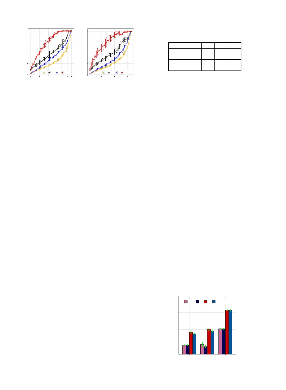
1 T ag-W eighted T opic Model F or Large-scale Semi-Str uctured Docume nts Shuangyin Li, Jief ei Li, Guan Huang, Ruiyang T an, and Rong P an Abstract —T o date , there hav e been massive Semi-Structured Do cuments (SSDs) during the ev olution of the Internet. These SSDs contain both unstr uctured f eatures (e.g., pl ain text) a nd metadata (e.g., tags). Most pre vious works focused on modeling the unstructured tex t, and recently , some other methods hav e b een proposed to model the unstructured te xt with speciﬁc tags. T o build a general model f or SSDs remains an impor tant problem in ter ms of both model ﬁtness and efﬁciency . We propose a nov el method to model the SSDs by a so-called T ag-W eighted T opic Model (TWTM). TWTM is a framew ork that lev erages both the tags and words inf or mation, not only to learn the document-topic and topic-word distributions, but al so to infer the tag-topic distributions f or text mining tasks. We present an efﬁcient variational inference method with an EM algorithm for estimating the model parameters . M eanwhile, we propose three large-scale s olutions for our model under the M apReduce distr ibuted computing platf or m f or modeling large-scale SSDs. The experimental results show the effect iveness , efﬁciency and the robustness by comparing our model with the state-of-the-art methods in document modeling, tags prediction and text classiﬁcation. We also show the perf ormance of the three distributed solutions in terms of time and accuracy on document modeling. Index T erms —semi-structured documents, topic model, tag-weighted, v ariational inf erence, large-scale, parallelized solutions ✦ 1 I N T R O D U C T I O N I N the evolution of the Internet, there have been a huge amount of documents in many web ap- plications. Such kinds of documents with both pla in text data a nd document metada ta (tags, which can be viewed as features of the corresponding document) are called the Semi-Structured Documen ts (SSDs). How to chara cterize the se mi-structured document data becomes an important issue a ddressed in many areas, s uch as information retrieval, a r tiﬁcial i ntelli- gence and d ata mining etc. The tags can be more important than the text data in document mining. For exa mple, in IMDB 1 , the world’s most popular and a uthoritative source f or movie, TV and celebrity content, each movie has lots of tags, like director , writers, stars, c ountry , language and so on, and a storyline as te x t data. Given a movie with a tag “ Dick Martin”, we may have an idea that it has a higher chance to be a comedy , without read the full text of its storyline o r watch it . A nother example is that in a collection of scientiﬁc articles, e a ch document ha s a list tags(a uthors and keywords). Before read the main text of paper , we wo uld know what it talks about after we see the authors or the k eywords that the paper provides. Many solutio ns have been proposed to deal with the semi-structured documents (e.g., SVD, LSI) , and shown to be useful in document mining [11], [ 25], [ 35], • Shuangyin Li, Jiefei Li, Guan Huang, Ruiyang T an, and Rong Pan’ s E-mails: shuangyinli@cse.ust.hk, { liji efei@mail2., huangg6@mail2., tanry@mail2., panr@ } sysu.edu. cn. Subm itted and reviewed by IEEE T ransactio ns on Knowledge and D ata Engineering (TKED). 1. http://www .imdb.com [33], e .g., text cla ssiﬁcation and structural informa- tion e xploiting. For document modeling, topic models have been used to b e a powerful method of a nalyzing and m odeling of document corpora, using Bayesian statistics and machine learning to discover the the- matic contents of untagged documents. T opic models can discover t he latent structur es in documents and establish links between them, such a s latent Dirichlet allocation (LDA) [9] . However , a s an unsupervised method, only the words in the documents are mod- eled in LDA. Thus, LDA could only treat the tags as word features r ather than a new kind of information for document modeling. T o model semi-structured documents needs to con- sider the characteristics of different kinds of objects, including word, topic, document, and tag, and the relationship among them. In this problem, topic is a kind of hidden objects, and the other three are the observations. Relative to tag, word and docu- ment are objective; tag can be either objective (e.g., author and venue information of publications) and subjective (e.g., tags in social bookmark marked by people). Similar to the topic models, we should con- sider binary relationships b e tween the pairs of the objects, including topic-word and document-topic. In addition, we may consider the b inar y relations hips, like tag-word, ta g- topic, tag-document, and tag-tag. The tag-document relations hip implies that we sh ould consider the weights of the tags in each document. The ta g-topic and tag-tag relationships c an be more complicated, thus a re difﬁcult to model. Some earlier works consider ce r tain tags. For example, the author- topic model in [31] considers the a uthorship informa- tion of the d ocuments to be modeled. In this work, we 2 don’t limit the types and number of the tags in eac h document. In an extreme case, where there is no ta g in any document, the new model may d egenerates into LDA. On the other hand, since the ta gs can be created by some people, they should be relevant to topics of the documents; however , some of them may be correlated, redunda nt, and even noisy . Therefore, the tag-topic relation ships should be general enough and we should also model the weights of the tags in each document. In the past few yea rs, researchers have proposed ap- proaches to model documents with tags or labels [26], [29], [30]. For e xample, Labeled LDA [29] a ssumes there is no latent topics and each topic is r estricted to be associated with the given labels. PLDA assumes that each topic is a ssociated with only one label [ 30]. However , both Labeled LDA a nd PLDA have implicit assumptions that the given labels should be strongly associated with the topics to be modeled or the labels are independent to each other . Another problem is that we would get i nto trou- ble when we need to de al with large-scale semi- structured d ocuments. A variety of algorithms have been used to estimate the parameters of these pro - posed topic models for mining documents, such as Monte Carlo Mar kov chain (MCMC) sampling tech- niques [1], [19], varia tional methods [3] and others methods [2], [ 32]. For sampling methods, actually , we may have to appeal to a tailored solution of MCMC [7] for a particular model, which would impede the requirem ent of convergence properties and speed, es- pecially when the corpus comprise millions of words. V ariational methods as app roximation solutions to some extent improve the learning speed. However , it would also be ineffective on lea rning speed and model accurac y when it comes to a large-scale corpus. In this pa per , we propose a framework of T ag- W eighted T opic Model (TWTM) to repr esent the text data and the va r ious tags with weights to evalu- ate the importance of the tags. Be sides lear ning the topic distributions of d ocuments and generating the topic distributions over words, the framework also infers the topic distributions of ta gs. The weights of observed tags in e ach document, which we infer from the d ataset, give us an opportunity to provide a method to rank the tags. In many web applica tions, not all the documents in the c orpora have tags. There are lots of documents only consist of words without any tags which maybe removed after data preprocessing for denoising. Only consider the weights a mong tags would not hold this c ase. T o a ddress this problem, we a lso propose a more ﬂexible model called T a g-W eighted Dirich- let Allocation (TWDA) as an extended model. It is based on TWTM, and learns the weights among a Dirichlet prior and the given tags, not just among the tags. Therefore, TWDA handles no t only the semi-structured documents, but also the unstructured documents. For the unstructur ed documents, TWDA degenerates into latent Dirichlet allocation (LDA). For hybrid corpora which consist of both the semi- structured documents and unstructured documents, TWDA can handle this complex type of corpora more effectively and easily . For the cha llenge of modeling large-scale corpora, we propose three distributed schemes for the frame- work of TWTM model in MapReduce programming framework [16]. The proposed model has four princi- pal contributions. 1) It is a novel topic modeling method to model the semi-structured documents, not only gener- ating the topic distributions over words, but also inferring the topic distributions of tags. 2) The TWTM leverages the weights a mong the observed tags in a document to eva luate the importance of the tags using a function of ta g- weighted topic assignment process. The weights are associated with the observed tags in a doc- ument providing a way to rank the ta gs. In addition, this c ould be used to predict la tent tags in the document. 3) The framework of tag-weighted process is easy to extend for many different real world appli- cations. For example, with the extended model TWDA, we can handle both the multi-tag docu- ments a nd non-tag documents simultaneously , which is very useful to p rocess some compli- cated web app lica tions. 4) Three distributed solutions for TWTM have been proposed that focus on challenges of working at a large-scale semi-structured documents in MapReduce programming framework. The rest of the paper is organized as follows. In Se c- tion 2, we ﬁrst analyze and discuss related works. In Section 3, a fter introducing the notations, we present the novel topic modeling framework of TWTM, and give the methods of lea rning a nd inference. In Sec- tion 4 , we show the e xtended model T WDA , and give the process of learning and inference. In Section 5, we will give the theoretical ana lysis to discuss the differences between TWTM a nd TWDA, comparing the other topic models. In Sec tion 6 , we propose three distributed solutions of T WTM f or a large-scale semi- structured documents. In Section 7, we present the experimental resul ts on three domains to show the performance of the proposed method in document modeling, text classiﬁcation and the e ffectiveness and efﬁciency of the three large-scale solutions on a large scale se mi-structured d ocuments modeling. W e end the paper in Section 8. 2 R E L AT E D W O R K S T opic models provide an a malgam of ideas d rawn from mathematics, computer science, and cognitive science to help users understand unstructured da ta. 3 There are many topic models proposed and shown to be powerful on document analyzing, such as in [28], [20], [9], [8], [10], [1 4], which have been applied to many areas, including document clustering and classiﬁcation [1 2], and information retrieval [3 4]. They are e x tended to many other topic models for different situation of applications in analyzing text data [21], [23], [36]. However , most of these models only con- sider the textual information and can only treat the tag information as plain text as well. TMBP [17] and cFTM [15] propose the methods to make use of the contextual information of documents for topic modeling. TMBP is a topic model with biased propagation to leveraging c ontextual information, the authors and venue. TMBP needs to predeﬁne the weights of the author and venue information on word assignment, which limits the usef ulness in real applications. The method of cFTM has a very strong assumption that ea ch word is associated with only one tag, either author or venue. In many applications, this assumption may not hold. Several models have been proposed to take ad - vantage of tags or labels, such a s Labeled LDA [29], DMR [26] and PLDA [30], or modeling relationships among severa l var iables, such as Author-T opic Model [31]. Labeled LDA [ 29] get the topic distribution for a document through picking out the several hyper- parameter components that correspond to its la bels, and dra w the topic components by the new hyper- parameter without inferring the topic distribution of labels. Labeled LDA does not assume the ex istence of a ny latent topics [30]. PLDA [3 0] provides an- other way of modeling the tagged text data, which assumes the generation topics a ssignment is limited by only one of the given tags for one word, and in the training process, PLDA a ssumes that each topic takes part in exactly one label, and may optio nally share global label present on eve r y document. In Author T opic Model, it obtains the topic distributions of authors, without giving the importance weights among the given authors in e ach document. DMR [26] is a Dirichlet-multinomial regression topic model that includes a log-linear prior on the document- topic distributions, which is an exponential function of the given features of the document. However , DMR doesn’t output the ta g weights either [ 31], which is useful for tag ranking. So in this work, we propose a tag-weighted topic modeling framework which lever ages the tag infor- mation given in a document by a list of weight values to model the topic distribution of the docu- ment. Meanwhile, f or a mixture collection of semi- structured documents and unstructured documents, we present a n extended model called tag-weighted Dirichlet Allocation which c onsiders both a Dirich- let prior and the tags by the weight va lues among them. Based on the framework of T ag-W eighted T opic Model, we also show three la rge-scale solutions under the Ma pReduce d istributed computing platform for large-scale semi-structured documents. 3 T W T M M O D E L A N D A L G O R I T H M S In this section, we will mathematically deﬁne the tag-weighted topic model ( T WT M ), and discuss the learning and inference methods. 3.1 Notation Similar to LDA [9], we formally deﬁne the following terms. Consider a semi-structured corpus, a collec- tion of M documents. W e deﬁne the corpus D = { ( w 1 , t 1 ) , . . . , ( w M , t M ) } , wher e each 2- tuple ( w d , t d ) denotes a document, the ba g-of-word representation w d = ( w d 1 , . . . , w d N ) , t d = ( t d 1 , . . . , t d L ) is the document tag vector , e a ch element of which be ing a binary tag indicator , and L is the size of the tag set in the corpus D . For the convenience of the inference in this paper , t d is expanded to a l d × L matrix T d , where l d is the number of tags in the document d . For each ro w number i ∈ { 1 , . . . , l d } in T d , T d i · is a binary vector , where T d ij = 1 if and only if the i -th tag of the document d 2 is the j -th tag of the tag set in the corpus D . In this pa per , we wish to ﬁnd a probabilistic model for the corpus D that assigns high likelihood to the documents in the corpus and other documents alike utilizing the given tag information. 3.2 T ag-W eighted T op ic Model TWTM is a probabilistic graphical model that de- scribes a process for genera ting a semi-structured document collection. In the previous topic models, a document d is typically characte r ized by a multino- mial distribution over topics, θ d , and each topic k is represented by ψ k , over words in a voca b ula ry . T ake LDA [ 9] a s an exa mple, the generative process of topic distribution of document d is assumed as f ollows. Choose θ d ∼ Dirichlet ( α ) , and choose z ni ∼ Multinomial ( θ d ) , where α is the hyperpara meter of θ d . In LDA, the topic distribution θ d is drawn f rom a hyperpa rameter α , without considering the given tags. However , the tag information should be more useful f or the generation of θ d than a Dirichlet prior . In this paper , we use ϑ d , instead of θ d , to denote the topic distribution of document d as shown in Figure 1. Let θ represent a L × K topic distribution matrix over the tag set, where K is the number of topics. Let ψ represent a K × V distribution matrix over words in the dictionary , where V is the number of words in the dictionary of D . Similar to LDA, TWTM models the document d as a mixture of underlying 2. Note th at we can sort t he tags of the documen t d by t he ind ex of the tag set of the corpus D . 4 ε d ϑ d z w N D L t η θ L × K ψ K × V π Fig. 1. Graphical model representation f or TWTM, where θ is distr ib ution matr ix of the whole tags, ψ is distributi on matr ix of words, ǫ d represents the weight vector of the tags, and ϑ d indicates the topic compo- nents for each document. π is a Dir ichlet pr ior and η is a Bernoulli pr ior . topics a nd generate s each word f rom one topic. The topic proportions ϑ d of the document d is a mixture of tag-topic distributions, not only controlled by a hyperparameter described as in LDA. The genera tive process for TWTM is given in the following procedure: 1) For each topic k ∈ { 1 , . . . , K } , draw ψ k ∼ Dir( β ) , where β is a V dimensional prior vector of ψ . 2) For each tag t ∈ { 1 , . . . , L } , draw θ t ∼ Dir( α ), where α is a K di me nsional prior vector of θ . 3) For each document d : a) For each l ∈ { 1 , . . . , L } , d raw t d l ∼ Bernoulli ( η l ). b) Generate T d by t d . c) Draw ε d ∼ Dir ( T d × π ) . d) Generate ϑ d = ( ε d ) T × ( T d × θ ) . e) For each word w di : i) Draw z di ∼ Mult( ϑ d ). ii) Draw w di ∼ Mult( ψ z di ). In this process, Dir( · ) de signates a Dirichlet d istri- bution, Mult( · ) is a multinomial distribution, and π is a L × 1 c olumn vector , a Dirichlet prior . Note that ε d indicates the weight vec tor of the observ e d tags in constituting the topic proportions of the document d , and ( ε d ) T is the tra nspose of ε d . Furthermore, ε d is drawn f rom a Dirichlet prior which obtained by the matrix multiplication of T d × π . Clearly , the result of T d × π will be a ( l d × 1 ) vector whose dimension is depended on the number of the observed ta gs in the document d . In Ste p 3, for one document d , we ﬁrst generate the document’s tags t d l using a Bernoulli coin toss with a prior probability η l , as shown in step (a). A f ter draw out the ε d , we generate the ϑ d through ε d , T d and θ . The remaining part of the gener a tive process is just familiar with LDA [9]. As shown above, in TWTM, we intr oduce a novel way to model the topic pro- portions of semi-structured document by document- special tags and text data. The key discussed in this paper is the tag’s weight topic assignment by which ϑ d is generated through ε d , T d , and θ , which provides an effective and direct method to infer the weights of the tags. 3.3 T ag-W eighted T op ic Assignment As we assume that all the observed tags in the docu- ment d make contributions to infer the topic distribu- tion ϑ d of the document, it is expected that different tags works corresponding to their own weights. For example, in some blog application, a blog has ta gs of an author , a b log’s da te, a blog category and a blog’s url. Clea rly , compared to other tags, the tag of the author plays the most important role in constitutin g the topic components of the blog. The function of how to leverage the tag information or contextual to infer topic d istribution of a document is deﬁned as follows: ϑ ← − f ( t 1 , · · · , t l ) , where f ( · ) is the way of ma king use of the tag information. T opic models using tag information or contextual take adva ntage of the different f ( · ) in the past. In TWTM, we a ssume that ϑ d is made up by all the observed tags with their own weights. Figure 1 shows that how TWTM works in a prob- abilistic grap hica l model. As shown in Figure 1, ϑ d is controlled by two sides, the topic distributions over tags θ , and the weights of the given tags of the document d . It is important to distinguish TWTM from the Author-T opic M odel [3 1]. In the author-topic model, the words w is chose only by one of the given tags’ distribution, while in TWTM, for word w , all the observed tags in the d ocument would make the contributions. The f ( · ) in the proposed model is a ssumed as this, for the document d , f ( ϑ d ) = ( ε d ) T × T d × θ , where the linear multiplication of ( ε d ) T , T d and θ maintains the condition of P K k =1 ϑ d k = 1 without normalization of ϑ d , since ε d and θ satisfy l d X i =1 ε d i = 1 , K X k =1 θ lk = 1 . Firstly , we pick out the topic distributions of the given tags in the document d from θ by T d × θ , where T d is a l d × L matrix and θ is a L × K ma trix. Here we deﬁne Θ d = T d × θ , where the Θ d is a l d × K topic distribution matrix of the given tags in d as sub-components of θ . Secondly , ε d is the weight vector of the observ e d tags in d , and e ach dimension of ε d represents the weight or importance associated to the corresponding tag. Thus, ϑ d is mixed b y Θ d with corresponding weight values. ϑ d = ( l d X i =1 ε d i Θ d i 1 , . . . , l d X i =1 ε d i Θ d ij , . . . , l d X i =1 ε d i Θ d iK ) . 5 ε d ξ γ d z N M Fig. 2. Graphical model representation of the varia- tional distr ib ution used to approximate the pos terior in TWTM. W ith ϑ d , TWTM generates a ll the words in the document d with the assumption of bag-of- words. Based on the above framework, we can deﬁne a special topic assignment function f ( · ) in an extended model for a real world a p p lica tion. 3.4 Inference f or TWTM In the topic models, the key inferential problem that we need to solve is to compute the posterior d istri- bution of the hidden variab le s given a document d . Given the document d , we can e a sily get the posterior distribution of the latent variables in the proposed model, as: p ( ε d , z | w d , T d , θ , η , ψ, π ) = p ( ε d , z , w d , T d | θ , η , ψ , π ) p ( w d , T d | θ , η , ψ, π ) . (1) In Eq. (1), integrating over ε and summing out z , we easily obtain the marginal distribution of d : p ( w d , T d | η, θ , ψ , π ) = p ( t d | η ) Z p  ε d | ( T d × π )  · N Y i =1 K X z d i =1 p ( z d i | ( ε d ) T × T d × θ ) p ( w d i | z d i , ψ 1: K ) dε d . In this work, we make use of mean-ﬁeld variational EM algorithm [4] to efﬁciently obtain an a pprox- imation of this posterior d istribution of the latent variables. In the mean-ﬁeld variational inference, we minimize the KL divergence between the variational posterior probability and the true posterior probabil- ity through by maximizing the e vidence lower bound (ELBO) L ( · ) [8]. For a single document d , we obtain the L ( · ) using Jensen’s inequality: L ( ξ 1: l d , γ 1: K ; η 1: L ,π 1: L , θ 1: L , ψ 1: K ) = E [log p ( T 1: l d | η 1: L )] + E [log p ( ε d | T d × π )] + N X i =1 E [ log p ( z i | ( ε d ) T × T d × θ )] + N X i =1 E [ log p ( w i | z i , ψ 1: K )] + H ( q ) , where ξ is a l d -dimensional Dirichlet pa rameter vec- tor a nd γ is 1 × K vector , both of which are variational parameters of v a riational distribution shown in Fig- ure 2, and H ( q ) indicate s the entropy of the variational distribution: H ( q ) = − E [log q ( ε d )] − E [log q ( z )] . Here the exception is taken with respect to a va ri- ational distribution q ( ε d , z 1: N ) , and we choose the following fully fa ctorized d istribution: q ( ε d , z 1: N | ξ 1: L , γ 1: K ) = q ( ε d | ξ ) N Y i =1 q ( z i | γ i ) . The dimension of para mete r ξ is changed with dif- ferent documents. It could be difﬁcult to compute the expected log probability of a topic a ssignment by the way of tag-weighted topic assignment used in TWTM. Then, we maximize the lower bound L ( · ) with respect to the varia tional pa rameters ξ and γ , using a variational expecta tion-maximization(EM) procedure as follows. 3.4.1 V ar iational E-step W e ﬁrst maximize L ( · ) with respect to ξ i for the document d . M aximize the terms which contain ξ : L [ ξ ] = l d X i =1 ( L X l ′ =1 π l ′ T d il ′ − 1)(Ψ( ξ i ) − Ψ( l d X j ′ =1 ξ j ′ )) + N X i =1 K X k =1 γ ik · l d X j =1 log θ ( j ) k ξ j / l d X j ′ =1 ξ j ′ − l og Γ( l d X i =1 ξ i ) + l d X i =1 log Γ( ξ i ) − l d X i =1 ( ξ i − 1)(Ψ( ξ i ) − Ψ( l d X j ′ =1 ξ j ′ )) , (2) where Ψ( · ) denotes the digamma function, the ﬁrst derivative of the log of the Gamma function. Here we use gra dient de scent method to ﬁnd the ξ to make the maximization of L [ ξ ] . Next, we maximize L ( · ) with respect to γ ik . Add ing the Lagr a nge multipliers to the terms which contain γ ik , taking the derivative with respect to γ ik , and setting the d e rivative to zero yields, we obtain the update equation of γ ik : γ ik ∝ ψ k,v w i exp { l d X j =1 log θ ( j ) k ξ j P l d j ′ =1 ξ j ′ } , (3) where v w i denotes the index of w i in the dictionary . In E- step, we update the ξ and γ for e ach document with the initialized model para meters. For the reason of different d ocument with different number of ta gs, we have to keep all the ξ updated by each d ocument for the M- step estimation. 3.4.2 M-step estimation The M-step needs to update four parameter s: η , the tagging prior probability , π , the Dirichlet prior of the tags’ weights, θ , the topic distribution over all ta gs in the corpus, and ψ , the probability of a word under a topic. Because each document’s tag-set is observed, the Bernoulli prior η is unused included for model completeness. For a given corpus, the η i is estimated by ad d ing up the number of i -th tag which appears in the corpus. 6 For the document d , the terms that involve the Dirichlet prior π : L [ π ] = log Γ   l d X i =1 ( T d × π ) i   − l d X i =1 log Γ  ( T d × π ) i  + l d X i =1  ( T d × π ) i − 1    Ψ( ξ i ) − Ψ( l d X j =1 ξ j )   , (4) where ( T d × π ) i = P l d i =1 P L l =1 π l T d il . W e use gradient descent method by taking derivative of Eq. (4) with respect to π l on the corpus to ﬁnd the e stimation of π . T o ma x imize with respect to θ and ψ , we obtain the following update equations: θ lk ∝ D X d =1 N X i =1 γ d ik ξ d l t d l P L l =1 ( ξ d l t d l ) , (5) and ψ kj ∝ D X d =1 N X i =1 γ d ik ( w d ) j i . (6) W e provide a detailed derivation of the varia tional EM algorithm for T WT M in Appendix A. And we show the varia tional expectation maximization ( E M) procedure of TWTM in Algorithm 1. Algorithm 1 The variational e x pectation maximiza- tion (EM) a lgorithm of TWTM 1: Input: a semi-structured corpora including totally V unique words, L unique tags, and the expected number K of topics. 2: Output: T opic-word distributions ψ , T ag-topic dis- tributions θ , π , topic distribution ϑ d and weight vector ε d of each tra ining document. 3: initialize π , and initialize θ and ψ with the con- straint of P K k =1 θ lk equals 1 and P V i =1 ψ ki equals 1. 4: repeat 5: for each document d do 6: update ξ d with Eq. (2) using gradient descent method. 7: update γ ik with Eq. (3). 8: end for 9: update π with Eq. (4) using gra dient desce nt method. 10: update θ by Eq. (5). 11: update ψ by Eq. (6). 12: until convergence 4 T AG - W E I G H T E D D I R I C H L E T A L L O C AT I O N In a real world ap p lication, a corpus is very likely to contain both semi-structured documents and un- structured documents. Many documents in the corpus have no tags, just with unstructured text data. In this case, TWT M does not work, which genera tes the topic distribution of a document by le v e raging ε d ϑ d λ µ z w N D L t η θ L × K ψ K × V π Fig. 3. Graphical model representation for T WD A, where µ is a Dirichlet pr ior of λ . the weights a mong the observed tags. Our proposed solution to the problem is to add a Dirichlet prior to the topic distribution ϑ d , which means that we lea rn the weights among the Dirichlet pr ior a nd the given tags, not just among the ta gs. W e call this solution T ag- W eighted Dirichlet Allocation (TWDA). When han- dling the unstructured documents in a hybrid corpus, TWDA de generates into LDA [9] which just draws the topic proportions for a document from a Dirichlet distribution. As an extended model of TWTM, TWDA uses the same par ameter notations. Unlike TWTM, f or the convenience of the inference in TWDA, t d is expa nde d to a l d × ( L + 1) ma trix T d , where l d is one more than the number of the given tags in the document d (For example, if the document d has ﬁve tags, l d is six). For each row number i ∈ { 1 , . . . , l d } in T d , T d i · is a binary vector , where T d ij = 1 if and only if the i -th tag of the document d is the j -th tag of the tag set in the corpus D . Note that, we set the last dimension of the last row in T d to 1 , and the other dimensions of the last row equal to 0 f or all documents. The d e tail of the above setting will be shown later . TWDA deﬁnes a Dirichlet prior µ over a latent topic distribution of a document, a nd mixes the latent topic proportion with these topic distributions of the given tags by importance or weight (tag-weighted) to form the ﬁnal topic distribution of the document. Figure 3 shows the graphical model representation of TWDA, and the generative process for TWDA is given in the following procedure: 1) For each topic k ∈ { 1 , . . . , K } , draw ψ k ∼ Dir( β ) , where β is a V dimensional prior vector of ψ . 2) For each tag t ∈ { 1 , . . . , L } , draw θ t ∼ Dir( α ), where α is a K di me nsional prior vector of θ . 3) For each document d : a) Draw λ ∼ D ir ( µ ) . b) Generate T d by t d . c) Draw ε d ∼ Dir ( T d × π ) . d) Generate ϑ d = ( ε d ) T × T d × ( θ λ ) . e) For each word w di : 7 i) Draw z di ∼ Mult( ϑ d ) . ii) Draw w di ∼ Mult( ψ z di ) . Note that, L is the number of ta gs appeared in the corpora and K is the number of topics. Different from TWTM, here π is a ( L + 1) × 1 column vec tor and µ is a K × 1 column vector . Both of them a re Dirichlet prior . λ is a 1 × K row vector which is dra wn f rom µ . ( ε d ) T is the transpose of ε d , and ε d is drawn from a Dirichlet prior which obtained by the matrix multiplication of T d × π . C le a rly , the result of T d × π will be a ( l d × 1 ) vector whose dimension is depended on the number of the observed tags in the document d . Note that, l d is one more than the number of tags given in d as we described above. In other words, we treat the λ as a topic distribution of one latent tag, the Dirichlet pr ior µ . Ea ch document is controll ed by a latent tag, that is the sa me idea both T WDA and La tent Dirichlet Allocation (LDA). The form of ( θ λ ) is the augmented matr ix of θ and λ , which represents that we add the vector λ to the matrix θ a s the last row , so ( θ λ ) becomes a ( L + 1 ) × K matrix. As we show above, T d is the matrix form of the given tags in the document d , and the last row of T d is a binary vector , of which only the last dimension equals to 1 a nd the others e qual 0. Here we deﬁne Θ d = T d × ( θ λ ) . Clearly , Θ d is a l d × K matrix, whose last row is λ . Actua lly , the purpose of Θ d is to pick out the rows corresponded to the tags appeared in d from tag-topic distribution matrix θ . The key idea of tag-weighted Dirichlet allocation is to model the topic proportions of semi-structured documents by document-special tags a nd text data. Different from LDA , the topic proportion of one doc- ument assumed in this model is controlled not only by a Dirichlet prior µ , but a lso by all the observed tags. The way to generate the normalized topic distribution of the document d is that we mix both Dirichlet allo- cation and tags information thr ough a weight vector ε d . T hus, we use the f unction f ( · ) of topic assignment to obtain the topic distribution of d by f ( ϑ d ) = ( ε d ) T × T d × ( θ λ ) . It is worth to note that the ε d is dra w by a Dirichlet prior π , ea ch row of θ is draw by a Dirichlet prior α , a nd λ is d raw by a Dirichlet prior µ , so ε d and θ satisfy l d X i =1 ε d i = 1 , K X k =1 θ lk = 1 , and K X k =1 λ k = 1 . Therefore, the linear multiplication of ( ε d ) T , T d , θ and λ maintains the condition of P K k =1 ϑ d k = 1 without normalization of ϑ d . W ith ϑ d , the topic proportions of the document d , the remaining part of the generative process is just familiar with L DA. ε d ξ ρ λ γ d z N M Fig. 4. Graphical model representation of the varia- tional distr ib ution used to approximate the pos terior in TWD A. 4.1 Inference f or TWD A In TWDA , we treat π , µ , η , θ and ψ as unknown constants to be estimated. Similar to TWTM, the marginal distribution of d is not efﬁciently computable as follows: p ( w d , T d | η, θ , ψ , π , µ ) = p ( t d | η ) Z p  ε d | ( T d × π )  · p ( λ | µ ) N Y i =1 K X z d i =1 p ( z d i | ( ε d ) T × T d × ( θ λ )) · p ( w d i | z d i , ψ 1: K ) dε d . In this case, W e also use a variational expectation- maximization (E M ) procedure to carry out approxi- mate maximum likelihood estimation of TWDA. 4.1.1 V ar iational inference In TWDA, we use the followin g f ully factorized dis- tribution as shown in Figure 4: q ( ε d , λ d , z 1: N | ξ 1: L , ρ 1: K , γ 1: K ) = q ( ε d | ξ ) q ( λ d | ρ ) N Y i =1 q ( z i | γ i ) , and the entropy of the variational d istribution will be H ( q ) = − E [log q ( ε d )] − E [log q ( λ )] − E [log q ( z )] . For the va riational para meter ξ , we take the terms which contain ξ out of the evide nce lower bound (ELBO) L ( · ) of TWDA to form L [ ξ ] , and we use gradient descent method to ﬁnd the ξ to make the maximization of L [ ξ ] : L [ ξ ] = l d X i =1 ( L +1 X l ′ =1 π l ′ T d il ′ − 1)(Ψ( ξ i ) − Ψ( l d X j ′ =1 ξ j ′ )) + N X i =1 K X k =1 γ ik · l d X j =1 C ( j ) k ξ j P l d j ′ =1 ξ j ′ − l og Γ( l d X i =1 ξ i ) + l d X i =1 log Γ( ξ i ) − l d X i =1 ( ξ i − 1)(Ψ( ξ i ) − Ψ( l d X j ′ =1 ξ j ′ )) , (7) where C ( j ) k = ( log θ ( j ) k j ∈ { 1 , · · · , l d − 1 } Ψ( ρ k ) − Ψ( P K j ′ =1 ρ j ′ ) j = l d , and Ψ( · ) denotes the digamma function, the ﬁrst derivative of the log of the Gamma function. 8 In pa r ticular , by computing the d erivatives of the L ( · ) a nd setting them equal to zero, we obtain the following pair of update equations for the va riational parameters ρ d and γ ik : ρ i ∝ µ i + N X n =1 γ ni · ξ l d P l d j =1 ξ j , (8) γ ik ∝ ψ k,v w i exp { l d X j =1 C ( j ) k ξ j P l d j ′ =1 ξ j ′ } , (9) where v w i denotes the index of w i in the dictionary . In the E-step, we update the va riational parameter s ξ , ρ and γ for eac h document with the initialized model parameters. W e show the detailed derivation of the variational par ameters for TWDA in A ppendix B. 4.1.2 Model P arame ter Estimation There are four model parameters tha t nee d to estimate in M-step, π , the Dirichlet prior of the tags’ weights, θ , the topic distribution over all tags in the corpus, ψ , the probability of a word under a topic, and µ , a Dirichlet prior of model. In TWDA, we can estimate π , θ and ψ a s same as in TWTM. Different from TWTM , TWDA has a n extra Dirichlet prior µ . The involved te rms of µ are: L [ µ ] = D X d =1 (log Γ( K X j =1 µ j ) − K X i =1 log Γ( µ i ) + K X i =1 ( µ i − 1)(Ψ( ρ d i ) − Ψ( K X j =1 ρ d j ))) . (10) W e can invoke the linear-time Newton-Raphson algo- rithm to e stimate µ a s same as the Dirichlet pa rameter described in L DA [ 9]. In the variational e xpectation maximization (EM ) procedure of TWDA, we update the var ia tional pa- rameters ξ d , ρ a nd γ ik with Eqs. (7), (8) and (9) respectively in the E-step. In the M -step, besides the update of π , θ and ψ , we also update µ with Eq. (10) by Newton-Raphson algorithm. The deta iled derivation of the model pa rameter estimation in TWDA is shown in Appendix B. 5 A N A L Y S I S O F T W DA In TWDA, we introduce a bette r way to d irectly model the semi-structured documents and unstructured doc- uments by adding a latent tag to each documents, which the topic distribution of a d ocument is con- trolled by the observed tags and one latent tag. In LDA, the topic distribution of a document is drawn from a hyperpar ameter , without considering the given tags, a nd while in TWTM, the topic distribution is controlled by a list of given tags with correspondin g weight values. The main difference among the models which handle the unstructured text (e.g., L DA and CTM [7]) or the semi-structured documents (e.g., A T M [31], Label-L DA [ 29], DMR [26] and PLDA [ 30]) is the function that how to genera te the topic distribution of a document, or , in other words, the assumption that what distribution the topic of a document f ollows. In TWDA, the topic p roportion s ϑ d for a document d is obtained by the following function: ϑ d = ( ε d ) T × T d × ( θ λ ) When we ignore the ta gs in a document, the T d in Eq. (5) becomes a b inar y row vector and the last dimension equals to 1 and the others are 0. In this case, ( θ λ ) is simpliﬁed to λ : ϑ d = ( ε d ) T × T d × ( θ λ ) = λ. The topic distribution of d is simpliﬁed to λ , and as we shown above, λ is dra w by a Dirichlet pr ior µ . It means that the topic proportio ns for the document d as a draw from a Dirichlet distribution which is the basic assumption of LDA [9]. In others words, when handling the unstructur ed documents, TWDA degenerates into LDA. In other wor ds, the topic distribution of a docu- ment in TWTM is the weighted avera ge of the topic distributions of the given ta gs, and to some extent, it is a linear relation between the topic distribution of a document and the tags. While, in TWDA, with the addition of the Dirichlet pr ior µ , which is equal to generate a latent ta g for ea ch document with a special topic distribution, it is a non-linear topic generation procedure in ea ch d ocument. 6 L A R G E S C A L E S O L U T I O N S Currently , many web a pplications a ppear with large scale tagged documents, and highlight the issues of large scale semi-structured documents in many areas. In this paper , we propose and compare three dif- ferent distributed methods based on the fr a mework of TWTM, which focus on the challenge of working at a large scale, in the M a pReduce programming framework. Solution I The ﬁrst solution is a tailored parallel a lgorithm for TWTM. The lear ning and inference of the proposed model are based on variational method with an EM algorithm. Thus, we design a pa rallel algorithm for TWTM using M apReduce programming fra mework. As shown above, we need to update the global parameters π , θ , a nd ψ for a corpus. Every document has associated with the corresponding variational pa- rameters ξ and γ . The mapper computes these varia- tional pa rameters for each document a nd uses them to generate the sufﬁcient sta tistics to update π , θ , and ψ . 9 And the reducer updates the global parameters π , θ , and ψ . 1) Mapper : For each document d , we compute γ d using the upd ate equation Eq. (3) and obtain ξ d by Eq. (2). The sufﬁcient statistics are kept for each document. 2) Reducer : The Reduce f unction adds the value to the global p a rameters θ and ψ using the sufﬁcient sta tistics as in Eqs. (5), and (6). 3) Driver : The driver program marshals the entire inference process. At the b e ginning, the dr iver initializes all the model par ameters K , L , θ , ψ , and π . The topic number K is user speciﬁed; the number of tags L is determined by the data; the initial va lue of π is given by the user , θ and ψ is ra ndomly initialized. After each MapReduce iteration, the driver normalizes the global θ a nd ψ . Note that, because π is a global parameter over the corpus, we have to update π at the end of ea ch iteration in driver . However , this will lead to a large scale data migration to compute the π by Eq. (4), since π is associated with each document and different documents have different tags which affect the differ- ent dimensions in π . T he whole corpus data would migrate to the single driver node. This could generate a bottleneck in the driver . Solution II On a ccount of the bottleneck in Solution I, we op- timize the calculation of π through a n approximate method as the Solution II. The MapReduc e procedure of Solution II is as follows. 1) Mapper : For each document d , we compute γ d and ξ d by E qs. (2) a nd (3) and the sufﬁcient statistics for upd ating θ and ψ . Different with Solution I, we obtain a π s for each map data split s by Eq. (4). 2) Reducer : The Reduce f unction adds the value to the global p a rameters θ and ψ using the sufﬁcient sta tistics as in Eqs. (5), and (6). 3) Driver : In the driver function, we only need to compute an average of π s , s ∈ (1 , · · · , S ) where S is the total number of mapper in the cluster . The d r iver a lso normalizes the global θ and ψ for next itera tion. Solution II is an approximate solution of TWTM , which computes the π s for each mapper and takes their average a s the solution of π to avoid the large scale data migration. Solution III As shown in E q. (4), π l , l ∈ (1 , · · · , L ) is only as- sociated with the d ocuments who contain the l th tag. Thus, before running TWTM, we can cluster the documents into seve ral clusters with the condition that the documents which contain one or a plurality of the sa me tag should be in the same cluster . It means that the documents are divide d into the mu- tually independe nt space by the tags. W e show the detailed process of the clustering in Appendix C. The MapReduce procedure of S olution III is the following procedure. 1) Mapper : The input of mapper is clusters. For each cluster , we obtain a π c for the cluster c , c ∈ (1 , · · · , C ) , where C is the number of doc- ument clusters, which is the sufﬁcient statistics for updating θ and ψ . 2) Reducer : The Reduce f unction adds the value to the global p a rameters θ and ψ using the sufﬁcient sta tistics as in Eqs. (5), and (6). 3) Driver : In the driver , we update θ and ψ . Note that there is no need to recompute π , and we combine all the π c to obtain the ﬁnal π for current itera tion. Solution III is a n exact solution for TWTM, and it is equivalent to Solution I when the documents are a ll belong to one cluster . However , Solution III provides a more efﬁcient method than Solution I, and this depends on the result of document clustering, which would be a nther bottleneck in some real ap plications. Although Solution II is a n approximate method f or modeling the semi-structured d ocuments, it effec- tively avoids the b ottleneck brought by Solution I and Solution III. The e x periment results in Section 7 show that Solution II works better than Solution I and Solution III. It is worth note that all the solut ions need to iterate the Map Red uc e procedure in driver function until convergence or maximum number of iterations is reached. In Se ction 7 , we show the e x p erimental results about the comparisons of the three solutions on document modeling a nd efﬁciency . 7 E X P E R I M E N TA L A N A L Y S I S 7.1 Experiment Settings In the e xperiments of this work, we used three semi-structured corpora. The ﬁrst document c ollection is the d a ta from Internet Movie Databa se (IMDB). The data set includes 12,0 91 movie storylines, 52,274 words after removing stop words, a nd 3,6 54 tags. These movies belong to 2 9 genres. And the tags we used contain directors, stars, time, and movie key- words. The second one consists of technical papers of the Digital B ibliography and Libra r y Project (DBLP) data set 3 , which is a collection of bibliographic infor- mation on major computer science journals and pro- ceedings. In this pa p e r , we use a subset of DBLP that contains abstra cts of D =27,43 5 pa pers, with W =70,062 words in the vocabulary and L =6,256 unique tags. The tags we used in DBLP include authors and 3. http://www .informatik.uni-trier .de/ ∼ ley/db/ 10 6000 7000 8000 10 20 50 100 150 200 # of T opics Perplexity CTM LDA TWDA TWTM (a) TWTM, TWDA, L DA and CTM 5000 7500 10000 12500 10 20 50 100 150 200 # of T opics Perplexity A TM CorrLDA CTM DMR LDA TWDA TWTM (b) TWTM, TWDA, DMR, A TM, CorrLDA, L DA and CT M 0 1000 2000 3000 4000 1021 2041 # of T opics Perplexity PLDA TWDA TWTM (c) TWTM, TWDA and PLDA Fig. 5. P erplexity results of diff erent models on IMDB cor pora. LDA and CTM only use the words when training in (a), and add the tags as the word f eatures during the training process in (b). keywords. The last corpus we used contains about 967,0 12 W ordpress blog posts 4 from Kaggle 5 . In the corpus, there are 163 ,504 tags and 2,59 2,562 words. W e used this corpus to test the effectiveness and performance of T WT M over a large scale dataset. W e implemented the three distributed methods of TWTM using Hadoop 1.1 .1 and ran all experiments on a cluster containing 7 physical nodes; each node has 4 cores and 8 threads, a nd could be conﬁgured to run a maximum of 7 ma ppers and 7 reducers of tasks. W ith the conﬁguration, we build d ifferent scales distributed environments by setting the maximum of mappers used in each node. W e ha v e released the codes on GitHub 6 including TWTM, T WDA and the three distributed solutions using the Hadoop pla tform. 7.2 Results on Documents Modeling In order to evaluate the generalization capability of the model, we use the perplexity score that described in [9]. For a test set of D documents, the perplexity is: per pl exity = exp ( − P D d log p ( w d ) P D d N d ) , where a lower perplexity score represents better doc- ument modeling pe r formance. There are two parts of the exper iments. First, W e trained four latent var iable models including LDA [9], CTM [ 7], TWTM and TWDA, on the corpora of a set of movie documents in IMDB, to compare the generalization perf ormance of the four models. In this part, LDA a nd CTM trains te xt data without taking advantage of tag information. W e removed the stop words and conducted expe r iments using 5- f old cross- validation. Figure 5(a) demonstrates the pe r plexity results on the IMDB data set. Clearly , TWTM and TWDA ex cel both CTM and LDA signi ﬁcantly and consistently . 4. http://wordpress.com 5. http://www .kaggle.com/c/predic t-wordpress-l ikes/data 6. https://github.com/Shuangyinli Second, in order to compare the per formance of TWTM and TWDA with other topic models which take advanta ge of the tag information, we trained TWTM, TWDA, DMR 7 , PLDA 8 , Author T opic Model (A TM) [3 1], CorrLDA[6], CTM , and LDA on the set of movie d ocuments in IMDB and computed the perplexity on test data set. Since CTM and LDA c ould not handle corpus with tags e asily , in this e x periment, we treated the given tags as wor d features for them. In CorrLDA, we used the tags in each document to represent the image segments, so that the CorrLDA can handle the SSDs. Figure 5(b) demonstrates the perplexity results of the six models on the IMDB data. The experiment results shows that TWTM and TWDA are bette r than the other models, and when T increases, CorrLDA, DMR, CTM and LDA are running into over-ﬁtting, while the trend of TWTM and TWDA keeps going down and the per p lexity is signiﬁcantly lower than those of the baselines. As PLDA [30] assumes that one of tags may op- tionally denote as a tag “latent” present on eve ry document d , thus, we trained PLDA, TWTM and TWDA over 1021 and 2041 topics on IM DB data set with 1020 tags, since in PLDA, eac h latent topic takes part in exactly one tag in a c ollection. A s shown in [30], PLDA builds on Labeled LDA [29], a nd when it set one latent topic a nd one topic f or ea ch tag, it is ap- proximately equivalent to Labeled LDA. For this ca se, we trained PLDA over 1 021 topics. Figure 5 (c) shows the per plexity results of TWTM, T WDA and PLDA. Note that TWDA has less mean squared error (M SE) than TWTM . As the results of Figure 5 shown, TWTM and TWDA both work well c ompared with the other topic models which make use of tag information. 7.3 Results on T ags prediction In this section we use TWDA to d emonstrated the performance of our works on the tags prediction by 7. W e used the Mallet code (htt p://mallet.cs.umass.edu/). 8. W e used the code in Stanford T opic Modeling T oolbox (http://www-nlp.stanford.edu/softwar e/tmt/tm t-0.4/). 11 0.00 0.25 0.50 0.75 1.00 100 400 8001000 1500 2000 2500 3000 3300 Rank Recall A TM CorrLDA DMR TWDA (a) K=100 0.00 0.25 0.50 0.75 1.00 100 400 8001000 1500 2000 2500 3000 3300 Rank Recall A TM CorrLDA DMR TWDA (b) K=200 Fig. 6. Prediction r esults of TWDA , DMR and A T M for authors on D BLP cor pora. W e s et the number of topic in the cor pora to be 100 in (a) and 200 in (b). process the p a per collection in DBLP . In addition to predicting the tags given a document, we evaluate the ability of the proposed model, compared with A TM, DMR and CorrL DA, to predict the tags of the document conditioned on words in the d ocument. In this pa rt, we treat the authors of ea ch pape r as the ta gs, and the abstra ct as the word fea tures, and we predict the authors of one paper by modeling the pap er a bstract document d ata using A TM, DMR, CorrLDA, and TWDA. For e ach model, we evaluate the likelihood of the authors given the word fea tures in a document, and rank each possible author by the likelihood function of the author . First, for each model, we can get the topic distribution over a test document d test given one a uthor a . Then, we evalua te the p ( d test | a ) for d test over each a uthor a in the tags(authors) set by p ( d test | a ) = N Y i ( X z p ( z | a ) p ( w i | z )) . For CorrLDA, we let authors represent image regions, and used p ( d test | reg ion ) shown in [ 6] to evaluate the likelihood of a author given a document. For DMR and A TM, the method which deﬁne p ( d test | a ) is shown a s [26]. Note tha t the likelihoods for a given a uthor over a document are not necessarily comparable among the topic models, however , what we are interested in is the ranking a s sa me as [26]. W e trained the three models on DBLP data set using 5-fold cross-validation and shows the recall when the topic in the corpora is set to be 100 and 200. Results are shown in Figure 6( a) and Figure 6(b). TWDA ranks authors consistently higher than the other models. 7.4 Results on Feature Construction for Classiﬁ- cation The next e x periment is to test the classiﬁcation perf or- mance utilizing feature sets generated by TWDA and other baselines. For the base c la ssiﬁer , we use LIBS VM [13] with Gaussian kernel and the d e fault para meters. For the purpose of comparison, we trained four SVMs T ABLE 1 Classiﬁcation results of diff erent features on F1-score F1-scor e @1 @3 @5 TFIDF 0.5 0.41 0.39 LDA+TFIDF 0. 5 0.42 0.39 TWDA 0.57 0.5 0.47 TWDA+TFIDF 0.58 0.5 0.47 on tf- idf word features, f eatures induced by a 30- topic LDA model and tf-idf word features, features generated by a TWDA model with the same number of topics, a nd fea tures induced by a 30-topic TWDA model and tf-id f word f eatures respectively . In these experiments, we conducted multi-class classiﬁcation experiments using the IMDB da ta set, which contains 29 genres. W e calculated the evalua- tion metrics @1, @3 and @5 with the provided class tags of movies’ genres, using 5-fold cross-validation. W e report the movie cla ssiﬁcation per f ormance of the different methods in Figure 7, where we see that there is signiﬁcant improvement in classiﬁcation perfor- mance when using LDA a nd TWDA comparing with only using tf- id f features, and TWDA outperforms both LDA and tf-idf in terms of @1 , @3 and @5. In order to show the classiﬁcation performance better , we also calculated the e valuation metrics F- Measure ( F1-score). The results of F-Mea sure is re- ported in T able 1. TWDA provides substantially better performance on F-M easure. 7.5 Results on Model Robustness W e demonstrated the perf orma nce of our work on model robustness in this part of e xperimental a nal- ysis. In this part, we measured and compared the perplexity when we added noise tags information to the test documents using DBLP data set. Respectively , we randomly added 20 % , 40% , 50% , 80% and 100% noise ta gs into a test document and then ca lculated the per plexity . For e xample, if a paper document in DBLP has ﬁve authors, adding 20% noise is that we randomly selected one author from the author set of 0.5 0.6 0.7 0.8 @1 @3 @5 Precision LDA+TFIDF TFIDF TWDA TWDA+TFIDF Fig. 7. Class iﬁcation results of different features on @1, @3 and @5 with 5-fol d cross- val idation. 12 the DBLP corpora and added into the paper a s a noise author . In some real-world applica tions, the nois e tags ap- peared in a document may have some relevance to the real tags. So in this expe r iment, we selected the noise ta gs f rom the author-tag set to meet the real applications to some ex te nt. In this exper iment, the DBLP corpora c ontains more than 6,0 00 tags, the noise tags we ad ded into a test document would be ver y sparse for the whole tag set in the corpora. So, we added the different percentages noise tags into the test document to show the trend of perplexity a s the noise content increases. Figure 8 shows that both TWDA a nd A TM have a more stead y trend as the noise leve l increases, compared with DMR. T able 2 shows some examples about the weights between the original tags a nd noise tags. The red tags are the noise ad ded into the test data, and the values behind are the weights among the tags we inference f rom the TWDA model. Note that, we show ed the weight values af ter normalized. As the results shown, TWDA has a good performance on model robustness, f or the weight values of the noise ta gs are much smaller than the other original tags. In some applications, we can use the proposed model to rank the tags given in a document, which would be a good a pproach to tag recommendation a nd annotation. 7.6 Results on Large-scale Datasets W e demonstrated the performance of the three pro- posed parallelized solutions of TWTM for a large- scale da taset from tra ining time and accuracy on document modeling, which are suitable for TWDA as well. Firstly , we measured and compared the training time of Solutions I, II and III using the W ordpress blog data set with the same system setting a nd model pa- rameters. W e used a doc-indexed sparse storage mode for the matrix of ξ -document, for the matrix would be ver y huge over a la rge scale da ta set. Figure 9(a) shows the performance on the avera ge tra ining time 2500 5000 7500 10000 12500 0.0 0.2 0.4 0.5 0.8 1.0 % of noise Perplexity A TM DMR TWDA (a) K=100 4000 8000 12000 16000 0.0 0.2 0.4 0.5 0.8 1.0 % of noise Perplexity A TM DMR TWDA (b) K=200 Fig. 8. The Results of adding noise to diff erent mod- els(A TM, DMR and TWD A). (a) set K=100, and (b) set K=200. Steady trending means a good performance on model rob ustness. T ABLE 2 Some e xamples of the nor malized wei ghts among the original tags and noise tags. The noise tags are in red, and the n umbers are the corresponding w eight v alues. “Bug isolation via remote program sampling [24]” Ben Liblit: 0.185 Alex A iken: 0.2257 aAlice X. Zheng: 0.228 Michael I. Jordan: 0.349 K. G. Sh in: 0.01 “W eb question answering: is more always bett e r? [18]” Susan Dumais: 0.986 Michele Ban k o: 0.0032 Eric Brill: 0.0038 Jimmy Lin: 0.0038 Andrew Ng: 0.0024 R. Katz: 0.00018 “Contextual search and name d isambiguation in email using graphs [27]” Einat Minkov: 0.425 W illiam W . Cohe n : 0.342 Andrew Y . Ng: 0.128 J. Ma: 0.033 D . Ferguson: 0.07 “A S parse Sampling Algorithm for Near-Optimal Planning in Large Markov Decision Processes [22]” Michael Kearns: 0.296 Y ishay Mansour:0.166 Andrew Y . Ng: 0.31 J. Blythe : 0.089 B. Adida: 0.027 P . J. Modi: 0.1 “The nested Chinese restaurant process and bayesian nonparametric inference of topic [5]” David M. Blei:0.46 Thomas L . Grifﬁths:0.186 Michael I. Jordan:0.225 B. Cliffor d:0.031 R. Szeliski:0.048 X. W ang:0.05 per iteration of the three solutions compared with the standard TWTM as the baseline, when we set the number of topic K = 10, 20 and 5 0 respectively . Secondly , W e sampled the training dataset from the W ordpress corpus with different sa mple ratios, 0.1, 0.3, 0.6 , 0.8 and 1.0, to show the performance of running time by different size of training dataset. In addition, we limited the maximum number of Mappers in the conﬁguration when we tra ined the 0 2500 5000 7500 10 20 50 # of T opics Running Time [s] Solution I Solution II Solution III standalone (a) 1500 2000 2500 3000 10 20 50 # of T opics Perplexity Solution I Solution II Solution III standalone (b) Fig. 9. (a) The a verage training time per iterati on fo r Solution I, II, III with diff erent number of topics compared with the s tandard TWTM. (b) The per ple xity results for Solution I, II, III, and the standard TWTM. 13 1000 2000 3000 0.1 0.3 0.6 0.8 1.0 Sampling Ratio Running Time [s] Solution I Solution II Solution III standlone (a) K = 20 0 2000 4000 6000 0.1 0.3 0.6 0.8 1.0 Sampling Ratio Running Time [s] Solution I Solution II Solution III standalone (b) K = 50 Fig. 10. The aver age training time per iteration on the W ordpress cor pus with different number of sampling radios f or Solutio n I, II, III. 600 800 1000 1200 6 12 18 24 30 # of Mappers Running Time [s] Solution I Solution II Solution III (a) K = 20 1500 2000 2500 3000 6 12 18 24 30 # of Mappers Running Time [s] Solution I Solution II Solution III (b) K = 50 Fig. 11. The aver age training time per iteration on the W ordpress cor pus with diffe rent number of Mappers for Solution I, II, III. Note that the hor izontal axis repesents the maximum number of Mappers used in a training task. model as described in Section 7.1, to de monstrate the comparison performance of the three solutions under the restricted resources. Figure 10 and Figure 11 show the results a bout the average training time per iteration of the three solutions using different sample ratios and Mappers of data set when training, by setting the number of topic K = 10, 2 0 and 50 respectively . From this part of exp eriments, we ﬁnd that Solution II has a be tte r performance of efﬁciency than Solution I a nd III. Meanwhile, in order to compare with other model, such a s PLDA, we used the W ordpress da taset with 1,000 ta gs to tra in a PLDA model with K l = 1 (we used the code from Stanford T opic Modeling T oolbox). W e tra ined TWTM by Solution II with K = 5 . T able 3 shows the comparison of PLDA and TWTM by Solu- tion II. T ABLE 3 The a verag e training time (second) per iteration f or Solution II and PLD A Sampling radio 0.1 0.3 0. 6 0.8 1.0 PLDA 66.6 114.8 193.4 250.6 276.4 Solution II 77.6 88.6 104.8 116.2 120.8 As described in Section 6, in Solution I, it would spend a great deal of time on data migration to update π in Driver process, and in Solution III, a lot of resour ces a re taken on the clustering process in eac h Mapper , espe cially when the corpus is non- homogeneous which leads to uneven loading of ea ch Mapper . While, Solution II avoids these problems by a approximation method. Lastly , we measured the generalization capability of the three solutions using the pe r plexity and conducted experiments. W e held out 20% of the data for test and trained the three solutions on the remaining 80% . W e observe that there is relatively little difference among the solutions compared with the standard TWTM in terms of perplexity as shown in Figure 9(b) when the number of topic increases. That is, a ll the three solutions are good approximations in terms of model ﬁtness. It is worthy to note that Solution II has almost the same perf ormance as Solution I a nd Solution III. 8 C O N C L U S I O N W ith the tag- weighted topic model proposed in the paper , we provide a nd analyze a probabilistic ap - proach for mining semi-structur ed documents. M ean- while, three distributed solutio ns for TWTM are pre- sented to handle the large scale problems. Besides, TWTM is able to obtain the topics distribution of ta gs in the corpus, which is ve ry usef ul for text classiﬁca- tion, clustering and other data mining ap p lica tions. At the same time, we propose a novel framework of pro- cessing the tagged text with a high extensibility , and uses a novel function of tag-weighted topic assign- ment of documents. As an extended model, TWDA shows the capability on handling the mixture corpora of semi-structur ed documents and unstructur ed doc- uments. The second beneﬁt of the tag-weighted topic model is that it allows one to incorporate different types of tags in modeling documents, and provides a ge ner a l fra mework f or multi-tag modeling a t not only the level of ta gs but also the lev e l of documents. It helps provide a different approach in classiﬁcation, clustering, recommendation, a nd so on. For large scale semi-structured documents, the proposed solutions are shown to be effective a nd efﬁcient for some complex web applications. In the future, we plan to apply TWTM to d ifferent practical areas (e.g., image classiﬁcation and annotation, video retrieval). R E F E R E N C E S [1] Christophe An drieu, Nando d e Freitas, Arnaud Doucet, and Michael I. Jordan. An introduction t o mcmc for m achine learning. Machine Le arning , 50(1-2):5–43, 2003. [2] Arthur U. Asuncion, Max W elling, Padhraic S m yth, and Y e e Whye T eh. On smoothing and inference for topic models. In UAI , pages 27–34, 2009. [3] Hagai A ttias. A variational baysian framework for graphical models. In N IPS , pages 209–215, 1999. [4] Christopher M. Bishop and Nasser M. Nasrabadi. Pat- tern Recognition and Machine Learning . J. Electronic Imaging , 16(4):049901, 2007. 14 [5] David M. Blei, Th om as L. Grifﬁths, and Michael I. Jordan. T he nested chinese restaurant process and bayesian nonparametric inference of topic hierarchies. J. ACM , 57(2):7:1–7:30, Feb ruary 2010. [6] David M. Blei, Michael I, David M. Blei, and Michael I. Modeling annotated dat a. In In Proc. of the 26th Intl. ACM SIGIR Conference , 2003. [7] David M. Blei and John D. Lafferty . Correlated topic mod els. In N IPS , 2005. [8] David M. Blei and Jon D. McAuliffe. Supervised t opic mode ls. In N IPS , 2007. [9] David M. Blei, Andrew Y . Ng, and Michael I. Jordan. Latent dirichlet allocation. Journal of Machine Learning Research , 3:993– 1022, 2003. [10] Jor dan L. Boyd-G raber and David M. Blei. Syntactic topic models. CoRR , abs/1002.4665, 2010. [11] Andrej Bratko and Bogd an Filipic. Exploiting structural infor- mation for semi-structur ed document categorization. Informa- tion P rocessing and Management , 42(3):679 – 694, 2006. [12] Deng Cai, Qiaozhu Mei, Jiawei Han, and Chen gxiang Zhai. Modeling hid d en topics on document manifold. In CIKM , pages 911–920, 2008. [13] Chih-Chung Chang and Chih-Jen Lin. Libsv m: A library for support vector machines. ACM TIST , 2(3):27, 2011. [14] Jonathan Chang and David M. Blei. Relational topic models for document networks. Journal of Machine Learning Research - Proceedings T rack , 5:81–88, 2009. [15] Xu Chen, Mingyuan Zhou, and Lawrence Carin. The contex- tual focused t opic m odel. In KDD , p ages 96–104, 2012. [16] Jeffr ey Dean and Sanjay Ghemawat. Mapreduce: simpliﬁed data processing on large clusters. Communicati ons of the ACM , 51(1):107–113, 2008. [17] Hongbo Deng, Jiawei Han, Bo Zhao, Y intao Y u, and Cindy Xide Lin. Probabilistic topic models with biased propa- gation on het erogeneous information networks. In KDD , pages 1271–1279, 2011. [18] Susan Dumais, Michele Banko, Eric Brill, Jimmy Lin, and An- drew Ng. W eb question answering: is more always better? In Proceedings o f the 25th annual international ACM SIGIR conference on Research and development in information retrieval , SIGIR ’02, pages 291–298, New Y ork, NY , USA, 2002. ACM. [19] Thomas L. Grifﬁths and Mark Steyv ers. Finding scientiﬁc topics. In PNAS , pages 449–455, 2004. [20] Thomas Hofmann. Probabilistic laten t sem an tic indexing. In SIGIR , pages 50–57, 1999. [21] T om oharu Iwata, T akeshi Y amada, and Naonori Ueda. Model- ing social annotation dat a with conten t relevance using a topic model. In NIPS , pages 835–843, 2009. [22] Michael Kearns, Y ishay Mansour , and Andrew Y . Ng. A sparse sampling algorithm for near-optimal planning in large markov decision processes. Mach. Le arn. , 49(2-3):193–2 08, November 2002. [23] Simon Lacoste-Julien, Fe i Sh a, and M ichael I. Jordan. Disclda: Discriminative learning for dimensionality reduction and clas- siﬁcation. In NIP S , pages 897–904, 2008. [24] Ben L iblit, Alex Aiken, Alice X. Zh e ng, and Michael I. Jordan. Bug isolation via remote program sampling. SIGPLAN Not. , 38(5):141–154, May 2003. [25] Pierr e-Francois Marteau, Gildas M ´ enier , and E ugen Popovici. W eigh ted naive bayes m odel for semi-structur ed document categorization. CoRR , abs/0901.0358, 2009. [26] David M. Mimno and Andrew McCallum. T opic m odels conditioned on arbitrary features with dirichlet-multinomial regr ession. In U AI , pages 411–418, 2008. [27] Einat Minkov , W illiam W . Cohen, and A ndrew Y . Ng. Contex- tual search and n am e disambiguation in em ail using graphs. In Proceedings of the 29th annual international ACM SIGIR conference on Research and development in informat ion retrieval , SIGIR ’06, pages 27–34, New Y ork, NY , USA , 2006. ACM. [28] James Petterson, A lexander J. Smola, Ti b ´ erio S. Caetano, W ray L. Bunt ine, and Shravan Narayanamurthy . W ord fea- tures for latent dirichlet allocation. In NIPS , pages 1921–1929, 2010. [29] Daniel Ramage, David Hall, Ramesh Nallapati, an d Christo- pher D. Manning. L abeled lda: A supervised topic m odel for credit attribution in multi-labeled corpora. In EMNL P , pages 248–256, 2009. [30] Daniel Ramage, Christopher D. Mann ing, and Susan Dumais. Partially labeled topic mod els for int erpretable text min ing . In Proceedings of the 17th ACM SIGKDD international conference on Knowledge discovery and data mining , KDD ’11, pages 457–465, New Y ork, NY , USA, 2011. ACM. [31] Michal Rosen-Zvi, Thom as L. Grifﬁths, Mark Steyvers, and Padhraic S m yth. The author-topic model for authors an d documents. In UAI , pages 487–494, 2004. [32] Issei Sato and Hiroshi Nakagawa. Rethinking collapsed vari- ational bayes inference for lda. In ICML , 2012. [33] Markus T resch, Neal Palmer , and Allen Luniewski. T ype classiﬁc ation of sem i-struc tured document s. In V LDB , pages 263–274, 1995. [34] Xing W ei an d W . Bruce Croft. Lda-based document models for ad-hoc retrieval. In Proceedings of the 29th annual international ACM SIGIR conference o n Research and d evelopment in inf ormation retrieval , S IGIR ’06, pages 178–185, New Y ork, NY , USA, 2006. ACM. [35] Jeonghee Y i an d Nee l S un daresan. A classiﬁer for semi- structur ed d ocuments. In KDD , pages 340–344, 2000. [36] Jun Zhu, Amr Ahmed , and Eric P . Xing. Medlda: maximum margin supervised topic models for regression and classiﬁca- tion. In ICML , p age 158, 2009. Shuangyin Li receiv ed the Master deg ree in School of Inf ormation Science and T echnol- ogy , Sun Y at-sen University , Chin a, in 2011. During the Master’s program, he focused on the research of large scale image retrie val system on Hadoop p latf orm. Currently , he is activ e within the ﬁeld of T ext Mining and Arti- ﬁcial Int elligence, and continues his research in a PhD track at Sun Y at-sen University . His PhD research focuses on T op ic Model and Deep Neural Networks , and he has pub lished se ver al research mainly focused on the semi-structured documents modeling. Jiefei Li received the Bachelor’ s degree in De par tment of Computer Science, Sun Y at-sen University , in 2011. Currently , he is studying f or a master’ s d egree in Sun Y at- sen University . His research focuses on T opic Model. Guan Huang receiv ed the Bachelor’ s degree in De par tment of Computer Science, Sun Y at-sen University , in 2009. Currently , he is studying for a master ’s degree i n Sun Y at- sen Univ ersity in the ﬁled of word embedding and topic model, lear ning to rank. Ruiyang T an is studying f or a Bachelor’ s degree in Depar tment o f Computer Science, Sun Y at-sen Univers ity . He has par ticipated in A CM/ICPC twice times and won two Asia regional champions. Rong P an received the BSc and PhD de- grees in applied mathematics from Sun Y at- sen University , China, in 1999 an d 2004, respectiv ely . He was a postdoctoral fellow at the Hong K ong Universit y of Science and T echnology (2005 2007) and HP Labs (2007 2009). Since then, h e has been a fac- ulty member of Depar tment of Computer Sci- ence in Sun Y at-sen U niv ersity . His research interest i ncludes te xt mining , recommender systems , data mining, and machine learni ng. 15 A P P E N D I X A T AG - W E I G H T E D T O P I C M O D E L In the topic models, the key inferential problem that we need to solve is to compute the posterior distribution of the hidden variables given a document d . Given the d ocument d , we c a n easily get the posterior distribution of the latent va riables in the proposed model, a s: p ( ε d , z | w d , T d , θ, η , ψ , π ) = p ( ε d , z , w d , T d | θ, η , ψ , π ) p ( w d , T d | θ, η , ψ , π ) . Integrating over ε and summing out z , we easily obtain the marginal distribution of d : p ( w d , T d | η , θ , ψ , π ) = p ( t d | η ) Z p  ε d | ( T d × π )  · N Y i =1 K X z d i =1 p ( z d i | ( ε d ) T × T d × θ ) p ( w d i | z d i , ψ 1: K ) dε d . In this work, we make use of mean-ﬁeld variational EM algorithm to efﬁciently obtain an ap proximation of this posterior distribution of the latent va riables. In the mean-ﬁeld variational inference, we minimize the KL divergence between the variational posterior probability a nd the true posterior probability through by maximizing the evidence lower bound (ELB O) L ( · ) . For a single document d , we obtain the L ( · ) using Jensen’s inequality: L ( ξ 1: l d , γ 1: K ; η 1: L , π 1: L , θ 1: L , ψ 1: K ) = E [log p ( T 1: l d | η 1: L )] + E [log p ( ε d | T d × π )] + N X i =1 E [log p ( z i | ( ε d ) T × T d × θ )] + N X i =1 E [log p ( w i | z i , ψ 1: K )] + H ( q ) , where ξ is a l d -dimensional Dirichlet pa rameter vector and γ is 1 × K vector , both of which are variational parameters of va riational d istribution. H ( q ) indica te s the entropy of the va riational distribution: H ( q ) = − E [lo g q ( ε d )] − E [log q ( z )] . Here the exception is taken with respect to a varia tional distribution q ( ε d , z 1: N ) , a nd we choose the following fully factorized distribution: q ( ε d , z 1: N | ξ 1: L , γ 1: K ) = q ( ε d | ξ ) N Y i =1 q ( z i | γ i ) , where the dimension of para meter ξ is changed with different documents. In the L ( · ) , E [log p ( z i | ( ε d ) T × T d × θ )] = K X k =1 γ ik E [log(( ε d ) T × T d × θ ) k ] . T o preserve the lower bound on the log probability , we upper bound the log normalizer in E [log (( ε d ) T × T d × θ ) k ] using Jensen’s inequality again: E [log(( ε d ) T × T d × θ ) k ] = E [lo g l d X i =1 ε d i θ ( i ) k ] ≥ E [ l d X i =1 ε d i log θ ( i ) k ] = l d X i =1 log θ ( i ) k E [ ε d i ] , where the expression of θ ( i ) , i ∈ { 1 , · · · , l d } , means the i -th tag’s topic assignment vector , corresponding to the i -th row of Θ d . Note that the expectation of Dirichlet random variable is E [ ε d i ] = ξ i P l d j =1 ξ j . Thus, for the document d , N X i =1 E [log p ( z i | ( ε d ) T × T d × θ )] = N X i =1 K X k =1 γ ik · l d X j =1 log θ ( j ) k ξ j P l d j ′ =1 ξ j ′ . 16 Finally , we expand L ( · ) in terms of the model parameters ( η , π , θ , ψ ) a nd the va r iational parameters ( ξ , γ ) as follows: L ( ξ , γ ; η , π , θ, ψ ) = L X l =1 ( t d l log η d l + (1 − t d l ) log(1 − η d l )) + log Γ( l d X i =1 ( T d × π ) i ) − l d X i =1 log Γ  ( T d × π ) i  + l d X i =1 (( T d × π ) i − 1)   Ψ( ξ i ) − Ψ( l d X j =1 ξ j )   + N X i =1 K X k =1 γ ik l d X j =1 log θ ( j ) k ξ j P l d j ′ =1 ξ j ′ + N X i =1 K X k =1 V X j =1 γ ik ( w d ) j i log ψ kj − log Γ( l d X i =1 ξ i ) + l d X i =1 log Γ( ξ i ) − l d X i =1 ( ξ i − 1)   Ψ( ξ i ) − Ψ( l d X j ′ =1 ξ j ′ )   − N X i =1 K X k =1 γ d ik log γ d ik . Then, we maximize the lower bound L ( ξ , γ ; η , π , θ , ψ ) with respect to the va riational pa rameters ξ and γ , using a va riational expectation-maximization(EM) procedure as follows. A.1 V ariational E-step A.1.1 ξ W e ﬁrst maximize L ( · ) with respect to ξ i for the document d . Maximize the terms which contain ξ : L [ ξ ] = l d X i =1 ( L X l ′ =1 π l ′ T d il ′ − 1)   Ψ( ξ i ) − Ψ( l d X j ′ =1 ξ j ′ )   + N X i =1 K X k =1 γ ik · l d X j =1 log θ ( j ) k ξ j P l d j ′ =1 ξ j ′ − log Γ( l d X i =1 ξ i ) + l d X i =1 log Γ( ξ i ) − l d X i =1 ( ξ i − 1)   Ψ( ξ i ) − Ψ( l d X j ′ =1 ξ j ′ )   , where Ψ ( · ) denotes the d igamma function, the ﬁrst derivative of the log of the Gamma function, and ( T d × π ) i = P l d i =1 P L l =1 π l T d il . The der ivative of L [ ξ ] with respect to ξ i is L ′ ( ξ i ) = Ψ ′ ( ξ i )( L X l =1 π l T d il − ξ i ) − Ψ ′ ( l d X j =1 ξ j ) · l d X i =1 ( L X l =1 π l T d il − ξ i ) + N X i ′ =1 K X k =1 γ d i ′ k ·   log θ ( i ) k ( P l d j =1 ξ j ) − P l d j =1 log θ ( j ) k ξ j P l d j ′ =1 ξ j ′ 2   . Here we use gradient descent method to ﬁnd the ξ to make the maximization of L [ ξ ] . A.1.2 γ Next, we maximize L ( · ) with respect to γ ik . Ad ding the Lagrange multipliers to the ter ms which contain γ ik , we get the f ollowing equation: L [ γ ] = N X i =1 K X k =1 γ ik l d X j =1 log θ ( j ) k ξ j P l d j ′ =1 ξ j ′ + N X i =1 K X k =1 V X j =1 γ ik ( w d ) j i log ψ kj − N X i =1 K X k =1 γ d ik log γ d ik + N X i =1 λ i ( K X k =1 γ ik − 1) . By taking the d erivative with respect to γ ik , and setting the derivative to zero yields, we obtain the up d ate equation of γ ik : γ ik ∝ ψ k,v w i exp { l d X j =1 log θ ( j ) k ξ j P l d j ′ =1 ξ j ′ } , where v w i denotes the index of w i in the dictionary . A.2 M-step estimation The M-step needs to upda te four pa rameters: η , the tagging prior p robability , π , the Dirichlet pr ior of the tags’ weights, θ , the topic distribution over all tags in the corpus, and ψ , the probability of a word under a topic. 17 A.2.1 η For a given corpus, the η i is estimated by a dding up the number of i th label which appe ars in a ll documents. It does not depend any par ameter in the proposed model, e xcept itself. By maximizing the ter ms which contain η , we have η l = P D d t d l D , where D is the size of corpus. Because each d ocument’s tags-set is observed , the Bernoulli prior η is unused, which is included f or model completeness. A.2.2 π For the d ocument d , the terms that involve the Dirichlet prior π : L [ π ] = log Γ( l d X i =1 ( T d × π ) i ) − l d X i =1 log Γ  ( T d × π ) i  + l d X i =1  ( T d × π ) i − 1    Ψ( ξ i ) − Ψ( l d X j =1 ξ j )   . W e use gra dient d escent method by taking derivative of L [ π ] with respect to π l on the whole corpus to ﬁnd the estimation of π . T aking der iva tives with respect to π l on the corpus, we obtain: L ′ [ π l ] = D X d =1 Ψ( l d X i =1 L X l ′ =1 π l ′ · T d il ′ ) · l d X i =1 T d il − D X d =1 l d X i =1 Ψ( L X l ′ =1 π l ′ · T d il ′ ) · T d il + D X d =1 l d X i =1   Ψ( ξ i ) − Ψ( l d X j =1 )   · T d il . A.2.3 θ The only term tha t involves θ is: L [ θ ] = D X d =1 N X i =1 K X k =1 γ ik l d X j =1 log θ ( j ) k ξ j P l d j ′ =1 ξ j ′ , where ξ j , j ∈ { 1 , · · · , l d } in the document d need s to be extended to t d l · ξ d l , l ∈ { 1 , · · · , L } for convenient to simplify L [ θ ] . W ith the Lagra ngian of the L [ θ ] , which incorporate the constraint that the K-components of θ l sum to one, adding P L l =1 λ l ( P K k =1 θ lk − 1) to L [ θ ] , ta king the derivative with respect to θ lk , a nd setting the derivative to zero yields, we obtain the estimation of θ over the whole corpus, θ lk ∝ D X d =1 N X i =1 γ d ik ξ d l t d l P L l =1 ( ξ d l t d l ) . A.2.4 ψ T o maximize with respect to ψ , we isolate corresponding terms and add Lagrange multipliers: L [ ψ ] = D X d =1 N X i =1 K X k =1 V X j =1 γ ik ( w d ) j i log ψ kj + K X k =1 λ k ( v X j =1 ψ kj − 1) . T ake the d erivative with respect to ψ kj , and set it to zero, we get: ψ kj ∝ D X d =1 N X i =1 γ d ik ( w d ) j i . 18 A P P E N D I X B T AG - W E I G H T E D D I R I C H L E T A L L O C AT I O N In TWDA, we treat π , µ , η , θ a nd ψ as unknown constants to be estimated, and use a variational expecta tion- maximization (EM) procedure to carry out approximate maximum likelihood estimation as TWTM. Given the document d , we can e asily get the posterior d istribution of the latent v a riables in the TWDA model, as: p ( ε d , λ d , z | w d , T d , θ, η , ψ , π , µ ) = p ( ε d , λ d , z , w d , T d | θ, η , ψ , π , µ ) p ( w d , T d | θ, η , ψ , π , µ ) . As with TWTM , it is not efﬁciently computable. W e maximize the evidence lower bound(ELBO) L ( · ) using Jensen’s inequality , and for a d ocument d we have the form: L ( ξ 1: l d , γ 1: K , ρ 1: K ; η 1: L , π 1: L , µ 1: K , θ 1: L , ψ 1: K ) = E [log p ( T 1: l d | η 1: L )] + E [log p ( ε d | T d × π )] + E [log p ( λ d | µ )] + N X i =1 E [log p ( z i | ( ε d ) T × T d × ( θ λ ))] + N X i =1 E [log p ( w i | z i , ψ 1: K )] + H ( q ) , where ξ is a l d -dimensional Dirichlet pa r ameter vector , ρ is a 1 × K vector and γ is 1 × K vector , all of which are variational parameters of variational distribution. Unlike the TWTM, l d in TWDA is one more than the number of the observed tags in the d ocument d . H ( q ) indicates the entropy of the var ia tional distribution: H ( q ) = − E [log q ( ε d )] − E [log q ( λ )] − E [log q ( z )] . Here the exception is taken with respect to a variational distribution q ( ε d , q ( λ d ) , z 1: N ) , and we choose the following fully fa ctorized d istribution: q ( ε d , λ d , z 1: N | ξ 1: L , ρ 1: K , γ 1: K ) = q ( ε d | ξ ) q ( λ d | ρ ) N Y i =1 q ( z i | γ i ) . The term of the expected log probability of the topic assignment: E [log p ( z i | ( ε d ) T × T d × ( θ λ ))] = K X k =1 γ ik E [log(( ε d ) T × T d × ( θ λ )) k ] , which could be difﬁcult to compute, because of tag-weighted topic assignment which is used in TWDA. Thus we use Jensen’s inequality: E [log(( ε d ) T × T d × ( θ λ )) k ] = E [lo g( l d − 1 X i =1 ε d i θ ( i ) k + ε d l d λ k )] ≥ E [ l d − 1 X i =1 ε d i log θ ( i ) k + ε d l d · log λ k ] = l d − 1 X i =1 log θ ( i ) k E [ ε d i ] + E [ ε d l d · log λ k ] , where the expression of θ ( i ) , i ∈ { 1 , · · · , l d − 1 } , means the i -th ta g’s topic assignment ve ctor , corresponding to the i -th row of Θ d . because the varia tional distribution is fully fa ctorized, so we can get: E [log(( ε d ) T × T d × ( θ λ )) k ] = l d − 1 X i =1 log θ ( i ) k E [ ε d i ] + E [ ε d l d ] · E [log λ k ] , where E [ ε d l d ] = ξ l d / l d X j =1 ξ j , E [log λ k ] = Ψ( ρ k ) − Ψ( K X j ′ =1 ρ j ′ ) . 19 W ith E [ ε d i ] = ξ i P l d j =1 ξ j , Thus, for the document d , N X i =1 E [log p ( z i | ( ε d ) T × T d × ( θ λ ))] = N X i =1 K X k =1 γ ik · [ l d − 1 X j =1 log θ ( j ) k ξ j P l d j ′ =1 ξ j ′ + (Ψ( ρ k ) − Ψ( K X j ′ =1 ρ j ′ )) ξ l d P l d j =1 ξ j ] . Then we expand the L ( · ) of TWDA as f ollows: L ( ξ , γ , ρ ; η , π, µ, θ , ψ ) = L X l =1 ( t d l log η d l + (1 − t d l ) log(1 − η d l )) + log Γ( l d X i =1 ( T d × π ) i ) − l d X i =1 log Γ(( T d × π ) i ) + l d X i =1 (( T d × π ) i − 1)   Ψ( ξ i ) − Ψ( l d X j =1 ξ j )   + log Γ( K X j =1 µ j ) − K X i =1 log Γ( µ i ) + K X i =1 ( µ i − 1)   Ψ( ρ d i ) − Ψ( K X j =1 ρ d j )   + N X i =1 K X k =1 γ ik · l d X j =1 C ( j ) k ξ j P l d j ′ =1 ξ j ′ + N X i =1 K X k =1 V X j =1 γ ik ( w d ) j i log ψ kj − log Γ( l d X i =1 ξ i ) + l d X i =1 log Γ( ξ i ) − l d X i =1 ( ξ i − 1)   Ψ( ξ i ) − Ψ( l d X j ′ =1 ξ j ′ )   − N X i =1 K X k =1 γ ik · log γ ik − log Γ( K X j =1 ρ j ) + K X i =1 log Γ( ρ i ) − K X i =1 ( ρ i − 1)   Ψ( ρ i ) − Ψ( K X j =1 ρ j )   . where C ( j ) k = ( log θ ( j ) k j ∈ { 1 , · · · , l d − 1 } Ψ( ρ k ) − Ψ( P K j ′ =1 ρ j ′ ) j = l d , and ( T d × π ) i = L +1 X l =1 π l T d il . B.1 V ariational E-step For a single document d , the va riational par a meters include ξ d , ρ d and γ ik . First, we maximize L ( · ) with respect to the variational paramete r s to obta in an estimate of the posterior . B .1.1 Optimization with respect to ξ W e ﬁrst maximize L ( · ) with respect to ξ i for the document d . Maximize the terms which contain ξ : L [ ξ ] = l d X i =1 ( L +1 X l ′ =1 π l ′ T d il ′ − 1)   Ψ( ξ i ) − Ψ( l d X j ′ =1 ξ j ′ )   + N X i =1 K X k =1 γ ik · l d X j =1 C ( j ) k ξ j P l d j ′ =1 ξ j ′ − log Γ( l d X i =1 ξ i ) + l d X i =1 log Γ( ξ i ) − l d X i =1 ( ξ i − 1)   Ψ( ξ i ) − Ψ( l d X j ′ =1 ξ j ′ )   , The derivative of L [ ξ ] with respect to ξ i is L ′ ( ξ i ) = Ψ ′ ( ξ i )( L +1 X l =1 π l T d il − ξ i ) − Ψ ′ ( l d X j =1 ξ j ) l d X i =1 ( L +1 X l =1 π l T d il − ξ i ) + N X i ′ =1 K X k =1 γ d i ′ k ·   C ( i ) k ( P l d j =1 ξ j ) − P l d j =1 C ( j ) k ξ j ( P l d j ′ =1 ξ j ′ ) 2   . Here we use gradient descent method to ﬁnd the ξ to make the maximization of L [ ξ ] . 20 B .1.2 Optimization with respect to ρ Next, we max imize L ( · ) with respect to ρ . The ter ms that involve the v a riational Dirichlet ρ are: L [ ρ ] = K X i =1 ( µ i − 1)   Ψ( ρ i ) − Ψ( K X j =1 ρ j )   − log Γ( K X j =1 ρ j ) + K X i =1 log Γ( ρ i ) − K X i =1 ( ρ i − 1)   Ψ( ρ i ) − Ψ( K X j =1 ρ j )   + K X k =1 N X i =1 γ ik · ξ l d P l d j =1 ξ j ·   Ψ( ρ k ) − Ψ( K X j =1 ρ j )   . This simpliﬁes to: L [ ρ ] = K X i =1   Ψ( ρ i ) − Ψ( K X j =1 ρ j )   · µ i − ρ i + N X n =1 γ ni · ξ l d P l d j =1 ξ j ! − log Γ( K X j =1 ρ j ) + K X i =1 log Γ( ρ i ) . T aking the derivative with respect to ρ i and setting it to zero, we obtain a maximum at: ρ i = µ i + N X n =1 γ ni · ξ l d P l d j =1 ξ j . B .1.3 Optimization with respect to γ The terms that contain γ are: L [ γ ] = N X i =1 K X k =1 γ ik l d X i =1 C ( i ) k · ξ i P l d j =1 ξ j + N X i =1 K X k =1 V X j =1 γ ik w ij log ψ k,v w i − N X i =1 K X k =1 γ ik · lo g γ ik Adding the Lagrange multipliers to the terms which contain γ ik , ta king the deriva tive with respect to γ ik , and setting the derivative to zero yields, we obtain the update equation of γ ik : γ ik ∝ ψ k,v w i exp { l d X j =1 C ( j ) k ξ j P l d j ′ =1 ξ j ′ } , where v w i denotes the index of w i in the dictionary . In E-step, we update the ξ , ρ and γ for each document with the initialized model pa r ameters. B.2 M-step estimation The M -step nee d s to update ﬁve parameters: η , the tagging prior probability , π , the Dirichlet prior of the tags’ weights, θ , the topic distribution over all tags in the c orpus, ψ , the probability of a word under a topic, and µ , a Dirichlet prior of model. It is worthy to note that we update η with the sa me method as in TWTM. B .2.1 Optimization with respect to π For the d ocument d , the terms that involve the Dirichlet prior π : L [ π ] = log Γ( l d X i =1 ( T d × π ) i ) − l d X i =1 log Γ(( T d × π ) i ) + l d X i =1 (( T d × π ) i − 1)   Ψ( ξ i ) − Ψ( l d X j =1 ξ j )   , where ( T d × π ) i = P L +1 l =1 π l T d il . W e use gradient descent method by taking de rivative of L [ π ] with respect to π l on the corpus to ﬁnd the estimation of π . T aking der ivatives with respect to π l on the whole corpus, we obtain: L ′ [ π l ] = D X d =1 Ψ( l d X i =1 L +1 X l ′ =1 π l ′ · T d il ′ ) · l d X i =1 T d il − D X d =1 l d X i =1 Ψ( L +1 X l ′ =1 π l ′ · T d il ′ ) · T d il + D X d =1 l d X i =1   Ψ( ξ i ) − Ψ( l d X j =1 ξ j )   · T d il . 21 B .2.2 Optimization with respect to θ The only term tha t involves θ is: L [ θ ] = D X d =1 N X i =1 K X k =1 γ ik l d X j =1 log θ ( j ) k ξ j P l d j ′ =1 ξ j ′ , where ξ j , j ∈ { 1 , · · · , l d } in the document d needs to be extended to t d l · ξ d l , l ∈ { 1 , · · · , L + 1 } for convenient to simplify L [ θ ] . W ith the Lagrangian of the L [ θ ] , which incorporate the constraint that the K- c omponents of θ l sum to one, we obtain the estimation of θ over the whole corpus, θ lk ∝ D X d =1 N X i =1 γ d ik ξ d l t d l P L +1 l =1 ( ξ d l t d l ) . B .2.3 Optimization with respect to ψ T o maximize with respect to ψ , we isolate corresponding terms and add Lagrange multipliers: L [ ψ ] = D X d =1 N X i =1 K X k =1 V X j =1 γ ik ( w d ) j i log ψ kj + K X k =1 λ k ( v X j =1 ψ kj − 1) . T ake the d erivative with respect to ψ kj over the whole corpus, and set it to z ero, we get: ψ kj ∝ D X d =1 N X i =1 γ d ik ( w d ) j i . B .2.4 Optimization with respect to µ For the Dirichlet pa rameters µ , the involved terms are: L [ µ ] = D X d =1   log Γ( K X j =1 µ j ) − K X i =1 log Γ( µ i ) + K X i =1 ( µ i − 1)(Ψ( ρ d i ) − Ψ( K X j =1 ρ d j ))   . T aking the derivative with respect to µ i gives: L ′ [ µ i ] = D   Ψ( K X j =1 µ i ) − Ψ( µ i )   + D X d =1   Ψ( ρ d i ) − Ψ( K X j =1 ρ d j )   W e can invoke the linear-time Ne wton-Raphson algorithm to estimate µ as same as in LDA. 22 A P P E N D I X C C L U S T E R A L G O R I T H M I N S O L U T I O N I I I As shown in Eq. 4, π l , l ∈ (1 , · · · , L ) is only associated with the documents who contain the l th tag. Thus, before running TWTM, we ca n c luster the documents into several clusters with the condition that the documents which contain the sa me ta gs should be in the same cluster . It means that the documents a re divided into the mutually independent space by the tags. W e show a simple example as shown in Figure 12, left panel. t 1 t 2 t 3 t 4 t 5 t 6 t 7 d 1 d 2 d 3 d 4 d 5 1 1 1 1 1 1 1 1 1 1 π 1 L Cluster 1 Cluster 2 Cluster c b b b Fig. 12. Left: An example of the cluster ing res ult. Each row represents a document d in a cor pora D , and Each column represents a tag t . D ij = 1 means that t j is given in d i . The documents in the red circle belong to one cluster , and the documents in the b lue circ le belong to another cluster . Right: The illustratio n to update π by combine the diff erent par ts. After document clustering, the tags contained in one cluster are not appe ared to a ny other clusters. In this case, we could assign e ach cluster to different computed nodes. When update the π , we just simply c ombine the π c where c ∈ (1 , · · · , C ) a nd C is the number of document clusters, just as shown as in Figure 12, right panel. W e show the cluster process of Solution III in Algorithm 2. Algorithm 2 The cluster process of Solution III 1: Input: a se m i -structured corpora D = { ( w 1 , t 1 ) , . . . , ( w M , t M ) } and the tag s e t T of the corpora. 2: Output: a cluster set C that contains all the clusters, and each cluster c in C contains a set of documents. 3: create a cluster set C = {} . 4: create a document cluster c = {} . 5: create pr e added docs = {} to store the documents which are ready to add into cluster c . 6: create a tag set sca nned tag s = {} to s tore the tags which have been scanned. 7: add c into C . 8: for each tag t in T do 9: if t is not in scanned tag s then 10: add t into scanned tag s ; 11: create a new cluster c , and add c into C ; 12: else 13: continue; 14: end if 15: add the documents which own t into pr e added docs ; 16: repeat 17: for each d in the pr e added docs do 18: if d is not i n c then 19: add d into c ; 20: end if 21: for each tag t d in d do 22: add t d into scanned tag s ; 23: add the documents which have t d and not in c into pr e added docs ; 24: end for 25: remove d from pr e added docs ; 26: end fo r 27: until pr e added docs is empty . 28: end for 29: return C

Tag-Weighted Topic Model For Large-scale Semi-Structured Documents

Original Paper

Comments & Academic Discussion

Leave a Comment

Original Paper

Related Papers

Comments & Academic Discussion

Leave a Comment