Robust Subjective Visual Property Prediction from Crowdsourced Pairwise Labels

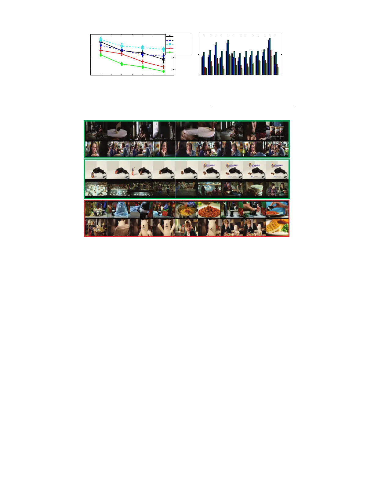
1 Rob ust Subjectiv e Visual Proper ty Prediction from Cro wdsourced P airwise Labels Y anwei Fu, Timoth y M. Hospedales, T ao Xiang, Jiechao Xiong, Shaogang Gong, Yizhou W ang, and Y uan Y ao Abstract —The problem of estimating subjectiv e visual proper ties from image and video has attracted increasing interest. A subjectiv e visual proper ty is useful either on its own (e.g. image and video interestingness) or as an intermediate representation f or visual recognition (e.g. a relativ e attr ibute). Due to its ambiguous nature , annotating the value of a subjectiv e visual proper ty for learning a prediction model is challenging. T o make the annotation more reliable , recent studies employ crowdsourcing tools to collect pairwise comparison labels. Howe ver , using crowdsourced data also introduces outliers. Existing methods rely on majority v oting to prune the annotation outliers/errors. The y thus require a large amount of pairwise labels to be collected. More importantly as a local outlier detection method, major ity voting is ineffectiv e in identifying outliers that can cause global ranking inconsistencies . In this paper , we propose a more principled w ay to identify annotation outliers by formulating the subjective visual property prediction task as a unified robust lear ning to rank prob lem, tackling both the outlier detection and learning to rank jointly . This differs from e xisting methods in that (1) the proposed method integrates local pairwise compar ison labels together to minimise a cost that corresponds to global inconsistency of ranking order , and (2) the outlier detection and learning to ran k problems are solved jointly . This not only leads to better detection of annotation outliers but also enab les lear ning with extremely sparse annotations . Index T erms —Subjective visual proper ties, outlier detection, rob ust ranking, robust learning to rank, regularisation path F 1 I N T RO D U C T I O N The solutions to many computer vision problems involve the estimation of some visual properties of an image or video, r epresented as either discr ete or continuous vari- ables. For example scene classification aims to estimate the value of a discrete variable indicating which scene category an image belongs to; for object detection the task is to estimate a binary variable corresponding the presence/absence of the object of inter est and a set of variables indicating its whereabouts in the image plane (e.g. four variables if the whereabouts are repr esented as bounding boxes).Most of these visual properties ar e objective; that is, there is no or little ambiguity in their true values to a human annotator . In comparison, the pr oblem of estimating subjective visual properties is much less studied. This class of computer vision problems nevertheless encompass a va- riety of important applications. For example: estimating attractiveness [1] from faces would inter est social media or online dating websites; and estimating properties of consumer goods such as shininess of shoes [2] improves • Y anwei Fu, T imothy M. Hospedales, T ao Xiang, and Shaogang Gong are with the School of Electronic Engineering and Computer Sci- ence, Queen Mary University of London, E1 4NS, UK. Email: {y.fu, t.hospedales,t.xiang,s.gong}@qmul.ac.uk. • Jiechao Xiong, and Y uan Y ao are with the School of Mathematical Sciences, Peking University, China. Email: xiongjiechao@pku.edu.cn, yuany@math.pku.edu.cn. Y izhou Wang is with Nat’l Engineering Lab- oratory for V ideo T echnology Cooperative Medianet Innovation Center Key Laboratory of Machine Perception (MoE) Sch’l of EECS, Peking University , Beijing, 100871, China. Email: yizhou.wang@pku.edu.cn. customer experiences on online shopping websites. Re- cently , the problem of automatically pr edicting if people would find an image or video interesting has started to receive increasing attention [3], [4], [5]. Inter estingness prediction has a number of real-world applications. In particular , since the number of images and videos up- loaded to the Internet is growing explosively , people are increasingly relying on image/video recommendation tools to select which ones to view . Given a query , ranking the retrieved data with relevance to the query based on the predicted interestingness would improve user satisfaction. Similarly user stickiness can be increased if a media-sharing website such as Y ouT ube can rec- ommend videos that are both relevant and interesting. Other applications such as web advertising and video summarisation can also benefit. Subjective visual prop- erties such as the above-mentioned ones are useful on their own. But they can also be used as an intermediate repr esentation for other tasks such as visual recognition, e.g., differ ent people can be recognised by how pale their skin complexions are and how chubby their faces are [6]. When used as a semantically meaningful r epresentation, these subjective visual properties often are r eferred to as relative attributes [2], [6], [7]. Learning a model for subjective visual property (SVP) prediction is challenging primarily due to the difficulties in obtaining annotated training data. Specifically , since most SVPs can be repr esented as continuous variables (e.g. an inter estingness/aesthetics/shininess score with a value range of 0 to 1 with 1 being most interest- ing/aesthetically appealing/shinning), SVP prediction can be cast as a regression problem – the low-level 2 feature values are regressed to the SVP values given a set of training data annotated with their true SVP values. However , since by definition these properties are subjective, differ ent human annotators often struggle to give an absolute value and as a result the annotations of differ ent people on the same instance can vary hugely . For example, on a scale of 1 to 10, differ ent people will have very different ideas on what a scale 5 means for an image, especially without any common reference point. On the other hand, it is noted that humans can in general more accurately rank a pair of data points in terms of their visual properties [8], [9] , e.g. it is easier to judge which of two images is more inter esting relatively than giving an absolute interestingness scor e to each of them. Most existing studies [2], [1], [9] on SVP prediction thus take a learning to rank approach [10], where annotators give comparative labels about pairs of images/videos and the learned model is a ranking function that predicts the SVP value as a ranking score. T o annotate these pairwise comparisons, crowdsour c- ing tools such as Amazon Mechanic T urk (AMT) are resorted to, which allow a large number of annotators to collaborate at very low cost. Data annotation based on cr owdsourcing is incr easingly popular [6], [2], [4], [5] recently for annotating large-scale datasets. However , this brings about two new problems: (1) Outliers – The crowd is not all trustworthy: it is well known that crowdsour ced data are greatly affected by noise and out- liers [11], [12], [13] which can be caused by a number of factors. Some workers may be lazy or malicious [14], pro- viding random or wrong annotations either carelessly or intentionally; some other outliers are unintentional hu- man errors caused by the ambiguous nature of the data, thus ar e unavoidable r egardless how good the attitudes of the workers are. For example, the pairwise ranking for Figur e 1(a) depends on the cultural/psychological background of the annotator – whether s/he is more familiar/prefers the story of Monkey King or Cookie Monster 1 . When we learn the model fr om labels collected from many people, we essentially aim to learn the con- sensus, i.e. what most people would agree on. Therefore, if most of the annotators growing up watching Sesame Street thus consciously or subconsciously consider the Cookie Monster to be mor e interesting than the Monkey King, their pairwise labels/votes would repr esent the consensus. In contrast, one annotator who is familiar with the stories in Journey to the W est may choose the opposite; his/her label is thus an outlier under the consensus. (2) Sparsity – the number of pairwise comparisons requir ed is much bigger than the number of data points because n instances define a O ( n 2 ) pairwise space. Consequently , even with crowdsour cing tools, the annotation remains be sparse, i.e. not all pairs ar e compared and each pair is only compared a few times. T o deal with the outlier problem in crowdsour ced data, existing studies take a majority voting strategy [6], 1. This is also known as Halo Effect in Psychology . ? ? Who is smiling more? Who is more interesting? (a) (b) Figure 1. Examples of pairwise compar isons of subjective visual proper ties. [2], [4], [15], [16], [17], [18]. That is, a large budget of 5 − 10 times the number of actual annotated pairs requir ed is allocated to obtain multiple annotations for each pair . These annotations are then averaged over so as to eliminate label noise. However , the effectiveness of the majority voting strategy is often limited by the sparsity problem – it is typically infeasible to have many annota- tors for each pair . Furthermore, there is no guarantee that outliers, particularly those caused by unintentional hu- man err ors can be dealt with effectively . This is because majority voting is a local consistency detection based strategy – when there are contradictory/inconsistent pairwise rankings for a given pair , the pairwise rankings receiving minority votes ar e eliminated as outliers. How- ever , it has been found that when pairwise local rankings are integrated into a global ranking, it is possible to detect outliers that can cause global inconsistency and yet ar e locally consistent, i.e. supported by majority votes [19]. Critically , outliers that cause global inconsistency have more significant detrimental effects on learning a ranking function for SVP prediction and thus should be the main focus of an outlier detection method. In this paper we propose a novel approach to sub- jective visual property prediction from sparse and noisy pairwise comparison labels collected using crowdsour c- ing tools. Dif ferent from existing approaches which first remove outliers by majority voting, followed by r egres- sion [4] or learning to rank [5], we formulate a unified r o- bust learning to rank (URLR) framework to solve jointly both the outlier detection and learning to rank problems. Critically , instead of detecting outliers locally and inde- pendently at each pair by majority voting, our outlier detection method operates globally , integrating all local pairwise comparisons together to minimise a cost that corresponds to global inconsistency of ranking order . This enables us to identify those outliers that receive majority votes but cause large global ranking inconsis- tency and thus should be removed. Furthermor e, as a global method that aggregates comparisons across dif- ferent pairs, our method can operate with as few as one comparison per pair , making our method much more robust against the data sparsity pr oblem compared to the conventional majority voting appr oach that aggregates comparisons for each pair in isolation. More specifically , the proposed model generalises a partially penalised LASSO optimisation or Huber-LASSO formulation [20], 3 [21], [22] from a robust statistical ranking formulation to a robust learning to rank model, making it suitable for SVP prediction given unseen images/videos. W e also formulate a regularisation path based solution to solve this new formulation efficiently . Extensive experiments are carried out on benchmark datasets including two image and video interestingness datasets [4], [5] and two relative attribute datasets [2]. The r esults demonstrate that our method significantly outperforms the state-of- the-art alternatives. 2 R E L A T E D W O R K Subjective visual properties Subjective visual prop- erty pr ediction covers a lar ge variety of computer vision problems; it is thus beyond the scope of this paper to present an exhaustive review here. Instead we focus mainly on the image/video interestingness prediction problem which share many characteristics with other SVP prediction problem such as image quality [23], memorability [24], and aesthetics [3] prediction. Predicting image and video interestingness Early ef- forts on image inter estingness prediction focus on dif- ferent aspects than interestingness as such, including memorability [24] and aesthetics [3]. These SVPs are related to interestingness but dif ferent. For instance, it is found that memorability can have a low correlation with interestingness - people often remember things that they find uninteresting [4]. The work of Gygli et al [4] is the first systematic study of image interestingness. It shows that three cues contribute the most to inter estingness: aesthetics, unusualness/novelty and general pr eferences, the last of which refers to the fact that people in general find certain types of scenes more interesting than oth- ers, for example outdoor-natural vs. indoor -manmade. Differ ent featur es ar e then designed to repr esent these cues as input to a prediction model. In comparison, video interestingness has r eceived much less attention, per haps because it is even har der to understand its meaning and contributing cues. Liu et al. [25] focus on key frames so essentially treats it as an image interestingness problem, whilst [5] is the first work that proposes benchmark video interestingness datasets and evaluates differ ent features for video interestingness pr ediction. Most earlier works cast the aesthetics or inter esting- ness prediction pr oblem as a regr ession problem [23], [3], [24], [25]. However , as discussed before, obtaining an ab- solute value of interestingness for each data point is too subjective and affected too much by unknown personal prefer ence/social background to be reliable. Therefor e the most recent two studies on image [4] and video [5] interestingness all collect pairwise comparison data by crowdsourcing. Both use majority voting to r emove outliers first. After that the prediction models differ – [4] converts pairwise comparisons into an absolute interestingness values and use a regression model, whilst [5] employs rankSVM [10] to learn a ranking function, with the estimated ranking score of an unseen video used as the interestingness prediction. W e compare with both approaches in our experiments and demonstrate that our unified robust learning to rank approach is superior as we can remove outliers mor e effectively – even if they correspond to comparisons receiving major- ity votes, thanks to its global formulation. Relative attributes In a broader sense interestingness can be considered as one type of relative attribute [6]. Attribute-based modelling [26], [27] has gained popu- larity recently as a way to describe instances and classes at an intermediate level of r epresentation. Attributes are then used for various tasks including N-shot and zero- shot transfer learning. Most previous studies consider binary attributes [26], [27]. Relative attributes [6] were recently proposed to learn a ranking function to predict relative semantic strength of visual attributes. Instead of the original class-level attribute comparisons in [6], this paper focuses on instance-level comparisons due to the huge intra-class variations in r eal-world problems. W ith instance-level pairwise comparisons, r elative attributes have been used for interactive image search [2], and semi-supervised [28] or active learning [29], [30] of visual categories. However , no previous work addresses the problem of annotation outliers except [2], which adopts the heuristic majority voting strategy . Learning from noisy paired crowdsourced data Many large-scale computer vision problems rely on human intelligence tasks (HIT) using crowdsour cing services, e.g. AMT (Amazon Mechanical T urk) to collect an- notations. Many studies [14], [31], [32], [13] highlight the necessity of validating the random or malicious labels/workers and give filtering heuristics for data cleaning. However , these ar e primarily based on majority voting which requir es a costly volume of redundant annotations, and has no theoretical guarantee of solving the outlier and sparsity problems. As a local (per-pair) filtering method, majority voting does not r espect global ordering and even risks introducing additional incon- sistency due to the well-known Condorcet’s paradox in social choice and voting theory [33]. Active learning [34], [29], [30] is an another way to circumvent the O ( n 2 ) pair - wise labelling space. It actively poses specific requests to annotators and learns from their feedback, rather than the ‘general’ pairwise comparisons discussed in this work. Besides paired crowdsour ced data, majority vot- ing is more widely used in crowdsourcing where mul- tiple annotators directly label instances, which attracted lots of attention in the machine learning community [16], [17], [18], [15]. In contrast, our work focuses on pairwise comparisons which are relatively easier for annotators in evaluating the subjective visual pr operties [8] . Statistical ranking and learning to rank Statistical rank- ing has been widely studied in statistics and computer science [35], [36], [8], [37]. However , statistical ranking only concerns the ranking of the observed/training data, but not learning to predict unseen data by learning ranking functions. T o learn ranking functions for ap- plications such as interestingness prediction, a feature 4 repr esentation of the data points must be used as model input in addition to the local ranking orders. This is addressed in learning to rank which is widely studied in machine learning [38], [39], [40]. However , existing learning to rank works do not explicitly model and remove outliers for r obust learning: a critical issue for learning from crowdsour ced data in practice. In this work, for the first time, we study the problem of ro- bust learning to rank given extremely noisy and sparse crowdsour ced pairwise labels. W e show both theoreti- cally and experimentally that by solving both the outlier detection and ranking prediction problems jointly , we achieve better outlier detection than existing statistical ranking methods and better ranking prediction than existing learning to rank method such as RankSVM without outlier detection. Our contributions are threefold: (1) W e propose a novel robust learning to rank method for subjective visual property prediction using noisy and sparse pairwise comparison/ranking labels as training data. (2) For the first time, the problems of detecting outliers and estimat- ing linear ranking models are solved jointly in a unified framework. (3) W e demonstrate both theor etically and experimentally that our method is superior to existing majority voting based methods as well as statistical rank- ing based methods. An earlier and preliminary version of this work is presented in [41] which focused only on the image/video inter estingness prediction pr oblem. 3 U N I FI E D R O B U S T L E A R N I N G T O R A N K 3.1 Problem definition W e aim to learn a subjective visual property (SVP) prediction model from a set of sparse and noisy pairwise comparison labels, each comparison corresponding to a local ranking between a pair of images or videos. Suppose our training set has N data points/instances repr esented by a feature matrix Φ = h φ T i i N i =1 ∈ R N × d , where φ i is a d -dimensional column low-level featur e vector representing instance i . The pairwise comparison labels (annotations collected using crowdsour cing tools) can be naturally r epresented as a dir ected comparison graph G = ( V , E ) with a node set V = { i } N i =1 corre- sponding to the N instances and an edge set E = { e ij } corresponding to the pairwise comparisons. The pairwise comparison labels can be provided by multiple annotators. They are dichotomously saved: Suppose annotator α gives a pairwise comparison for instance i and j ( i, j ∈ V ). If α considers that the SVP of instance i is stronger/mor e than that of j , we save ( i, j, y α e ij ) and set y α e ij = 1 . If the opposite is the case, we save ( j, i, y α e j i ) and set y α e j i = 1 . All the pairwise comparisons between instances i and j ar e then aggre- gated over all annotators who have cast a vote on this pair; the results are repr esented as w e ij = P α J y α e ij = 1 K which is the total number of votes on i over j for a specific SVP , where JK indicates the Iverson’s bracket notation, and w e j i which is defined similarly . This gives an edge weight vector w =  w e ij  ∈ R | E | where | E | is the number of edges. Now the edge set can be represented as E =  e ij | w e ij > 0  and w e ij ∈ R is the weight for the edge e ij . In other words, an edge e ij : i → j exists if w e ij > 0 . The topology of the graph is denoted by a flag indicator vector y =  y e ij  ∈ R | E | where each indicator y e ij = 1 indicates that there is an edge between instances i to j regar dless how many votes it carries. Note that all the elements in y have the value 1 , and their index e ij gives the corr esponding nodes in the graph. Given the training data consisting of the feature matrix Φ and the annotation graph G , there are two tasks: 1) Detecting and r emoving the outliers in the edge set E of G . T o this end, we introduce a set of unknown variables γ =  γ e ij  ∈ R | E | where each variable γ e ij indicates whether the edge e ij is an outlier . The outlier detection problem thus becomes the problem of estimating γ . 2) Estimating a prediction function for SVP . In this work a linear model is considered due to its low computational complexity , that is, given the low- level feature φ x of a test instance x we use a linear function f ( x ) = β T φ x to pr edict its SVP , where β is the coef ficient weight vector of the low-level feature φ x . Note that all formulations can be easily updated to use a non-linear function. So far in the introduced notations three vectors shar e indices: the flag indicator vector y , the outlier variable vector γ and the edge weight vector w . For notation convenience, from now on we use y ij , γ ij and w ij to replace y e ij , γ e ij and w e ij respectively . As in most graph based model formulations, we define C ∈ R | E |× N as the incident matrix of the directed graph G , where C e ij i = − 1 / 1 if the edge e ij enters/leaves vertex i . Note that in an ideal case, one hopes that the votes received on each pair are unanimous, e.g. w ij > 0 and w j i = 0 ; but often there ar e disagreements, i.e. we have both w ij > 0 and w j i > 0 . Assuming both cannot be true simultaneously , one of them will be an outlier . In this case, one is the majority and the other minority which will be pruned by the majority voting method. This is why majority voting is a local outlier detection method and requires as many votes per pair as possible to be effective (the wisdom of a crowd). 3.2 Framew ork formulation In contrast to majority voting, we propose to prune outliers globally and jointly with learning the SVP pre- diction function. T o this end, the outlier variables γ ij for outlier detection and the coef ficient weight vector β for SVP prediction are estimated in a unified framework. Specifically , for each edge e ij ∈ E , its corresponding flag indicator y ij is modelled as y ij = β T φ i − β T φ j + γ ij + ε ij , (1) where ε ij ∼ N (0 , σ 2 ) is the Gaussian noise with zero mean and a variance σ , and the outlier variable γ ij ∈ R 5 is assumed to have a higher magnitude than σ . For an edge e ij , if y ij is not an outlier , we expect β T φ i − β T φ j should be approximately equal to y ij , therefor e we have γ ij = 0 . On the contrary , when the pr ediction of β T φ i − β T φ j differs greatly from y ij , we can explain y ij as an outlier and compensate for the discrepancy between the prediction and the annotation with a nonzero value of γ ij . The only prior knowledge we have on γ ij is that it is a sparse variable, i.e. in most cases γ ij = 0 . For the whole training set, Eq (1) can be re-written in its matrix form y = C Φ β + γ +  (2) where y = [ y ij ] ∈ R | E | , γ = [ γ ij ] ∈ R | E | ,  = [ ε ij ] ∈ R | E | and C ∈ R | E |× N is the incident matrix of the annotation graph G . In order to estimate the | E | + d unknown parameters ( | E | for γ and d for β ), we aim to minimise the dis- crepancy between the annotation y and our prediction C Φ β + γ , as well as keeping the outlier estimation γ sparse. Note that y only contains information about which pairs of instances have r eceived votes, but not how many . The discrepancy thus needs to weighted by the number of votes received, repr esented by the edge weight vector w = [ w ij ] ∈ R | E | . T o that end, we put a weighted l 2 − loss on the discr epancy and a sparsity enhancing penalty on the outlier variables. This gives us the following cost function: L ( β , γ ) = 1 2 k y − C Φ β − γ k 2 2 , w + p λ ( γ ) (3) where k y − C Φ β − γ k 2 2 , w = X e ij ∈ E w ij ( y ij − γ ij − β T φ i + β T φ j ) 2 , and p λ ( γ ) is the sparsity constraint on γ . W ith this cost function, our Unified Robust Learning to Rank (URLR) framework identifies outliers globally by integrating all local pairwise comparisons together . Note that in Eq (3), the noise term  has been removed because the discrepancy is mainly caused by outliers due to their larger magnitude. Ideally the sparsity enhancing penalty term p λ ( γ ) should be a l 0 regularisation term. However , for a tractable solution, a l 1 regularisation term is used: p λ ( γ ) = λ k γ k 1 , w = λ P e ij w ij | γ ij | , where λ is a free parameter corr esponding to the weight for the r egulari- sation term. W ith this l 1 penalty term, the cost function becomes convex: L ( β , γ ) = 1 2 k √ W ( y − γ ) − X β k 2 2 + λ k γ k 1 , w , (4) where X = √ W C Φ , W = diag( w ) is the diagonal matrix of w and √ W = diag( √ w ) . Setting ∂ L ∂ β = 0 , the problem of minimisation of the cost function in (4) can be decomposed into the following two subproblems: 1) Estimating the parameters β of the prediction func- tion f ( x ) : ˆ β = ( X T X ) † X T √ W ( y − γ ) , (5) Mathematically , the Moore-Penr ose pseudo- inverse of X T X is defined as ( X T X ) † = lim µ → 0 (( X T X ) T ( X T X ) + µI ) − 1 ( X T X ) T , where I is the identity matrix. The scalar variable µ is introduced to avoid numerical instability [42], and typically assumes a small value 2 . W ith the the introduction of µ , Eq (5) becomes: ˆ β = ( X T X + µI ) − 1 X T √ W ( y − γ ) . (6) A standard solver for Eq (6) has a O ( | E | d 2 ) com- putational complexity , which is almost linear with respect to the size of the graph | E | if d  n . Faster algorithms based on the Krylov iterative and algebraic multi-grid methods [43] can also be used. 2) Outlier detection: ˆ γ = ar g min γ 1 2 k ( I − H ) √ W ( y − γ ) k 2 2 + λ k γ k 1 , w (7) = arg min γ 1 2 k ˜ y − e X γ ) k 2 2 + λ k γ k 1 , w (8) where H = X ( X T X ) † X T is the hat matrix, e X = ( I − H ) √ W and ˜ y = ˜ X y . Eq (7) is obtained by plugging the solution ˆ β back into Eq (4). 3.3 Outlier detection by regularisation path From the formulations described above, it is clear that outlier detection by solving Eq (8) is the key – once the outliers ar e identified, the estimated ˆ γ can be used to substitute γ in Eq (5) and the estimation of the prediction function parameter β becomes straightforward. Now let us focus on solving Eq (8) for outlier detection. Note that solving Eq (8) is essentially a LASSO (Least Absolute Shrinkage and Selection Operator) [20] prob- lem. For a LASSO problem, tuning the regularisation parameter λ is notoriously dif ficult [44], [45], [46], [47]. In particular , in our URLR framework, the λ value dir ectly decides the ratio of outliers in the training set which is unknown. A number of methods for determining λ exist, but none is suitable for our formulation: 1) Some heuristics rules on setting the value of λ such as λ = 2 . 5 ˆ σ are popular in existing robust ranking models such as the M-estimator [44], where ˆ σ is a Gaussian variance set manually based on human prior knowledge. However setting a constant λ value independent of dataset is far fr om optimal because the ratio of outliers may vary for dif ferent crowdsour ced datasets. 2) Cross validation is also not applicable her e because each edge e ij is associated with a γ ij variable and any held-out edge e ij also has an associated unknown variable γ ij . As a result, cross validation can only optimise part of the sparse variables while 2. In this work, µ is set to 0 . 001 . 6 leaving those for the held-out validation set unde- termined. 3) Data adaptive techniques such as Scaled LASSO [45] and Square-Root LASSO [46] typically generate over-estimates on the support set of outliers. More- over , they rely on the homogeneous Gaussian noise assumption which is often not valid in practice. 4) The other alternatives e.g. Akaike information cri- terion (AIC) and Bayesian information criterion (BIC) are often unstable in outlier detection LASSO problems [47] 3 . This inspires us to sequentially consider all available solutions for all sparse variables along the Regularisation Path (RP) by gradually decreasing the value of the regularisation parameter λ from ∞ to 0 . Specifically , based on the piecewise-linearity pr operty of LASSO, a regularisation path can be efficiently computed by the R- package “glmnet" [48] 4 . When λ = ∞ , the regularisation parameter will str ongly penalise outlier detection: if any annotation is taken as an outlier , it will greatly incr ease the value of the cost function in Eq (8). When λ is changed from ∞ to 0 , LASSO 5 will first select the vari- able subset accounting for the highest deviations to the observations e X in Eq (8). These high deviations should be assigned higher priority to represent the nonzero elements 6 of γ of Eq (2), because γ compensates the discrepancy between annotation and prediction. Based on this idea, we can order the edge set E according to which nonzero γ ij appears first when λ is decreased from ∞ to 0 . In other words, if an edge e ij whose associated outlier variable γ ij becomes nonzero at a larger λ value, it has a higher probability to be an outlier . Following this or der , we identify the top p % edge set Λ p as the annotation outliers. And its complementary set Λ 1 − p = E \ Λ p are the inliers. Therefor e, the outcome of estimating γ using Eq (8) is a binary outlier indicator vector f =  f e ij  : f e ij = ( 1 e ij ∈ Λ 1 − p 0 e ij ∈ Λ p where each element f e ij indicates whether the corre- sponding edge e ij is an outlier or not. Now with the outlier indicator vector f estimated using regularisation path, instead of estimating β by substituting γ in Eq (5) with an estimated ˆ γ , β can be computed as ˆ β = ( X T F X + µI ) − 1 X T √ W F y (9) 3. W e found empirically that the model automatically selected by BIC or AIC failed to detect any meaningful outliers in our experi- ments. For details of the experiments and a discussion on the issue of determining the outlier ratio, please visit the project webpage at http://www .eecs.qmul.ac.uk/~yf300/ranking/index.html 4. http://cran.r- project.org/web/packages/glmnet/glmnet.pdf 5. For a thorough discussion from a statistical perspective, please see [49], [50], [51], [47]. 6. This is related with LASSO for covariate selection in a graph. Please see [52] for more details. Algorithm 1 Learning a unified robust learning to rank (URLR) model for SVP pr ediction Input : A training dataset consisting of the feature matrix Φ and the pairwise annotation graph G , and an outlier pruning rate p % . Output : Detected outliers f and prediction model pa- rameter β . 1) Solve Eq (8) using Regularisation Path; 2) T ake the top p % pairs as outliers to obtain the outlier indicator vector f ; 3) Compute β using Eq (9). where F = diag ( f ) , that is, we use f to ‘clean up’ y before estimating β . The pseudo-code of learning our URLR model is sum- marised in Algorithm 1. 3.4 Discussions 3.4.1 Advantage ov er major ity voting The proposed URLR framework identifies outliers glob- ally by integrating all local pairwise comparisons to- gether , in contrast to the local aggr egation based majority voting. Figur e 2(a) illustrates why our URLR framework is advantageous over the local majority voting method for outlier detection. Assume ther e are five images A − E with five pairs of them compared thr ee times each, and the correct global ranking order of these 5 images in terms of a specific SVP is A < B < C < D < E . Figure 2(a) shows that among the five compared pairs, majority voting can successfully identify four outlier cases: A > B , B > C , C > D , and D > E , but not the fifth one E < A . However when considered globally , it is clear that E < A is an outlier because if we have A < B < C < D < E , we can deduce A < E . Our formulation can detect this tricky outlier . Mor e specifi- cally , if the estimated β makes β T φ A − β T φ E > 0 , it has a small local inconsistency cost for that minority vote edge A → E . However , such β value will be ‘propagated’ to other images by using the voting edges B → A , C → B , D → C , and E → D , which ar e accumulated into a much bigger global inconsistency with the annotation. This enables our model to detect E → A as an outlier , contrary to the majority voting decision. In particular , the majority voting will introduce a loop comparison A < B < C < D < E < A which is the well-known Condorcet’s paradox [33], [19]. W e further give two more extr eme cases in Figur es 2(b) and (c). Due to the Condorcet’s paradox, in Figure 2(b) the estimated β from majority voting, which removes A → E , is even worse than that from all annotation pairs which at least save the correct annotation A → E . Furthermore, Figur e 2(c) shows that when each pair only receives votes in one dir ection, majority voting will cease to work altogether , but our URLR can still detect outliers by examining the global cost. This example thus high- lights the capability of URLR in coping with extremely 7 2 1 2 1 2 1 2 1 2 1 D E C B A (a) 2 1 2 2 2 2 D E C B A (b) 2 2 1 2 2 D E C B A (c) Figure 2. Better outlier detection can be achiev ed using our URLR frame work than major ity voting. Green ar- rows/edges indicate correct annotations, while red arrows are outliers. The numbers indicate the number of votes received b y each edge. sparse pairwise comparison labels. In our experiments (see Section 4), the advantage of URLR over majority is validated on various SVP pr ediction problems. 3.4.2 Advantage ov er robust statistical ranking Our framework is closely related to Huber ’s theory of robust regression [44], which has been used for robust statistical ranking [53]. In contrast to learning to rank, robust statistical ranking is only concerned with ranking a set of training instances by integrating their (noisy) pairwise rankings. No low-level feature repr esentation of the instances is used as robust ranking does not aim to learn a ranking pr ediction function that can be applied to unseen test data. T o see the connection between URLR with robust ranking, consider the Huber M-estimator [44] which aims to estimate the optimal global ranking for a set of training instances by minimising the follow- ing cost function: min θ X i,j w ij ρ λ (( θ i − θ j ) − y ij ) (10) where θ = [ θ i ] ∈ R | E | is the ranking score vector storing the global ranking score of each training instance i . The Huber ’s loss function ρ λ ( x ) is defined as ρ λ ( x ) =  x 2 / 2 , if | x | ≤ λ λ | x | − λ 2 / 2 , if | x | > λ . (11) Using this loss function, when | ( θ i − θ j ) − y ij | < λ , the comparison is taken as a “good” one and penalised by an l 2 − loss for Gaussian noise. Otherwise, it is regarded as a sparse outlier and penalised by an l 1 − loss. It can be shown [53] that robust ranking with Huber ’s loss is equivalent to a LASSO problem, which can been applied to joint r obust ranking and outlier detection [47]. Specif- ically , the global ranking of the training instances and the outliers in the pairwise rankings can be estimated as n ˆ θ , ˆ γ o = min θ , γ 1 2 k y − C θ − γ k 2 2 , w + λ k γ k 1 , w (12) = min θ , γ X e ij ∈ E w ij  k 1 2 ( y ij − γ ij − ( θ i − θ j ) k 2 + λ | γ ij |  (13) The optimisation problem (12) is designed for solving the robust ranking pr oblem with Huber ’s loss function, hence called Huber -LASSO [53]. Our URLR can be considered as a generalisation of the Huber-LASSO based r obust ranking pr oblem above. Comparing Eq (12) with Eq (3), it can be seen that the main differ ence between URLR and conventional robust ranking is that in URLR the cost function has the low-level feature matrix Φ computed from the training instances, and the prediction function parameter β , such that θ = Φ β . This is because the objective of URLR is to predict SVP for unseen test data. However , URLR and robust ranking do share one thing in common – the ability to detect outliers in the training data based on a Huber-LASSO formulation. This means that, as opposed to our unified framework with feature Φ , one could design a two-step approach for learning to rank by first identifying and removing outliers using Eq (12), followed by introducing the low-level feature matrix Φ and prediction model parameter β and estimating β using Eq (9). W e call this approach Huber-LASSO-FL based learning to rank which dif fers from URLR mainly in the way outliers are detected without considering low level features. Next we show that there is a critical theoretical ad- vantage of URLR over conventional Huber-LASSO in detecting outliers from the training instances. This is due to the dif ference in the pr ojection space for estimating γ which is denoted as Γ . T o explain this point, we decompose X in Eq (8) by Singular V alue Decomposition (SVD), X = U Σ V T (14) where U = [ U 1 , U 2 ] with U 1 being an orthogonal basis of the column space of X and U 2 an orthogonal basis of its complement. Therefore, due to the orthogonality U T U = I and U T 2 X = 0 , we can simplify Eq (8) into ˆ γ = arg min γ kU T 2 y − U T 2 γ k 2 2 , w + λ k γ k 1 , w . (15) The SVD orthogonally projects y onto the column space of X and its complement, while U 1 is an orthogo- nal basis of the column space X and U 2 is the orthogonal basis of its complement Γ (i.e. the kernel space of X T ). W ith the SVD, we can now compute the outliers ˆ γ by solving Eq (15) which again is a LASSO problem [42], where outliers provide sparse approximations of projection U T 2 y . W e can thus compare dimensions of the projection spaces of URLR and Huber-LASSO-FL: • Robust ranking based on the featureless Huber- LASSO-FL 7 : to see the dimension of the projection space Γ , i.e. the space of cyclic rankings [19], [53], we can perform a similar SVD operation and r ewrite Eq (12) in the same form as Eq (15), but this time we have X = √ W C , U 1 ∈ R | E |× ( | V |− 1) and U 2 ∈ R | E |× ( | E |−| V | +1) . So the dimension of Γ for Huber- LASSO-FL is dim(Γ) = | E | − | V | + 1 . • URLR: in contrast we have X = √ W C Φ , U 1 ∈ R | E |× d and U 2 ∈ R | E |× ( | E |− d ) . So the dimension of Γ for URLR is dim(Γ) = | E | − d . 7. W e assume that the graph is connected, that is, | E | ≥ | V | − 1 ; we thus have rank( C ) = | V | − 1 . 8 From the above analysis we can see that given a very sparse graph with | E | ∼ | V | , the pr ojection space Γ for Huber-LASSO-FL will have a dimension ( | E | − | V | + 1 ) too small to be ef fective for detecting outliers. In contrast, by exploiting a low dimensional ( d  | V | ) feature repr esentation of the original node space, URLR can enlarge the projection space to that of dimension | E | − d . Our URLR is thus able to enlarges its outlier detection projection space Γ . As a result our URLR can better identify outliers, especially for sparse pairwise anno- tation graphs. In general, this advantage exists when the feature dimension d is smaller than the number of training instance | V | = N , and the smaller the value of d , the bigger the advantage over Huber-LASSO. In practice, given a large training set we typically have d  | V | . On the other hand, when the number of instances is small, and each instance is r epresented by a high-dimensional feature vector , we can always reduce the feature dimension using techniques such as PCA to make sure that d  | V | . This theoretical advantage of URLR over conventional Huber -LASSO in outlier detection is validated experimentally in Section 4. 3.4.3 Regularisation on β It is worth mentioning that in the cost function of URLR (Eq (3)), there are two sets of variables to be estimated, γ and β , but only one l 1 regularisation term on γ to enforce sparsity . When the dimensionality of β (i.e. d ) is high, one would expect to see a l 2 regularisation term on β (e.g. ridge regression) due to the fact that the coefficients of highly correlated low-level features can be poorly estimated and exhibit high variance without imposing a proper size constraint on the coefficients [42]. The reason we do not include such a regularisation term is because, as mentioned above, using URLR we need to make sure the low-level feature space dimensionality d is low , which means that the dimensionality of β is also low , making the regularisation term β redundant. This leads to the applicability of much simpler solvers and we show empirically in the next section that satisfactory results can be obtained with this simplification. 4 E X P E R I M E N T S Experiments were carried out on five benchmark datasets (see T able 1) which fall into thr ee categories: (1) experiments on estimating subjective visual properties (SVPs) that are useful on their own including image (Section 4.1) and video interestingness (Section 4.2), (2) experiments on estimating SVPs as relative attributes for visual recognition (Section 4.3), and (3) experiments on human age estimation from face images (Section 4.4). The third set of experiments can be considered as synthetic experiments – human age is not a subjective visual property although it is ambiguous and poses a problem even for humans [56]. However , as gr ound truth is available, this set of experiments ar e designed to gain insights into how dif ferent SVP prediction models work. 4.1 Image interestingness prediction Datasets The image inter estingness dataset was first introduced in [24] for studying memorability . It was later re-annotated as an image interestingness dataset by [4]. It consists of 2222 images. Each was repr esented as a 915 dimensional attribute 8 feature vector [24], [4] such as central object, unusual scene and so on. 16000 pairwise comparisons were collected by [4] using AMT and used as annotation. On average, each image is viewed and compared with 11.9 other images, resulting a total of 16000 pairwise labels 9 . Settings 1000 images were randomly selected for training and the remaining 1222 for testing. All the ex- periments were repeated 10 times with different random training/test splits to reduce variance. The pruning rate p was set to 20% . W e also varied the number of annotated pairs used to test how well each compar ed method copes with increasing annotation sparsity . Evaluation metrics For both image and video inter - estingness prediction, Kendall tau rank distance was employed to measure the percentage of pairwise mis- matches between the predicted ranking order for each pair of test data using their pr ediction/ranking function scores, and the gr ound truth ranking pr ovided by [4] and [5] respectively . Larger Kendall tau rank distance means lower quality of the ranking order predicted. Competitors W e compare our method (URLR) with four competitors. 1) Maj-V ot-1 [5]: this method uses majority voting for outlier pruning and rankSVM for learning to rank. 2) Maj-V ot-2 [4]: this method also first removes out- liers by majority voting. After that, the fraction of selections by the pairwise comparisons for each data point is used as an absolute interestingness score and a regr ession model is then learned for prediction. Note that Maj-V ot-2 was only compared in the experiments on image and video interesting- ness prediction, since only these two datasets have enough dense annotations for Maj-V ot-2 . 3) Huber-LASSO-FL : robust statistical ranking that performs outlier detection using the conventional featureless Huber -LASSO as described in Section 3.4.2, followed by estimating β using Eq (9). 4) Raw : our URLR model without outlier detection, that is, all annotations ar e used to estimate β . Comparative results The interestingness prediction performance of the various models are evaluated while varying the amount of pairwise annotation used. The results are shown in Figure 3 (left). It shows clearly that our URLR significantly outperforms the four alternatives for a wide range of annotation density . This validates the effectiveness of our method. In particular , it can 8. W e delete 8 attribute features from the original feature vector in [24], [4] such as “attractive” because they are highly corr elated with image interestingness. 9. On average, for each labelled pair , around 80% of the annotations agree with one ranking order and 20% the other . 9 Dataset No. pairs No. img/video Feature Dim. No. classes Image Interestingness [24] 16000 2222 932 (150) 1 V ideo Interestingness [5] 60000 420 1000 (60) 14 PubFig [54], [2] 2616 772 557 (100) 8 Scene [55], [2] 1378 2688 512 (100) 8 FG-Net Face Age Dataset [56] – 1002 55 – T ab le 1 Dataset summar y . We use the original f eatures to lear n the ranking model (Eq (9)) and reduce the f eature dimension (values in brac kets) using K er nel PCA [57] to improve outlier detection (Eq (8)) b y enlarging the projection space of γ . 30 40 50 60 70 80 90 100 110 0.11 0.12 0.13 0.14 0.15 0.16 0.17 Percentage of total available pairs (%) Kendall tau distance Image Interestingness Raw Maj−Vot−1 Maj−Vot−2 Huber−LASSO−FL URLR −20 0 20 40 60 80 0.11 0.12 0.13 0.14 0.15 Pruning rate(%) Kendall tau distance Pruning rate using all pairs Huber−LASSO URLR Figure 3. Image interestingness prediction comparativ e ev aluation. Smaller Kendall tau distance means better perf or mance. The mean and standard de viation of each method ov er 10 tr ials are shown in the plots . Sucess cases Failure cases Figure 4. Qualitativ e examples of outliers detected by URLR. In each bo x, there are two images. The left image was annotated as more interesting than the r ight. Success cases (green box es) show tr ue positive outliers detected by URLR (i.e . right images are more interesting according to the ground truth). T wo f ailure cases are shown in red bo xes (URLR thinks the images on the right are more interesting but the ground truth agrees with the annotation). be observed that: (1) The improvement over Maj-V ot-1 [5] and Maj-V ot-2 [4] demonstrates the superior outlier detection ability of URLR due to global rather than local outlier detection. (2) URLR is superior to Huber-LASSO- FL because the joint outlier detection and ranking pre- diction framework of URLR enables the enlargement of the projection space Γ for γ (see Section 3.4.2), resulting in better outlier detection performance. (3) The perfor- mance of Maj-V ot-2 [4] is the worst among all methods compared, particularly so given sparser annotation. This is not surprising – in order to get an reliable absolute interestingness value, dozens or even hundr eds of com- parisons per image are requir ed, a condition not met by this dataset. (4) The performance of Huber-LASSO-FL is also better than Maj-V ot-1 and Maj-V ot-2 suggesting even a weaker global outlier detection approach is better then the majority voting based local one. (5) Inter estingly even the baseline method Raw gives a comparable result to Maj-V ot-1 and Maj-V ot-2 which suggests that just using all annotations without discrimination in a global cost function (Eq (4)) is as effective as majority voting 10 . Figure 3 (right) evaluates how the performances of URLR and Huber-LASSO-FL are affected by the pruning rate p . It can be seen that the performance of URLR is improving with an increasing pruning rate. This means that our URLR can keep on detecting true positive outliers. The gap between URLR and Huber-LASSO-FL gets bigger when more comparisons ar e pruned showing Huber-LASSO-FL stops detecting outliers much earlier on. However , when the pruning rate is over 55%, since most outliers have been removed, inliers start to be pruned, leading to poorer performance. Qualitative Results Some examples of outlier detec- tion using URLR are shown in Figure 4. It can be seen that those in the green boxes are clearly outliers and 10. One intuitive explanation for this is that given a pair of data with multiple contradictory votes, using Raw , both the correct and incorrect votes contribute to the learned model. In contrast, with Maj-V ot, one of them is eliminated, effectively amplifying the other ’s contribution in comparison to Raw . When the ratio of outliers gets higher , Maj-V ot will make mor e mistakes in eliminating the correct votes. As a result, its performance dr ops to that of Raw , and eventually falls below it. 10 are detected correctly by our URLR. The failure cases are interesting. For example, in the bottom case, gr ound truth indicates that the woman sitting on a bench is mor e interesting than the nice beach image, whilst our URLR predicts otherwise. The odd facial appearance on that woman or the fact that she is holding a camera could be the reason why this image is considered to be more interesting than the otherwise more visually appealing beach image. However , it is unlikely that the features used by URLR are powerful enough to describe such fine appearance details. 4.2 Video interestingness prediction Datasets The video interestingness dataset is the Y ouT ube interestingness dataset introduced in [5]. It con- tains 14 categories of advertisement videos (e.g. ‘food’ and ‘digital products’), each of which has 30 videos. 10 ∼ 15 annotators were asked to give complete inter- esting comparisons for all the videos in each category . So the original annotations ar e noisy but not sparse. W e used bag-of-wor ds of Scale Invariant Feature T ransform (SIFT) and Mel-Frequency Cepstral Coefficient (MFCC) as the feature repr esentation which wer e shown to be effective in [5] for predicting video inter estingness. Experimental settings Because comparing videos across differ ent categories is not very meaningful, we followed the same settings as in [5] and only compared the interestingness of videos within the same category . Specifically , from each category we used 20 videos and their paired comparisons for training and the remaining 10 videos for testing. The experiments were repeated for 10 r ounds and the averaged results are reported. Since MFCC and SIFT are bag-of-words features, we employed χ 2 kernel to compute and combine the fea- tures. T o facilitate the computation, the χ 2 kernel is approximated by additive kernel of explicit featur e map- ping [58]. T o make the results of this dataset more comparable to those in [5], we used rankSVM model to replace Eq (9) as the ranking model. As in the image interestingness experiments, we used Kendal tau rank distance as the evaluation metric, while we find that the same results can be obtained if the prediction accuracy in [5] is used. The pruning rate was again set to 20% . Comparative Results Figur e 5(a) compares the inter- estingness prediction methods given varying amounts of annotation, and Figure 5(b) shows the per category per- formance. The results show that all the observations we had for the image interestingness prediction experiment still hold here, and acr oss all categories. However in gen- eral the gaps between our URLR and the alternatives are smaller as this dataset is densely annotated. In particular the performance of Huber-LASSO-FL is much closer to our URLR now . This is because the advantage of URLR over Huber-LASSO-FL is str onger when | E | is close to | V | . In this experiment, | E | (1000s) is much gr eater than | V | (20) and the advantage of enlarging the projection space Γ for γ (see Section 3.4.2) diminishes. Qualitative Results Some outlier detection examples are shown in Figur e 6. In the two successful detection examples, the bottom videos ar e clearly more interesting than the top ones, because they (1) have a plot, some- times with a twist, and (2) are accompanied by popular songs in the background and/or conversations. Note that in both cases, majority voting would consider them inliners. The failur e case is a hard one: both videos have cartoon characters, some plot, some conversation, and similar music in the backgr ound. This thus corresponds to a truly ambiguous case which can go either way . 4.3 Relative attributes prediction Datasets The PubFig [54] and Scene [55] datasets are two relative attribute datasets. PubFig contains 772 im- ages from 8 people and 11 attributes (‘smiling’, ‘round face’, etc.). Scene [55] consists of 2688 images from 8 categories and 6 attributes (‘openness’, ‘natrual’ etc.). Pairwise attribute annotation was collected by Amazon Mechanical T urk [2]. Each pair was labelled by 5 workers and majority vote was used in [2] to average the com- parisons for each pair 11 . A total of 241 and 240 training images for PubFig and Scene respectively were labelled (i.e. compared with at least another image). The average number of compared pairs per attribute were 418 and 426 respectively , meaning most images were only com- pared with one or two other images. The annotations for both datasets were thus extr emely sparse. GIST and colour histogram features were used for PubFig, and GIST alone for Scene. Each image also belongs to a class (differ ent celebrities or scene types). These datasets wer e designed for classification, with the predicted r elative attribute scores used as image repr esentation. Experimental Settings W e evaluated two differ ent im- age classification tasks: multi-class classification where samples fr om all classes wer e available for training and zero-shot transfer learning where one class was held out during training (a differ ent class was used in each trial with the r esult averaged). Our experiment setting was similar to that in [6], except that image-level, rather than class-level pairwise comparisons were used. T wo settings were used with different amounts of annotation noise: • Orig: This was the original setting with the pairwise annotations used as they wer e. • Orig+synth : By visual inspection, there were lim- ited annotation outliers in these datasets, per haps because these relative attributes are less subjec- tive compared to interestingness. T o simulate more challenging situations, we added 150 random com- parisons for each attribute, many of which would correspond to outliers. This will lead to around 20% extra outliers. The pr uning rate was set to 7% for the original datasets ( Orig ) and 27% for the dataset with additional outliers inserted for all attributes of both datasets ( Orig+synth ). Evaluation metrics For Scene and Pubfig datasets, relative attributes wer e very sparsely collected and their 11. Thanks to the authors of [2] we have all the the raw pairs data before majority voting. 11 0.15 0.2 0.25 Kendall tau distance food drin k clothingshoe accessoriess personalcare houseapplication housewarefurnitures hygienicproduct digitalproducts phone computerwebsite transportation medicine (a) (b) 30 40 50 60 70 80 90 100 110 0.18 0.2 0.22 0.24 Percentage of total available pairs (%) Kendall tau distance Raw Maj-Vot-1 Maj-Vot-2 Huber−LASSO-FL URLR Figure 5. Video interestingness prediction comparativ e ev aluation. Figure 6. Qualitativ e examples of video interestingness outlier detection. For each pair , the top video was annotated as more interesting than the bottom. Green bo x es indicate the annotations are correctly detected as outliers by our URLR and red bo x indicates a failure case (f alse positive). All 6 videos are from the ‘f ood’ categor y . prediction performance is thus evaluated indirectly by image classification accuracy with the pr edicted r elative attributes as image representation. Note that for image classification there is gr ound truth and its accuracy is clearly dependent on the relative attribute prediction accuracy . For both datasets, we employed the method in [6] to compute the image classification accuracy . Comparative Results W ithout the ground truth of relative attribute values, different models were evalu- ated indirectly via image classification accuracy in Fig- ure 7. The following observations can be made: (1) Our URLR always outperforms Huber-LASSO-FL , Maj-V ot-1 and Raw for all experiment settings. The improvement is mor e significant when the data contain mor e errors ( Orig+synth ). (2) The performance of other methods is in general consistent to what we observed in the image and video interestingness experiments: Huber-LASSO-FL is better than Maj-V ot-1 and Raw often gives better results than majority voting. (3) For PubFig, Maj-V ot-1 [5] is better than Raw given more outliers, but it is not the case for Scene. This is probably because the annotators were more familiar with the celebrity faces in PubFig and hence their attributes than those in Scene. Consequently there should be more subjective/intentional errors for Scene, causing majority voting to choose wrong local ranking orders (e.g. some people ar e unsure how to com- pare the relative values of the ‘diagonal plane’ attribute for two images). These majority voting + outlier cases can only be rectified by using a global approach such as our URLR , and Huber-LASSO-FL to a lesser extent. Qualitative Results Figure 8 gives some examples of the pruned pairs for both datasets using URLR. In the success cases, the left images were (incorrectly) anno- tated to have more of the attribute than the right ones. However , they are either wrong or too ambiguous to give consistent answers, and as such are detrimental to learning to rank. A number of failur e cases (false positive pairs identified by URLR ) are also shown. Some of them are caused by unique view point (e.g. Hugh Laurie’s mouth is not visible, so it is hard to tell who smiles more; the building and the street scene are too zoomed in compared to most other samples); others are caused by the weak feature repr esentation, e.g. in the ‘male’ attribute example, the colour and GIST features are not discriminative enough for judging which of the two men has more ‘male’ attribute. Running Cost Our algorithm is very efficient with a unified framework where all outliers are pruned simulta- 12 Orig Orig+synth. 0.4 0.45 0.5 PubFig: Multi-class learning via attribute representation Accuracy Raw Huber-LASSO-FL URLR Maj-Vot-1 Orig Orig+synth. 0.35 0.4 PubFig: Zero-shot transfer learning Accuracy Orig Orig+synth. 0.6 0.62 0.64 0.66 0.68 Accuracy Scene: Multi-class learning via attribute representation Orig Orig+synth. 0.55 0.56 0.57 0.58 0.59 0.6 0.61 Scene: Zero-shot transfer learning Accuracy Figure 7. Relativ e attribute perf or mance ev aluated indirectly as image classification rate (chance = 0.125). Smiling Smiling Chubby Young Diagonal Plane Nature Natural Size-large Smiling Male Nature Size-large Failure cases S ucess cases Figure 8. Qualitativ e results on image relative attribute prediction. neously and the ranking function estimation has a closed form solution. Using URLR on PubFig, it took only 1 minutes to prune 240 images with 10722 comparisons and learn the ranking function for attribute prediction on a PC with four 3.3GHz CPU cor es and 8GB memory . 4.4 Human age prediction from face images In this experiment, we consider age as a subjective visual property of a face. This is partially true – for many people, given a face image pr edicting the person’s age can be subjective. The key difference between this and the other SVPs evaluated so far is that we do have the ground truth, i.e. the person’s age when the picture was taken. This enables us to perform in-depth evaluation of the significance of our URLR framework over the alter- natives on various factors such as annotation sparsity , and outlier ratio (we now know the exact ratio). Outlier detection accuracy can also now be measured directly . Dataset The FG-NET image age dataset 12 was em- ployed which contains 1002 images of 82 individuals labelled with ground truth ages ranging from 0 to 69 . The training set is composed of the images of 41 ran- domly selected people and the rest used as the test set. All experiments were repeated 10 times with different training/testing splits to reduce variability . Each image was represented by a 55 dimension vector extracted by active appearance models (AAM) [56]. 12. http://www .fgnet.rsunit.com/ Crowdsourcing errors W e used the ground truth age to generate the pairwise comparisons without any er- ror . Errors were then synthesised accor ding to human error patterns estimated by data collected by an online pilot study 13 : 4000 pairwise image comparisons fr om 20 willingly participating “good” workers were collected as unintentional errors. So we assume they are not contribut- ing random or malicious annotations. Thus the errors of these pairwise comparisons come fr om the natural data ambiguity . The human unintentional age error pattern was built by fitting the err or rate against true age differ - ence between collected pairs. As expected, humans are more error -prone for smaller age difference. Specifically , we fit quadratic polynomial function to model relation of age difference of two samples towards the chance of making an unintentional error . W e then used this error pattern to generate unintentional errors. I ntentional errors were introduced by ‘bad’ workers who pr ovided random pairwise labels. This was easily simulated by adding random comparisons. In practice, human errors in crowdsour cing experiments can be a mixture of both types. Thus two settings were consider ed: Unint. : errors were generated following the estimated human unin- tentional error model resulting in around 10% errors. Unint.+Int. : random comparisons were added on top of Unint. , giving an err or ratio of around 25% , unless otherwise stated. Since the ground-truth age of each face 13. http://www .eecs.qmul.ac.uk/~yf300/survey4/ 13 0 0.1 0.2 0.3 0.4 0.5 0.5 0.52 0.54 0.56 0.58 0.6 0.62 0.64 0.66 0.68 0.7 Pruning rate Rank Correlation Unint. Huber-LASSO-FL URLR Raw GT 0 0.1 0.2 0.3 0.4 0.5 0.5 0.52 0.54 0.56 0.58 0.6 0.62 0.64 0.66 0.68 0.7 Pruning rate Rank Correlation Unint.+Int. Figure 9. Comparing URLR and Huber-LASSO-FL on ranking prediction under two error settings. Note that the ranking prediction accuracy is measured using Kendall tau rank correlation which is very similar to Kendall tau distance (see [59]). With rank correlation, the higher the value the better the perf ormance. 0 0.1 0.2 0.3 0.4 0.5 0.5 0.55 0.6 0.65 0.7 Pruning rate Rank Correlation Huber-LASSO-FL URLR Raw GT Maj-Vot-1 Figure 10. Compar ing URLR and Huber-LASSO-FL against majority voting (5 comparisons per pair). image is known to us, we can give an upper bound for all the compared methods by using ground-truth age of training data to generate a set of pairwise comparisons. This outlier-free dataset is then used to learn a kernel ridge r egression with Gaussian kernel. This gr ound-truth data trained model is denoted as GT . Quantitative results Four experiments wer e conducted using differ ent settings to show the effectiveness of our URLR method quantitatively . (1) URLR vs. Huber-LASSO-FL. In this experiment, 300 training images and 600 unique comparisons were ran- domly sampled from the training set. Figur e 9 shows that URLR and Huber-LASSO-FL improve over Raw indicat- ing that outliers ar e effectively pruned using both global outlier detection methods. Both methods are r obust to low error rate (Figure 9 Left: 10% in Unint.) and are fairly close to GT , whilst the performance of URLR is significantly better than that of Huber-LASSO-FL given high error ratio (Figure 9 Right: 25% in Unint.+Int.) because of the using low-level feature repr esentation to increase the dimension of projection space dimension for γ from 301 for Huber-LASSO-FL to 546 for URLR (see Section 3.4.2). This result again validates our analysis that higher dim(Γ) leads to better chance of identifying outliers corr ectly . It is noted that in Figur e 9(Right), given 25% outliers, the result indeed peaks when p is around 25; importantly , it stays flat when up to 50% of the annotations are pruned. (2) Comparison with Maj-V ot-1. Given the same data but each pair compar ed by 5 workers (instead of 1 ) under the 15 20 25 30 35 40 0.5 0.6 0.7 0.8 0.9 1 Error Ratio AUC values 15 20 25 30 35 40 0.35 0.4 0.45 0.5 0.55 0.6 0.65 Error Ratio Rank Correlation Huber-LASSO-FL URLR Raw GT Figure 11. Effect of error ratio . Left: outlier detection perf or mance measured b y area under ROC curve (A UC). Right: rank prediction performance measured by rank correlation. 0 5 10 15 20 25 30 35 40 45 λ Age difference λ max λ mi n Figure 12. Relationship between the pruning order and actual age diff erence for URLR. Unint.+Int. error condition, Figure 10 shows that Maj- V ot-1 beats Raw . This shows that for relative dense graph, majority voting is still a good strategy of removing some outliers and improves the prediction accuracy . However , URLR outperforms Maj-V ot-1 after the pruning rate passes 10% . This demonstrates that aggregating all paired comparisons globally for outlier pruning is more effective than aggregating them locally for each edge as done by majority voting. (3) Effects of error ratio. W e used the Unint.+Int. error model to vary the amount of random comparisons and simulate different amounts of errors in 10 sam- pled graphs from 300 training images and 2000 unique sampled pairs fr om the training images. The pruning rate was fixed at 25% . Figure 11 shows that URLR remains effective even when the true error ratio r eaches as high as 35% . This demonstrates that although a sparse outlier model is assumed, our model can deal with non- sparse outliers. It also shows that URLR consistently outperforms the alternative models especially when the error/outlier ratio is high. What are pruned and in what order? The effectiveness of the employed regularisation path method for outlier detection can be examined as λ decr eases to produce a ranked list for all pairwise comparisons according to the outlier probability . Figur e 12 shows the relationship between the pruning order (i.e. which pair is pruned first) and ground truth age differ ence and illustrated by examples. It can be seen that overall outliers with lar ger age difference tend to be pruned first. This means that even with a conservative pruning rate, obvious outliers (potentially causing more performance degradation in 14 learning) can be r eliably pruned by our model. 5 C O N C L U S I O N S A N D F U T U R E W O R K W e have proposed a novel unified robust learning to rank (URLR) framework for predicting subjective visual properties from images and videos. The key advantage of our method over the existing majority voting based approaches is that we can detect outliers globally by minimising a global ranking inconsistency cost. The joint outlier detection and feature based rank prediction formulation also provides our model with an advantage over the conventional r obust ranking methods without features for outlier detection: it can be applied with a large number of candidates in comparison but a sparse sampling in crowdsourcing. The effectiveness of our model in comparison with state-of-the-art alternatives has been validated on the tasks of image and video inter- estingness prediction and predicting r elative attributes for visual recognition. Its ef fectiveness for outlier detec- tion has also been evaluated in depth in the human age estimation experiments. By definition subjective visual properties (SVPs) are person-dependent. When our model is learned using pairwise labels collected from many people, we are essentially learning consensus – given a new data point the model aims to predict its SVP value that can be agreed upon by most people. However , the predicted consensual SVP value could be meaningless for a specific person when his/her taste/understanding of the SVP is completely different to that of most others. How to learn a person-specific SVP prediction model is thus part of the on-going work. Note that our model is only one of the possible solutions to inferring global ranking from pairwise comparisons. Other models exist. In particular , one widely studied alternative is the (Bradley-T erry- Luce (BTL) model [60], [61], [62]), which aggregates the ranking scores of pairwise comparisons to infer a global ranking by maximum likelihood estimation. The BTL model is introduced to describe the probabilities of the possible outcomes when individuals are judged against one another in pairs [60]. It is primarily designed to incorporate contextual information in the global rank- ing model. W e found that directly applying the BTL model to our SVP prediction task leads to much inferior performance because it does not explicitly detect and remove outliers. However , it is possible to integrate it into our framework to make it more robust against outliers and sparse labels whilst preserving its ability to take advantage of contextual information. Other new directions include extending the presented work to other applications wher e noisy pairwise labels exist, both in vision such as image denoising [63], iterative search and active learning of visual categories [30], and in other fields such as statistics and economics [19]. A C K N OW L E D G E M E N T S This research of Jiechao Xiong was supported in part by National Natural Science Foundation of China: 61402019, and China Postdoctoral Science Foundation: 2014M550015. The research of Y uan Y ao was supported in part by National Basic Research Program of China under grant 2012CB825501 and 2015CB856000, as well as NSFC grant 61071157 and 11421110001. The resear ch of Y anwei Fu and T ao Xiang was in part supported by a joint NSFC-Royal Society grant 1130360, IE110976 with Y uan Y ao. Y uan Y ao and T ao Xiang are the corresponding authours. R E F E R E N C E S [1] J. Donahue and K. Grauman, “Annotator rationales for visual recognition,” in ICCV , 2011. [2] A. Kovashka, D. Parikh, and K. Grauman, “Whittlesearch: Image search with relative attribute feedback,” in CVPR , 2012. [3] S. Dhar , V . Ordonez, and T . L. Berg, “High level describable attributes for predicting aesthetics and interestingness,” in CVPR , 2011. [4] M. Gygli, H. Grabner , H. Riemenschneider , F . Nater , and L. V . Gool, “The inter estingness of images,” in ICCV , 2013. [5] Y .-G. Jiang, Y anranW ang, R. Feng, X. Xue, Y . Zheng, and H. Y ang, “Understanding and predicting interestingness of videos,” in AAAI , 2013. [6] D. Parikh and K. Grauman, “Relative attributes,” in ICCV , 2011. [7] Z. Zhang, C. W ang, B. Xiao, W . Zhou, and S. Liu, “Robust relative attributes for human action recognition,” Pattern Analysis and Applications , 2013. [8] K. Chen, C. W u, Y . Chang, and C. Lei, “Crowdsour ceable QoE evalutation framework for multimedia content,” in ACM MM , 2009. [9] Y . Ma, T . Xiong, Y . Zou, and K. W ang, “Person-specific age estimation under ranking framework,” in ACM ICMR , 2011. [10] O. Chapelle and S. S. Keerthi, “Ef ficient algorithms for ranking with svms,” Inf. Retr . , 2010. [11] X. Chen and P . N. Bennett, “Pairwise ranking aggregation in a crowdsour ced setting,” in ACM International Conference on Web Search and Data Mining , 2013. [12] O. W u, W . Hu, and J. Gao, “Learning to rank under multiple annotators,” in IJCAI , 2011. [13] C. Long, G. Hua, and A. Kapoor , “Active visual r ecognition with expertise estimation in crowdsour cing,” in ICCV , 2013. [14] A. Kittur , E. H. Chi, and B. Suh., “Crowdsourcing user studies with mechanical turk,” in ACM CHI , 2008. [15] A. Kovashka and K. Grauman, “Attribute adaptation for per- sonalized image search,” in The IEEE International Conference on Computer V ision (ICCV) , December 2013. [16] P . W elinder , S. Branson, S. Belongie, and P . Perona, “The multidi- mensional wisdom of crowds,” in NIPS , pp. 2424–2432, 2010. [17] V . C. Raykar , S. Y u, L. H. Zhao, A. Jerebko, C. Florin, G. H. V aladez, L. Bogoni, and L. Moy , “Supervised learning from mul- tiple experts: Whom to trust when everyone lies a bit,” in ICML , pp. 889–896, 2009. [18] J. Whitehill, T . fan Wu, J. Bergsma, J. R. Movellan, and P . L. Ruvolo, “Whose vote should count more: Optimal integration of labels from labelers of unknown expertise,” in NIPS , 2009. [19] X. Jiang, L.-H. Lim, Y . Y ao, and Y . Y e, “Statistical ranking and combinatorial hodge theory ,” Math. Program. , 2011. [20] R. T ibshirani, “Regression shrinkage and selection via the lasso,” J. of the Royal Statistical Society , Series B , 1996. [21] I. Gannaz, “Robust estimation and wavelet thresholding in partial linear models,” Stat. Comput. , vol. 17, pp. 293–310, 2007. [22] F . L. W authier , N. Jojic, and M. I. Jordan, “A comparative frame- work for preconditioned lasso algorithms,” in Neural Information Processing Systems , 2013. [23] Y . Ke, X. T ang, , and F . Jing, “The design of high-level features for photo quality assessment,” in CVPR , 2006. [24] P . Isola, J. Xiao, A. T orralba, and A. Oliva, “What makes an image memorable?,” in CVPR , 2011. [25] F . Liu, Y . Niu, and M. Gleicher , “Using web photos for measuring video frame inter estingness,” in IJCAI , 2009. [26] C. H. Lampert, H. Nickisch, and S. Harmeling, “Learning to detect unseen object classes by between-class attribute transfer ,” in CVPR , 2009. 15 [27] A. Farhadi, I. Endres, D. Hoiem, and D. Forsyth, “Describing objects by their attributes,” in CVPR , 2009. [28] A. Shrivastava, S. Singh, and A. Gupta, “Constrained semi- supervised learning via attributes and comparative attributes,” in ECCV , 2012. [29] A. Parkash and D. Parikh, “Attributes for classifier feedback,” in ECCV , 2012. [30] A. Biswas and D. Parikh, “Simultaneous active learning of clas- sifiers and attributes via relative feedback,” in CVPR , 2013. [31] A. Sorokin and D. Forsyth, “Utility data annotation with amazon mechanical turk,” in CVPR Workshops , 2008. [32] G. Patterson and J. Hays, “Sun attribute database: Discovering, annotating, and r ecognizing scene attributes.,” in CVPR , 2012. [33] W . V . Gehrlein, “Condorcet’s paradox,” Theory and Decision , 1983. [34] L. Liang and K. Grauman, “Beyond comparing image pairs: Setwise active learning for relative attributes,” in CVPR , 2014. [35] Q. Xu, Q. Huang, T . Jiang, B. Y an, W . Lin, and Y . Y ao, “Hodgerank on random graphs for subjective video quality assessment,” IEEE TMM , 2012. [36] Q. Xu, Q. Huang, and Y . Y ao, “Online crowdsour cing subjective image quality assessment,” in ACM MM , 2012. [37] M. Mair e, S. X. Y u, and P . Perona, “Object detection and segmen- tation from joint embedding of parts and pixels,” in ICCV , 2011. [38] Z. Cao, T . Qin, T .-Y . Liu, M.-F . T sai, and H. Li, “Learning to rank: From pairwise approach to listwise approach,” in ICML , 2007. [39] Y . Liu, B. Gao, T .-Y . Liu, Y . Zhang, Z. Ma, S. He, and H. Li, “Browserank: letting web users vote for page importance,” in ACM SIGIR , 2008. [40] Z. Sun, T . Qin, Q. T ao, and J. W ang, “Robust sparse rank learning for non-smooth ranking measures,” in ACM SIGIR , 2009. [41] Y . Fu, T . M. Hospedales, T . Xiang, S. Gong, and Y . Y ao, “Interest- ingness prediction by r obust learning to rank,” in ECCV , 2014. [42] T . Hastie, R. T ibshirani, and J. Friedman, The elements of statistical learning:Data Mining, Inference, and Prediction (2nd) . Springer , 2009. [43] A. N. Hirani, K. Kalyanaraman, and S. W atts, “Least squares ranking on graphs,” , 2010. [44] P . J. Huber , Robust Statistics . New Y ork: W iley , 1981. [45] T . Sun and C.-H. Zhang, “Scaled sparse linear regression,” Biometrika , vol. 99, no. 4, pp. 879–898, 2012. [46] A. Belloni, V . Chernozhukov , and L. W ang, “Pivotal r ecovery of sparse signals via conic programming,” Biometrika , vol. 98, pp. 791–806, 2011. [47] Y . She and A. B. Owen, “Outlier detection using nonconvex penalized regr ession,” Journal of American Statistical Association , 2011. [48] J. Friedman, T . Hastie, and R. T ibshirani, “Regularization paths for generalized linear models via coor dinate descent,” Journal of Statistical Software , vol. 33, no. 1, pp. 1–22, 2010. [49] J. Fan and R. Li, “V ariable selection via nonconcave penalized likelihood and its oracle properties,” JASA , 2001. [50] J. Fan, R. T ang, and X. Shi, “Partial consistency with sparse incidental parameters,” , 2012. [51] B. Efron, T . Hastie, I. Johnstone, and R. T ibshirani, “Least angle regr ession,” Annals of Statistics , 2004. [52] N. Meinshausen and P . Bühlmann, “High-dimensional graphs and variable selection with the lasso,” Ann. Statist. , 2006. [53] Q. Xu, J. Xiong, Q. Huang, and Y . Y ao, “Robust evaluation for quality of experience in crowdsourcing,” in ACM MM , 2013. [54] N. Kumar , A. C. Berg, P . N. Belhumeur , and S. K. Nayar , “At- tribute and simile classifiers for face verification,” in ICCV , 2009. [55] A. Oliva and A. T orralba., “Modeling the shape of the scene: Aholistic representation of the spatial envelope,” IJCV , vol. 42, 2001. [56] Y . Fu, G. Guo, and T . Huang, “Age synthesis and estimation via faces: A survey ,” TP AMI , 2010. [57] S. Mika, B. Scholkopf, A. Smola, K.-R. Muller , M. Scholz, and G. Ratsch, “Kernel PCA and de-noising in feature spaces,” in NIPS , pp. 536–542, 1999. [58] A. V edaldi and A. Zisserman, “Efficient additive kernels via explicit feature maps,” in IEEE TP AMI , 2011. [59] B. Carter ette, “On rank corr elation and the distance between rankings,” in ACM SIGIR , 2009. [60] R. Hunter , “Mm algorithms for generalized bradley-terry mod- els,” The Annals of Statistics , vol. 32, p. 2004, 2004. [61] H. Azari Soufiani, W . Chen, D. C. Parkes, and L. Xia, “Generalized Method-of-Moments for Rank Aggregation,” in NIPS , 2013. [62] F . Caron and A. Doucet, “Efficient bayesian inference for gener- alized bradley-terry models,” 2012. [63] S. X. Y u, “Angular embedding: A r obust quadratic criterion,” TP AMI , 2012. [64] T .-K. Huang, R. C. W eng, and C.-J. Lin, “Generalized bradley- terry models and multi-class probability estimates,” The Journal of Machine Learning Resear ch , vol. 7, pp. 85–115, 2006. [65] J. A. T ropp and A. C. Gilbert, “Signal recovery from random measurements via orthogonal matching pursuit,” IEEE Information theory , 2007. [66] M.G.Kendall and J.D.Gibbons, Rank correlation methods . Ox, 1990. [67] P . Isola, D. Parikh, A. T orralba, and A. Oliva, “Understanding the intrinsic memorability of images,” in NIPS , 2011. Y anwei Fu received the PhD degree from Queen Mar y University of London in 2014, and the MEng degree in the Depar tment of Com- puter Science & T echnology at Nanjing Uni- versity in 2011, China. His research interest is large-scale image and video understanding, graph-based machine learning algor ithms, ro- bust ranking and rob ust lear ning to rank. Timothy M. Hospedales received the PhD de- gree in neuroinf or matics from the University of Edinburgh in 2008. He is currently a lecturer (as- sistant prof essor) of computer science at Queen Mary University of London. His research inter- ests include probabilistic modelling and machine learning applied v ar iously to problems in com- puter vision, data mining, interactive learning, and neuroscience. He has published more than 30 papers in major international jour nals and conferences . He is a member of the IEEE. T ao Xiang received the PhD degree in electri- cal and computer engineering from the National University of Singapore in 2002. He is currently a reader (associate prof essor) in the School of Electronic Engineering and Computer Science, Queen Mar y Univ ersity of London. His research interests include computer vision and machine learning. He has published ov er 100 papers in international journals and conferences and co- authored a book, Visual Analysis of Beha viour : F rom Pixels to Semantics. Jiechao Xiong is currently pursuing the Ph.D . degree in statistics in BICMR & School of Mathematical Science, Peking University , Bei- jing, China. His research interests include sta- tistical lear ning, data science and topological and geometric methods f or high-dimension data analysis. Shaogang Gong is Professor of Visual Compu- tation at Queen Mar y University of London, a Fello w of the Institution of Electrical Engineers and a Fello w of the British Computer Society . He received his D .Phil in computer vision from K eble College, Oxford University in 1989. His research interests include computer vision, ma- chine learning and video analysis. 16 Yizhou W ang is a Professor in the Depar tment of Computer Science at Peking University , Bei- jing, China. He is a vice director of Institute of Digital Media at Peking University , and the director of New Media Lab of National Engineer- ing Lab of Video T echnology . He received his Ph.D . in Computer Science from University of California at Los Angeles (UCLA) in 2005. Dr . W ang’s research interests include computational vision, statistical modeling and lear ning, patter n analysis, and digital visual arts. Y uan Y ao receiv ed his Ph.D . in mathematics from the Univ ersity of California, Ber kele y , in 2006. Since then he has been with Stanford University and in 2009, he joined the School of Mathematical Sciences, Peking Univ ersity , Bei- jing, China, as a prof essor of statistics. His cur- rent research interests include topological and geometric methods for high dimensional data analysis and statistical machine lear ning, with applications in computational biology , computer vision, and information retriev al. S U P P L E M E N T A RY M A T E R I A L Thanks for the excellent questions from the anonymous reviewers of our TP AMI submission. In answering their questions, we found some details and insights of our framework which have been overlooked before. Due to the page limits of our journal version, we use this document to further explain the details and insights and help our r eaders better understand our work. 1) Further , the proposed approach doesn’t seem to truly get to the bottom of why subjective properties are tricky namely that two people might actu- ally have a differ ent understanding of the prop- erty . While the authors do r efer to such possible disagreements in the introduction, the proposed method doesn’t seem to consider this possibility . In other wor ds, how does it make sense to consider a single global order when such an order might be unattainable since person A ’s "interestingness" will differ from person B’s? This is a very good question. Indeed, since the properties are subjective, they are by definition person-dependent. However , in most applications when we learn a SVP prediction model using pairwise labels collected from many different annotators, we are modeling consensus. In other words, the model essentially aggregates the understandings of different people r egarding a certain SVP so that the predicted SVP for an unseen data point can be agreed upon by most people. For example, in the case of video inter estingness, Y ouT ube may want to predict the interestingness of a newly uploaded video so as to decide whether or not to pr omote it. Such a prediction obviously needs to be based on consensus from the majority of the Y ouT ube viewers regarding what defines interestingness. However , collecting consensus can be expensive; the proposed model in this paper thus aims to infer the consensus from as few labels as possible. It is also true that for a specific person, he/she would prefer a SVP prediction model that is tailor-made for his/her own understanding of the SVP , i.e. a person- specific prediction model. Such a model needs to be learned using his/her pairwise labels only . For example, Y ouT ube could recommend differ ent videos for different register ed users when they log in, if they provide some pairwise video interestingness labels for learning such a model (at present, this is done based on some simple rules from the viewing history of the user). This also has its own problem - it is much harder to collect enough labels from a single person only to learn the prediction model. There ar e solutions, e.g. categorising the users into different gr oups so that the labels from people of the same group can be shared. However this is beyond the scope of this paper and is being considered as part of ongoing work. We have provide a discussion on this pr oblem in Section 5 in the r evised manuscript (Page 14). 2) It feels a little bit unsatisfying that the method 17 requir es we pick a fixed ratio of outliers. This would be more ok if the ratio can be automatically computed from the data somehow . Indeed, the pruning rate is a free parameter of the proposed model (in fact, the only fr ee parameter) that has to set manually. As discussed in the beginning of Section 3.3, most existing outlier detection algorithms have a similar free parameter determining how aggressive the algorithm needs to be for pruning outliers. Automated model selection critieria such as BIC and AIC could be considered. However , as pointed out by [49], they are often unstable for the outlier detection pr oblem with pairwise labels. We have carried out experiments to show that when BIC or AIC is employed, the selected model failed to detect meaningful outliers. Since a related comment is given by Reviewer 3, please refer to the Response Point 2 to Reviewer 3 for detailed experiment results and analysis on the alternative outlier detection methods including BIC. It is also worth pointing out that our results on the effect of the pruning rate show that the proposed model remains effective given a wide range of pruning rate values (see Fig. 3, 5, 9 and 10). We have now added a footnote in Section 3.3 to discuss why an automated model selection criterion such as BIC is not adopted. 3) I think cases of Raw performing similarly or better than MajV ot1/ 2 should be explained in a little more detail, i.e. an intuition for such outcomes should be given. Thanks for the suggestion. Indeed, our results on both image and video interestingne ss experiments show that Raw performs similarly to majority voting. There is an intuitive explanation for that. When a pair of data points A and B receive multiple votes/labels of dif- ferent pairwise orders/ranks, these multiple labels are converted into a single label corr esponding to the order that receives the most votes. Since only one of the two orders is correct (either A>B or B>A), there are two possibilities: the majority voted label is correct, or incorrect, i.e. an outlier . In comparison, using Raw , all votes count, so the outlying votes would certainly having a negative effect on the learned pr ediction model, so would the correct votes/labels. Now let us consider which method is better . The answer is it depends on the outlier/error ratio of the labels. If the ratio is very low , majority voting will get rid of almost all the outlying votes; MajV ot would thus be advantageous over Raw which can still feel the negative effects of the outliers. However , when the ratio gets bigger , it becomes possible that the outlying label becomes the winning vote. For example, if A>B is correct, and received 2 votes and A Why is that? Can’t you compute attribute prediction performance on a held out set of annotated pairs? Or is the concern that since the pairs may be noisily annotated, one can not think of them as GT? But is that not an issue with interestingness then? Please clarify in rebuttal. Thanks for this question. We stated in footnote 9 that “Collecting ground truth for subjective visual properties is always problematic. Recent statistical theories [61], [19] suggest that the dense human annotations can give a reasonable appr oximation of gr ound truth for pairwise ranking. This is how the ground truth pairwise rankings provided in [4] and [5] were collected.” So for image and video inter estingness as well as the age dataset, (dense) enough pairwise comparisons are available to give a reasonable approximation of the groundtruth. However , this is not the case for scene and pubfig image dataset: the collected pairs are much more sparse and cannot be used as an approximation to the groundtruth. In short, it is because they ar e too sparse rather than too noisy . In contrast, the indirect evaluation metric of down- stream classification accuracy has clear unambiguous groundtruth, and directly depends on relative attribute prediction accuracy. So this evaluation is preferr ed. 8) Related W ork: The Bradley-T erry-Luce (BTL) model is the standard model for computing a global rank- ing from pairwise labels. It should be mentioned in the related work. See [52] or Hunter , D. R. (2004). MM algorithms for generalized BradleyT erry mod- els. Annals of Statistics. Experiments: I would expect additional comparisons to state-of-the-art (BTL or SVM-rank aggregation [52]). In particular the Bradley-T erry-Luce (BTL) model is extremely widely used and more robust to noise than LASSO based approaches [52]. E.g. "Generalized Method- of-Moments for Rank Aggregation" or "Efficient Bayesian Infer ence for Generalized Bradley-T erry Models" pr ovide code for inference in BTL models. Such a method leads to a global ranking, which could be used to train an SVM. Alternatively , it can be used to find pairwise rankings that disagree with the obtained global ranking. These could be removed as outliers and a rank-SVM trained from the remaining pairwise labels. Such an experi- ment should be included as an additional state-of- the-art comparison in the updated version of the manuscript. Thanks for the suggestion. Indeed, the Bradley-T erry- Luce (BTL) model is a very relevant global ranking model. We have now studied it car efully and made con- nections to the proposal URLR model. We also carried out new experiments to evaluate the BL T model for our Subjective V isual Property (SVP) prediction task. More specifically , the BTL model is a probabilistic model that aggregates the ranking scores of pairwise compar- isons to infer a global ranking by maximum likelihood estimation. It is closely related to the pr oposed global ranking model; yet it also has some vital differences. Let’ s first look at the connection. The main pairwise ranking model of Huber-LASSO used in this paper is a linear model (see Eq (10) and Eq (12)), which is y ij = θ i − θ j + γ ij + ε ij (16) In statistics and psychology [19], [64], [51], [ ? ], such a linear model can be extended to a family of gener- alised linear models when only binary comparisons are available for each pair ( i, j ) , i.e. either i is preferred to j or vice versa. In these generalised linear models, one assumes that the probability of pairwise preference is fully determined by a linear ranking/rating function in the following, π ij = Prob { i is pr ef er red ov er j } = Φ ( θ i − θ j ) where Φ : R → [0 , 1] can be chosen as any symmetric cumulated distributed function. Different choices of Φ lead to different generalised linear models. In particular , two choices are worth mentioning here: • Uniform model, y ij = 2 π ij − 1 (17) This model is equivalent to use y ij = 1 if i is preferr ed to j and y ij = − 1 otherwise in linear model. This model is used in this work to derive our URLR model. • Bradley-T erry-Luce (BTL) model, y ij = log π ij 1 − π ij (18) 19 30 40 50 60 70 80 90 100 110 0.1 0.12 0.14 0.16 0.18 0.2 0.22 0.24 Percentage of total available pairs (%) Kendall tau distance Image Interestingnes BTL Raw Maj−Vot−1 Maj−Vot−2 Huber−LASSO−FL URLR Figure 13. Comparing the BTL model with our model on image interestingness prediction So by now , it is clear that both our URLR and BTL generalise the linear model in Huber-LASSO. They dif- fer in the choice of the symmetric cumulated distributed function Φ . Although both of them are generalised fr om the same linear model, they are developed for very different pur- poses. The BTL model is introduced to describe the probabilities of the possible outcomes when individuals are judged against one another in pairs [60], [ ? ]. It is primarily designed to incorporate contextual informa- tion in the global ranking model. For instance, in sports applications, it can be used to account for the home-field advantage and ties situations [64], [62]. In contrast, our framework tries to detected outliers in the pairwise com- parisons and cope with the sparse labels. Consequently, from Eq (1) onwards, we introduce the outlier variable to model the outiers explicitly and introduce low-level feature variable to enhance our model’ s ability to detect outliers given sparse labels. None of these is in the BL T model, which means that it may not be suitable given sparse pairwise comparisons with outliers. T o verify this, we took the suggestion by Reviewer 3 and employed the matlab codes from the website of [62] "Efficient Bayesian Inference for Generalized BradleyÂ- T erry Models" to carry out experiments. The results on image interestingness pr ediction are compared in Fig 13. It shows that the performance of BTL is much worse than the other alternatives. Similar results were obtained on video interestingness prediction and age estimation. As explained above, it is actually not fair to compare the BTL model to the other models because BTL was not designed for outlier detection and could not cope with the amount of outliers and the level of spareness in our SVP data. We therefore decide not to include the new results in the r evised manuscript. However , from our analysis above, it is also clear that we could use the BTL model (Eq (18)) to generalise the linear model in place of the uniform model, and use it in our outlier detection framework. In this way , we can have the better of both worlds: the ability of BTL to incorporate contextual information such as the home-filed advantage in sports can also be taken advantage of in our framework whilst preserving our model’ s strength on robustness against outliers and sparse labels. However , this is probably beyond the scope of this paper and is better left to the future work. In the r evised manuscript, we have now added the following paragraph in Section 5, where we discuss that BTL is an alternative model that can be integrated into our framework as part of the futur e work. “Note that our model is only one of the possible solutions to inferring global ranking fr om pairwise comparisons. In particular , one widely studied al- ternative is the (Bradley-T erry-Luce (BTL) model [61,62,63], which aggregates the ranking scores of pairwise comparisons to infer a global ranking by maximum likelihood estimation. The BTL model is introduced to describe the probabilities of the possi- ble outcomes when individuals are judged against one another in pairs [61]. It is primarily designed to incorporate contextual information in the global ranking model. We found that directly applying the BTL model to our SVP pr ediction task leads to much inferior performance because it does not explicitly detect and r emove outliers. However , it is possible to integrate it into our framework to make it more robust against outliers and sparse labels whilst preserving its ability to take advantage of contextual information.” 9) 3.3 Regularization path. On the one hand the au- thors say that "Setting a constant λ value indepen- dent of dataset is far from optimal because the ratio of outliers may vary for differ ent crowdsourced datasets", but using the regularization path this is exactly what is done in the end. It is true that the experiments show that the proposed method is fairly robust w .r .t. the outlier ratio. Nonetheless, I would like to see an experiment using a (modified) BIC for selecting the outlier ratio. This would be a valuable extension over the ECCV work. Thanks. As discussed in the beginning of Section 3.3, most existing outlier detection algorithms have a similar free parameter as λ to determine how aggressive the algorithm needs to be for pruning outliers. Automated model selection critieria such as BIC and AIC could be considered. However , as pointed out by [49], they are often unstable for the outlier detection pr oblem with pairwise labels. We have evaluated alternative methods including the modified BIC and AIC for image and video interest- ingness prediction. The results suggest those automated models such as AIC and BIC failed to identify any outliers - they prefer the model that include all input pairwise comparisons. T o find out why it is the case, we carried out a controlled experiment using synthetic data to investigate how different factors affect the perfor- mance of different methods for determining the outlier 20 ratio. Specifically, we compare , BIC and with our Regularization Path model. Experiments design. we use a complete graph G with 30 nodes. Our framework is simplified into the following ranking model, Y ij = θ i − θ j + γ ij + ε ij Let θ ∼ U ( − 1 , 1) , ε ij ∼ N (0 , σ 2 ) and γ ij = ± L . We simulate the outlier pairs by randomly sampling, that is, each pair ’ s true ranking is reversed (i.e. becoming an outlier/error) with a pr obability p which will determine the outlier ratio. The magnitude of outliers in relation to that of the noise is another factor which could potentially affect the performance of different methods on outlier detection. So we define the outlier-noise-ratio ON R := L/σ , wher e σ = 0 . 1 in our experiment and L is varied in our experiment to give different ONR values. Evaluation protocols and results . We first compare three methods that require the manual setting of a free parameter corr esponding to the outlier ratio. These include our formulation (Eq (8)) with Regularization Path (i.e. the proposed model), IPOD hard-threshold [47] 14 with Regularization Path, and our formulation with orthogonal matching pursuit [65]. Using our model with Regularization Path, λ is decreased from ∞ to 0 and the graph edges are order according to how likely it corresponds to an outlier . The top p % edge set Λ p are detected as outliers. By varying p , ROC (receiver-operating-characteristic) curve can be plotted and AUC (area under the curve) is computed. Sim- ilarly , IPOD hard-threshold can also be solved using the same Regularization Path strategy . And orthogonal matching pursuit can be used to solve our formulation for outlier detection in place of Regularization Path. As shown in Figure 14, the r esults of our formulation with Regularization Path ar e consistently better than those of IPOD hard-thr eshold + Regularization Path and our formulation + orthogonal matching pursuit. Specifically , it shows that (1) when there are small portions of outliers, all the methods can reliably prune most of outliers; (2) in all experiments, IPOD-hard threshold and orthogonal matching pursuit have similar perfor- mance, whilst our formulation + Regularization Path is consistently better than the other alternatives, especially when there are large portions of outliers (high values of p ); (3) the higher the ONR, the better performance of outlier detection for all thr ee methods. In contrast, BIC utilises the relative quality and likeli- hood functions of statistical models themselves to deter- mine a fixed λ . Therefor e, the true positive rate (TPR) and false positive rate (FPR) for BIC are reported. The 14. Strictly speaking, IPOD hard-threshold is not a Lasso solver , since it re- placed the soft-thresholding with hard-thr esholding. However , for comparison convenience, we still compare it with our RP . results are listed in T able 2. It shows that when using our formulation with BIC, only when there are very small portions of outliers and the outlier-noise-ratio is extremely high, BIC can reliably prune most of outliers. Otherwise, it tends to consider all pairs inliers. As mentioned above, using BIC in place of Regularization Path also leads to no outliers being pruned in our SVP prediction experiments. This thus suggests that the r eal outlier ratio (roughly corresponds to p =0.2, see Response Point 10 to Reviewer 2) and/or outlier-noise- ratio (ONR) ar e too high for BIC to work. Due to the space constraint, we could not include all these results and analysis in the r evised manuscript. On Page 6, we have now added a footnote (Footnote 3) to refer the readers to find additional results and discussion on this outlier ratio problem in the project webpage at http://www .eecs.qmul.ac.uk/~yf300/ranking/index.html. 10) Page 9, Col. 2, Line 52: The authors talk about global image features (GIST), but Page 8, Line 45 indicates that the gr ound truth annotations such as “central object”, etc. were used. Using the complete ground truth annotation seems to be problematic, as it also contains an attribute "is interesting" and others such as "is aesthetic" and "is unusual". When using this ground truth, I believe such labels should be excluded and only content attributes used. (such as: indooroutdoor , contains a person, etc.). Thanks for the suggestion. We have updated this ex- periment as suggested. Specifically , we first examined how each of the 932 attribute features are correlated to the groundtruth interestness value of each image. Figure 15. shows that (1) only small number of these attribute features have strong correlation with the interestingness value. (2) the histogram of kendall tau correlations 15 of all features is roughly Gaussian as shown in Fig. 15(right). So as suggested, for more fair comparisons, we remove the attribute featur es [67] whose kendall tau correla- tions are higher than 0.4 or lower than -0.4. This will lead to deletion the features listed in T able 3. These pruned features include those suggested by Reviewer 3 (“is_interesting” and “is aesthetic”). but not the “unusual” attribute feature which has a low correlation value of -0.0226. We r epeat the image interestingness experiments with the updated features. It is noticed that this has little effect on the r esults (still within the variances). 15. Note that here, we employ kendall tau correlation rather than the Spear- man correlation (Spearman correlation of “is interesting” vs. groundtruth is 0.63 as r eported in [4]) since Spearman correlation is much more sensitive to error and discrepancies in data and Kendall tau correlation [66] generally have better statistical properties. 21 0.1 0.2 0.3 0.4 0.5 0.6 0.7 0.75 0.8 0.85 0.9 0.95 1 Error probability p for each edge ONR=4 Regularization Path Orthogonal matching pursuit IPOD−hard−threshold 0.1 0.2 0.3 0.4 0.5 0.6 0.7 0.75 0.8 0.85 0.9 0.95 1 ONR=5 Error probability p for each edge 0.1 0.2 0.3 0.4 0.5 0.6 0.7 0.75 0.8 0.85 0.9 0.95 1 ONR=6 Error probability p for each edge 0.1 0.2 0.3 0.4 0.5 0.6 0.7 0.75 0.8 0.85 0.9 0.95 1 ONR=7 Error probability p for each edge 0.1 0.2 0.3 0.4 0.5 0.6 0.7 0.75 0.8 0.85 0.9 0.95 1 ONR=8 Error probability p for each edge 0.1 0.2 0.3 0.4 0.5 0.6 0.7 0.75 0.8 0.85 0.9 0.95 1 ONR=9 Error probability p for each edge AUC AUC AUC AUC AUC AUC Figure 14. Eff ects of outlier/error probability (p) and outlier-noise ratio (ONR) on our formulation + Regulaization P ar th (denoted as Regulaization P ar th), IPOD-hard threshold + Regulaization P ar th and our f or mulation + Or thogonal matching pursuit. ONR=4 ONR=5 ONR=6 ONR=7 ONR=8 ONR=9 p=0.1 0.002/0 0.494/0.012 1/0.003 1/0.026 1/0.025 1/0.031 p=0.2 0/0 0/0 0.3/0.016 0.9/0.05 1/0.064 1/0.037 p=0.3 0/0 0/0 0/0 0/0 0/0 0.5/0.06 p=0.4 0/0 0/0 0/0 0/0 0/0 0/0 p=0.5 0/0 0/0 0/0 0/0 0/0 0/0 p=0.6 0/0 0/0 0/0 0/0 0/0 0/0 T ab le 2 The outlier detection results of our f or mulation + BIC . The results are presented as TPR/FPR. The error probability and ONR are: p ∈ [0 . 1 , 0 . 6] and ON R ∈ [4 , 9] respectively . 0 100 200 300 400 500 600 700 800 900 1000 -0.5 -0.4 -0.3 -0.2 -0.1 0 0.1 0.2 0.3 0.4 0.5 Kendall tau correlation 0 50 100 150 200 250 300 -0.5 -0.45 -0.4 -0.35 -0.3 -0.25 -0.2 -0.15 -0.1 -0.05 0 0.05 0. 1 0.15 0.2 0.25 0.3 0.35 0.4 0.45 0.5 Figure 15. K endall tau correlations of each f eature dimension with the g round truth interestingness v alue. (left) X-axis: each dimension; Y -axis: Correlation values; (right): histogram of the correlation f or diff erent features. attribute pleasant_scene attractive memorable is_aesthetic is_interesting on_post-card buy_painting hang_on_wall corr -0.4060 -0.4273 -0.4618 0.4487 0.4715 0.4767 0.4085 0.4209 T ab le 3 The pruned attr ibute f eatures.