Human diffusion and city influence

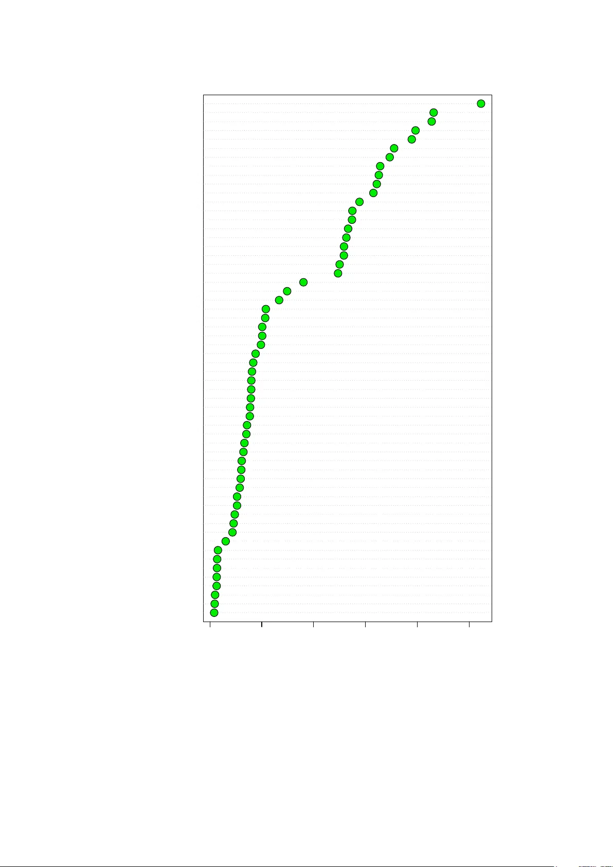
Human diffusion and cit y influence Maxime Lenormand, 1 Bruno Gon¸ calv es, 2 An t` onia T ugores, 1 and Jos ´ e J. Ramasco 1 1 Instituto de F ´ ısic a Inter disciplinar y Sistemas Complejos IFISC (CSIC-UIB), 07122 Palma de Mal lor c a, Sp ain 2 Aix Marseil le Universit´ e, Universit´ e de T oulon, CNRS, CPT, UMR 7332, 13288 Marseil le, F r anc e Cities are c haracterized by concentrating p opulation, economic activity and services. Ho wev er, not all cities are equal and a natural hierarch y at lo cal, regional or global scales sp ontaneously emerges. In this work, w e introduce a method to quantify city influence using geolocated t weets to c haracterize human mobilit y . Rome and Paris appear consistently as the cities attracting most div erse v isitors. The ratio b etw een lo cals and non-lo cal visitors turns out to b e fundamental for a cit y to truly b e global. F o cusing only on urban residents’ mobility flows, a cit y to city net work can b e constructed. This net work allo ws us to analyze centralit y measures at differen t scales. New Y ork and London pla y a predominan t role at the global scale, while urban rankings suffer substantial c hanges if the fo cus is set at a regional level. Ev er since Christaller prop osed the central place theory in the 30’s [ 1 ], researchers hav e work ed to un- derstand the relations and comp etition b etw een cities leading to the emergence of a hierarch y . Christaller en visioned an exclusive area surrounding each cit y at a regional scale to which it provided services such as mark ets, hospitals, schools, univ ersities, etc. The ser- vices displa y different level of sp ecialization, induc- ing thus a hierarch y among urban areas according to the type of services offered. In addition, this idea naturally brings an equidistant distribution of urban cen ters of similar category as long as no geographical constrain ts preven ts it. Still, in the present global- ized world relations b etw een cities go muc h b eyond mere geographical distance. In order to take into ac- coun t this fact, it was necessary to introduce the con- cept of world city [ 2 ]. These are cities that concen- trate economic w arehouses like the headquarters of large m ultinational companies or global financial dis- tricts, of kno wledge and innov ation as the cutting edge tec hnological firms or univ ersities, or p olitical decision cen ters, and that play an eminen t role of dominance o ver smaller, more local, counterparts. The concept of global city is, nevertheless, v ague and in need of fur- ther mathematical formalization. This is attained b y means of so-called world city net works, in which eac h pair of cities is linked whether they share a common resource or in terchange go o ds or p eople [ 3 – 7 ]. F or in- stance, a link can b e established if tw o cities share headquarters of the same compan y [ 7 – 9 ], if b oth are part of go o d pro duction chains [ 10 ], interc hange fi- nance services [ 11 ], internet data [ 12 ] or if direct flights or boats connect them [ 4 , 13 – 15 ]. Ce n trality measures are then applied to the netw ork and a ranking of the cities naturally emerges. Due in great part to their geographical lo cations and traditional roles as trans- A tlantic bridges, New Y ork and London are typically the top rankers in many of these studies [ 5 , 9 , 14 ]. There are, how ever, inconsistencies in terms of the meaning and stabilit y of the results obtained from dif- feren t netw orks or with differen t cen trality measures [ 14 , 16 ] and a more organic and stable definition is needed. Here we use information and communication tech- nologies (ICT) to approach the problem from a differ- en t persp ectiv e. How long w ould information originat- ing from a given city require to reac h any other city if w ere to pass from p erson to p erson only through face to face con versations? Or, in other words, what is the lik eliho o d that that information reac hes a certain dis- tance aw a y after a given time p erio d. In this though t exp erimen t, the most c entr al place in the world w ould simply b e the one where the message can reach ev- erywhere else in the shortest amount of time. This view allows us to easily define a temp oral netw ork of influence. W e p erform this analysis b y empirically observing ho w people tra v el w orldwide and using that as a pro xy for ho w quickly our message would be able to spread. The recent p opularization and affordability of geolo- cated ICT services and devices suc h as mobile phones, credit or transp ort cards gets registered generating a large quan tity of real time data on how p eople mo ve [ 17 – 25 ]. This information has been used to study questions such as interactions in so cial netw orks [ 26 – 29 ], information propagation [ 30 ], city structure and land use [ 23 , 31 – 40 ], or ev en road and long range train traffic [ 41 ]. It is bringing a new era in the so-called Sci- ence of Cities by providing a ground for a systematic comparison of the structure of urban areas of differen t sizes or in differen t countries [ 37 , 38 , 40 , 42 – 47 ]. Data coming from credit cards and mobile phones are usu- ally constrained to a limited geographical area such as a cit y or a country , while those coming from on- line so cial media as Twitter, Flic kr or F oursquare can refer to the whole glob e. This is the reason why we fo cus here on geolo cated tw eets, which hav e already pro ven to b e an useful to ol to analyze mobility b e- t ween countries [ 48 ] and provide the ideal framew ork for our analysis. In particular, w e select 58 out of the most p opulated cities of the w orld and analyze their influence in terms of the av erage radius tra veled and the area co vered b y Twitter users visiting each of them as a function of time. Differences in the mobility for lo cal residents and external visitors are taken into account, in such a w ay that cities can b e ranked according to the exten- sion cov ered by the diffusion of visitors and residents, 2 Figure 1 : Positions of the geolo cated t weets. Each t weet is represented as a p oint on the map lo cation from whic h it was p osted. tak en b oth together and separately , and by the at- tractiv eness they exhibit tow ards visitors. Finally , we also consider the interaction b etw een cities, forming a netw ork that provide a framework to study urban comm unities and the role cities play within their own comm unity (regional) versus a global p ersp ectiv e. MA TERIALS AND METHODS Twitter Dataset Our database con tains 21 , 017 , 892 tw eets geolo- cated worldwide written by 571 , 893 users in the tem- p oral p erio d ranging from Octob er 2010 to June 2013 (1000 days). There are on av erage 36 t weets p er user. Non-h uman b eha viors or collectiv e accoun ts ha ve been excluded from the data by filtering out users trav el- ing faster than a plane (750 km/h). F or this, w e ha ve computed the distance and the time sp ent b etw een t wo successive geolo cated tw eets p osted by the same user. The geographical distribution of tw eets is plot- ted in Figure 1 . The distribution matches p opulation densit y in many countries, although it is imp ortant to note that some areas are under-represented as, for example, most of Africa and China. W e take as reference 58 cities around the w orld (see T able S1 in App endix for a detailed accoun t) that are b oth highly p opulated (most are among the 100 most p opulated cities in the world) and hav e a sufficien tly large num b er of geolo cated Twitter users. T o a void distortions imp osed by different spatial scales and ur- ban area definitions that can b e problematic [ 49 , 50 ], w e op erationally defined each city to b e a circle of radius 50 km around the resp ective City Hall. In order to assess the influence of a cit y , we need to characterize how users trav el after visiting it. T o do so, we consider the tw eets p osted by user υ ∆ t da ys after visiting city c . In Figure 2 , the lo cations of geolo cated t w eets are plotted according to the num ber of da ys since the first visit in Paris and New Y ork as an example. Not surprisingly , a large part of the t weets are concentrated around these cities but one can observe ho w use rs even tually diffuse worldwide. Starting from Paris Starting from New Y ork a b Figure 2 : Geolo cated tw eets of users who ha ve b een at least once in Paris (a) and New Y ork (b). The color changes according to the num ber of days ∆ t since the first passage in the city . In red, one da y; In yel- lo w, b etw een 1 and 10 days; In green, b etw een 10 and 100 da ys; And in blue, more than 100 days. Definition of the user’s place of residence T o identify the Twitter users’ place of residence, we start by discretizing the space. T o do so, we divide the world using a grid comp osed of 100 × 100 square kilometers cell in a cylindrical equal-area pro jection. In total there are appro ximately 5 , 000 inhabited cells in our dataset. The place of residence of a user is a priori given by the cell from whic h he or she has p osted most of his/her tw eets. Ho w ever, to av oid selecting users who did not show enough regularity , w e consider only those users who posted at least one third of their t weets form the place of residence (representing more than 95% of the ov erall users). F or eac h city , the n umber of v alid users as well as the n umber of tw eets p osted from their first passage in the cit y are pro vided in T able S1 in App endix. W e can no w determine for eac h city if a user is res- iden t (local user) or a visitor (non-local user). T o do so, we compute the a verage p osition of the tw eets p osted from his/her cell of residence. If this p osition falls within the cit y b oundaries (circle of radius 50 km around the City Hall) the use r is considered as a lo cal and as a non-lo cal user otherwise. 3 ∆ t ( d a ys) R ( k m ) 10 0 10 1 10 2 10 3 10 1 10 2 10 3 10 4 Ho ng K o ng P a r is Lo nd o n D e t ro it B a nd ung ~ Δ t 1/2 ~ Δ t Figure 3 : Ev olution of the av erage radius. Eac h curv e represents the evolution of the a verage radius R av- eraged ov er 100 indep enden t extractions of a set of u = 300 users as a function of the n umber of days ∆ t since the first passage in the city . In order to sho w the general trend, eac h gray curve corresp onds to a city . The evolution of the radius for several cities is highlighted, such as the top and b ottom rankers or represen tatives of the tw o main de- tected b ehaviors. Curv es with a linear and square ro ot gro wth are also shown as a guide to the eye. The dashed lines represent the standard deviation. Metrics to assess cit y influence W e select a fixed num ber of users u in each city at random and track their displacements in a given p e- rio d of time ∆ t since their first tw eet from it. Since the results might dep end on the sp ecific set of users c hosen, we a verage ov er 100 indep endent user extrac- tions. As sho wn in Figure S2 in Appendix, the longer ∆ t is, the low er is the p opulation of users who remain activ e, so we must establish a tradeoff b et ween num- b er of users and activit y time. Unless otherwise stated w e set u = 300 and ∆ t = 350 days in the discussion that follows. Aver age radius There are different aspects to tak e in to accoun t when trying to define ho w to prop erly measure the influence of a city due to Human Mobility . W e start our discussion by considering the av erage radius trav- eled b y Twitter users since their first t w eet from a cit y c . W e track ed for eac h user the p ositions from which he or she t weeted after visiting c , and compute the av- erage distance from these lo cations to the center of c . The av erage radius, R , is then defined as the av erage o ver all the u users of their individual radii. The a verage radius is informativ e but can b e biased b y the geograph y . Cities that are in relativ ely isolated p ositions such as islands may ha ve a high av erage ra- dius just b ecause a long trip is the only option to tra vel to them. T o a void this effect, we define the normal- ized av erage radius ˜ R of a city c as the ratio b etw een R ( c ) and the av erage distance of all the Twitter users’ places of residence to c (Figure S4 in App endix). Cover age One p ossible wa y to ov ercome the limitation of the a verage ratio defined ab o ve is to discard geographic coherence all together and simply measure the geo- graphical area cov ered by those users, regardless of the distance at whic h it might b e lo cated from the originating city . In order to estimate the area cov er b y the users, the world surface has b een divided in cells of 100 × 100 square kilometers as we hav e done to identify the users’ place of residence. By trac king the mov emen ts of the set of users passing through each cit y , we count the num ber of cells from whic h at least a tw eet has b een p osted and define cov erage as this n umber. This metric has the clear adv an tage of not b eing sensitive to isolated lo cations but it still do es not consider how sp ecific cells, sp ecially the ones cor- resp onding to other important cities, are visited m uc h more often than others. RESUL TS Comparing the influence of cities W e start by taking the p ersp ective from the city to the world and compare how effective the cities are as starting p oints for the Twitter users’ diffusion. The ev olution of the av erage radius as a function of the time is plotted in Figure 3 for the 58 cities. The curv es of the log-log plot show an initial fast increase follow ed b y a muc h slo wer growth after approximately 15 − 20 da ys. The presence of these t w o regimes is mainly due to the presence of non-local users as it can b e observed in Figure S5 in App endix. In the initial phase, the ra- dius grows for all the cities at a rhythm faster than the square ro ot of time, which is the classical predic- tion for 2 D Wiener diffusion [ 51 ]. This is not fully surprising since the users’ mobility is b etter describ ed b y Levy flights than b y a Wiener process. Still the dif- ferences b etw een cities are remark able. There are t wo main b ehaviors: the radius for cities such as Detroit gro ws slowly , while others like P aris show an increase that is close to linear. After this initial transient, the a verage radius enters in a regime of slow gro wth for all the cities that is even slo wer than √ ∆ t . This im- plies that the long displacemen ts b y the users are con- cen trated in the first month, p erio d during which the non-lo cal users come back home, after which the ex- ploration b ecomes more lo calized. Ev en though the curv es of differen t cities ma y cross in the first regime, 4 30 32 34 36 38 40 42 New Y ork Shanghai San Francisco T aipei Lisbon Beijing Paris Rome Sydney Hong K ong R (x 10 3 km) a 0.35 0.40 0.45 0.50 Miami V ancouver Beijing Barcelona New Y ork Hong K ong San Francisco Lisbon Paris Rome R ~ b 520 540 560 580 600 620 Hong K ong Phoenix Brussels Barcelona Dallas Shanghai Beijing Lisbon Paris Rome Cov erage c Figure 4 : Rankings of the cities according to the av erage radius and the cov erage. (a) T op 10 cities ranked b y the av erage radius R . (b) T op 10 cities ranked by the normalized av erage radius ˜ R . (c) T op 10 cities ranked by the co verage (num ber of visited cells). All the metrics are av eraged ov er 100 indep enden t extractions of a set of u = 300 users. they reach a relativ ely stable configuration in the sec- ond one. W e can see that the top ranker in terms of capacit y of diffusion is Hong Kong for the whole time windo w considered and the b ottom one is Bandung (W est Jav a, Indonesia). The top 10 cities according to the av erage radius are plotted in Figure 4 a. It is w orth noting New Y ork only app ears in the last position, in con trast to previously published rankings based on different data [ 5 , 9 , 14 ]. Many cities on the top are in the Pa- cific Basin (Hong-Kong, Sydney , Beijing, T aip ei, San F rancisco and Shanghai), which is clear evidence for the impact of geography on R . W e take geographical effects into account b y calculating the normalized ra- dius ˜ R as shown in Figure 4 b. With this correction, the top cities are Rome, Paris and Lisb on. These cities are located in densely p opulated Europ e but still man- age to send trav elers further a wa y than any other, a pro of for their aptitude as sources for the informa- tion spreading thought exp eriment describ ed in the in tro duction. Actually , all cities in the T op 10 set are also able to attract visitors at a worldwide scale, some are relativ ely far from other global cities and/or they may b e the gate to extensive hin terlands (China). The same ranking for the cov erage is shown in Figure 4 c. Even though these tw o metrics are strongly corre- lated (see Figure S6 in Appendix) there are still some significan t differences indicating that they are able to capture different information. The top cities, ho w ev er, are again Rome, P aris and Lisb on probably due to a com bination of the factors explained ab o ve. It should also b e noted that even though the users extraction is sto c hastic and the rankings can v ariate slightly from a realization to another (see Figure S7 in App endix), the ranking is stable when p erformed on the av erage o ver several realizations it b ecomes stable (Figure S8 in App endix). Lo cal versus non-lo cal Twitter users W e ha ve y et to tak e into account that individual re- siding in a city might behav e differently from visitors. 50 100 150 200 250 300 350 0.1 0.2 0.3 0.4 0.5 0.6 Cover age R ~ Local Non−Local a 100 200 300 400 500 600 0.2 0.3 0.4 0.5 0.6 0.7 0.8 Proportion of Non−Local Users Cover age b 125 135 145 155 New Y ork Chicago San Francisco Shanghai Dallas Berlin Paris Saint Peter sburg Beijing Moscow Cover age c 325 335 345 Houston Barcelona Brussels Detroit Lima Istanbul Rome Moscow Paris Lisbon Cover age d Figure 5 : Relation b et ween local and non-lo cal users. (a) Scatter-plot of ˜ R as a function of the cov er- age for locals (blue triangles) and non-lo cals (red squares). (b) Cov erage as a function of the prop ortion of non-lo cal Twitter users. (c) T op 10 ranking cities based only on lo- cal users according to the co verage. (d) The same ranking but based only on the mo vemen ts of non-lo cal users. In all the cases, the num ber of lo cal and non-lo cal users ex- tracted is u = 100 for every city and all the metrics are a veraged ov er 100 indep endent extractions. W e consider a user to be a resident of a city if most of his/her tw eets are p osted from it. Otherwise, he/she is seen as an external visitor. Residents of the 58 cities w e consider hav e a significantly lo wer co v erage (ab out 96) than visitors (ab out 260). This means that the lo- cals mo ve to ward more concentrated lo cations, suc h as places of work or the residences of family and friends, while visitors hav e a comparativ ely higher diversit y of origins and destinations. The difference betw een locals and non-locals is ev en more dramatic when the normalized radius, ˜ R , for eac h cit y is plotted as a function of the co verage for b oth t yp es of users in Figure 5 a. Two clusters clearly emerge, sho wing that the lo cals tend to mo ve less than 5 the visitors. Such difference b etw een users is lik ely to b e behind the change of b eha vior in the temporal evo- lution of the av erage radius detected in Figure 3 , and in tro duces the ratio of visitors ov er lo cal users as a rel- ev an t parameter to describ e the mobility from a city . Indeed, visitors con tribute the most for the radius and the area cov ered (see Figure 5 b for the co verage) while residen ts contribute most to the lo cal relev ance of a cit y (Figure 5 c for the cov erage and Figure S10a in Ap- p endix for ˜ R ). The top rankers in this classification are Hong Kong and San F rancisco in ˜ R and Moscow and Beijing in the cov erage. All of them are cities that may act as gates for quite extense hin terlands. The rankings based on non-lo cals (Figures 5 d for the co verage and Figure S10b in App endix for ˜ R ) get us bac k the more common top rank ers suc h as P aris, New Y ork and Lisb on. Cit y attractiveness Th us far, w e hav e considered a city as origin and an- alyzed how people visiting it diffuse across the planet. W e no w consider the attractiv eness of a cit y b y taking the opp osite p oint of view and analyzing the origins of each user seen within the confines of a city . W e mo dify the tw o metrics defined ab ov e to consider the normalized av erage distance of the users’ residences (represen ted by the centroid of the cell of residence) to the center of the considered city c and the num b er of differen t cells where these users come from. In this case, the to metrics are av eraged ov er 100 indep en- den t extractions of u = 1000 Twitter users. The re- sulting rankings depict the attractiv eness of each city from the p ersp ective of external visitors: How far are p eople willing to trav el to visit this city? The T op 10 cities are shown in Figure 6 for the cov erage (see Figure S11 in App endix for the normalized a verage radius). Rome, Paris and Lisb on are also quite con- sisten tly the top rankers in terms of attractiveness to external visitors. A netw ork of cities Finally , w e complete our analysis by considering tra vel b etw een the 58 selected cities. W e build a net work connecting the 58 cities under consideration where the directed edge from city i to city j has a w eight given by the fraction of lo cal Twitter users in the city i which were observed at least once in city j . F or simplicity , in what follows, we consider only lo cal users who left their city at least once. This net work captures the strength of connections betw een cities al- lo wing us to analyze the communities that naturally arise due to human mobility . Using the OSLOM clus- tering detection algorithm [ 52 , 53 ] we find 6 commu- nities as sho wn in Figure 7 . These comm unities follo w appro ximately the natural b oundaries b etw een conti- nen ts: tw o communities in North and Center America, 210 230 250 270 Shanghai New Y ork Dallas Miami Beijing Berlin Lisbon Barcelona P aris Rome Number of Cells of Residence Figure 6 : City attractiveness. T op 10 cities ranked b y the num ber of distinct cells of residence for u = 1000 Twitter users drawn at random. The metric is av eraged o ver 100 independent extractions. one communit y in South America, another in Europ e, t wo communities in Asia (Japan and rest of Asia plus Sydney), indicating that they correspond to economic, cultural and geographical pro ximities. Similar results w ere obtained using the Infomap [ 54 ] cluster detection algorithm, confirming the robustness of the communi- ties detected. North America Global Ranking Regional Ranking 1. New Y ork (1) 1. New Y ork 2. Miami (6) 2. Los Angeles 3. San F rancisco (8) 3. Chicago 4. Los Angeles (9) 4. T oronto 5. Chicago (18) 5. Detroit 6. T oronto (19) 6. Miami 7. San Diego (23) 7. Dallas 8. Detroit (25) 8. San F rancisco 9. Montreal (26) 9. W ashington 10. Atlan ta (27) 10. Atlan ta Europ e Global Ranking Regional Ranking 1. London (2) 1. London 2. Paris (3) 2. Paris 3. Madrid (10) 3. Moscow 4. Barcelona (11) 4. Barcelona 5. Moscow (16) 5. Berlin 6. Berlin (20) 6. Rome 7. Rome (21) 7. Madrid 8. Amsterdam (24) 8. Lisb on 9. Lisb on (38) 9. Amsterdam 10. Milan (40) 10. Saint Petersburg T ABLE I: Comparison of the regional and the global b et weenness rankings. In parenthesis the total global ranking p osition of eac h cit y . With these empirical communities in hand we can no w place each city into a lo cal as well as a global 6 0 2 46 8 10 Los Angeles San Francisco M iami Sin gapore T ok yo Pa ris London Ne w York Weight ed Betwennness (x 10 2 ) Weight ed degree Figure 7 : Mobilit y netw ork. Lo cal Twitter users mobility net w ork b etw een the 58 cities. Only the flo ws representing the top 95% of the total flo w hav e b een plotted. The flows are drawn from the least to the greatest. The inset shows the top 8 cities ranked by weigh ted b etw eenness and weigh ted degree. con text. In a netw ork con text, the imp ortance of eac h no de can b e measured in different w ays. Tw o classi- cal measures are the strength of a no de [ 55 ] and the w eighted b etw eenness [ 56 , 57 ]. Giv en the wa y we de- fined our netw ork ab ov e, these corresp ond, roughly , to the fraction of lo cal users that tra vel out of a city and how imp ortant that city is in connecting trav- elers coming from other cities to their final destina- tions. In the inset of the Figure 7 , w e analyze the ranking resulting from these t wo metrics and iden- tify New Y ork and London as the most central no des in terms of degree and b etw eenness and, particularly , New Y ork for the weigh ted degree at a global scale. Ho wev er, when we restrict our analysis to just the regional scene of each communit y , the relative imp or- tance of each city quickly changes. The rankings for the regional w eighted degree are similar to the global ones since this metric dep ends only on the p opulation of each city and not on who it is connected to. The most central cities o ccupy the same p ositions except for San Diego, which slipped do wn three places down. On the other hand, the weigh ted betw eenness is prop- ert y that dep ends strongly on the netw ork top ology , a prop erty that can b e seen by the dramatic shifts w e observe when considering only the lo cal comm u- nit y of each cit y with most cities moving several p o- sitions up or do wn (see details in T able I I and T a- ble S2 in App endix). F or example, San Diego wen t do wn nine places meaning that this city has a global influence due to the fact that San Diego is a com- m unication hub b etw een United States and Central America. Dallas wen t up six places, indicating that its influence is higher at the regional scale rather than in the international arena. In the same wa y , Madrid w ent down four places whereas Barcelona stay ed at the same place, this means that Madrid is more in- fluen tial than Barcelona at a global scale as an inter- national bridge connecting Europ e and Central and South America but not at a regional (Europ ean) scale. DISCUSSION The study of comp etition and in teractions b etw een cities has a long history in fields such as Geography , Spatial Economics and Urbanism. This research has traditionally tak en as basis information on finance ex- c hanges, sharing of firm headquarters, n umber of pas- sengers transp orted by air or tons of cargo dispatc hed from one cit y to another. One can define a netw ork relying on these data and identify the so-called W orld Cities, those with a higher level of centralit y as the global economic or logistic centers. Here, we hav e tak en a radically different approach to measure quan- titativ ely the influence of a city in the world. No w a- da ys, geolo cated devices generate a large quantit y of real time and geolo cated data p ermitting the char- acterization of p eople mobility . W e ha ve used Twit- ter data to track users and classify cities according to the mobility patterns of their visitors. T op cities as mobility sources or attraction p oints are iden tified as central places at a global scale for cultural and in- formation interc hanges. This definition of cit y influ- ence mak es p ossible its direct measurement instead of using indirect information such as firm headquar- ters or direct flights. Still, the quality of the results dep ends on the capacity of geolo cated tw eets to de- scrib e local and global mobilit y . Indeed, observing the W orld through Twitter data can lead to p ossible dis- tortions, economic and so cio demographic biases, the 7 Twitter p enetration rate may also v ary from country to country leading to an under-representation of the p opulation, for example, from Africa and from China. The cities selected for this w ork are those that, on one hand, concen trate large populations and, on the other, enough num ber of tw eets to b e part of the analysis. There are biases acting against our work, as the lack of cov erage in some areas of the w orld, and others in fav or, such as the fact that younger and w ealth- ier individuals are more likely to b oth tra vel and use Twitter. The estimated mobilit y patterns are nat- urally partial since only refer to the selected cities. Still, as long as the users provide a significant sam- ple of the external urban mobility , the flow netw ork is enough for the p erformed analysis. F urthermore, sev- eral recent works ha ve prov en the capacity of geolo- cated tw eets to describ e human mobility comparing differen t data sources as information collected from cell phone records, Twitter, traffic measure tec hniques and surveys [ 23 , 24 , 41 ]. More sp ecifically and assuming data reliabilit y , we consider the users’ displacements after visiting each cit y . The urban areas are ranked according to the area cov ered and the radius trav eled b y these users as a function of time. These metrics are inspired b y the framework dev elop ed for random walks and Levy fligh ts, which allows us to characterize the evolution of the system with well-defined mathematical to ols and with a clear reference baseline in mind. Previ- ous literature rankings usually find a hierarch y cap- tained by New Y ork and London as the most central w orld cities. The ranks dramatically c hange when one has into account users’ mobility . A triplet formed by Rome, Paris and Lisb on consistently app ear on the top of the ranking b y extension of visitor’s mobility but also by their attractiveness to trav elers of very div erse origin. A combination of economic activity app ealing to tourism and diversit y of links to other lands, in some cases pro duct of recent history , can ex- plain the presence of these cities on the top. These three cities are follow ed by others such as San F ran- cisco that without b eing one of the most p opulated cities in the US extends it influence ov er the large P a- cific basin or Hong Kong, Beijing and Shanghai that replicates it on the other side of the Pacific region. These cities are in some cases gates to broad hinter- lands. This is relev an t since our metrics hav e into accoun t the diversit y in the visitors’ origins. These results rely on the full users p opulation, dis- criminating only by the place of residence b etw een lo- cals and non lo cals to eac h cit y . The influence of cities measured in this wa y includes their impact in rural as w ell as in other urban areas. Ho w ever, the analysis can b e restricted to users residing in an urban area and to their displacemen ts tow ard other cities. In this w ay , we obtain a weigh ted directed net work b etw een cities, whose links weigh ts represen t the (normalized) fluxes of users trav eling from one cit y to another. This net work provides the basis for a more traditional cen- tralit y analysis, in which we recov er London and New Y ork as the most central cities at a global scale. The matc h b etw een our results and those from previous analysis brings further confidence on the quality of the flo w measured from online data. The netw ork framew ork p ermits to run clustering techniques and divide the world city netw ork in comm unities or ar- eas of influence. When the centralit y is studied only within each comm unity , we obtain a regional p ersp ec- tiv e that induces a new ranking of cities. The com- parison b etw een the global and the regional ranking pro vides imp ortant insights in the change of roles of cities in the hierarchies when passing from global to regional. Summarizing, we hav e introduced a new metho d to measure the influence of cities based on the Twitter user displacements as proxies for the mobility flows. The metho d, despite some p ossible biases due to the p opulation using online so cial media, allows for a di- rect measurement of a cit y influence in the w orld. W e prop osed three types of rankings capturing differ- en t p ersp ectives: rankings based on “city-to-w orld” and “world-to-cit y” in teractions and rankings based on “city-to-cit y” interaction. It is interesting to note that the most influen tial cities are very different ac- cording to the p ersp ective and the scale (regional and global). This introduces the possibility of studying re- lations among cities and b etw een cities and rural areas with unprecedented detail and scale. A CKNOWLEDGEMENTS P artial financial supp ort has b een receiv ed from the Spanish Ministry of Econom y (MINECO) and FEDER (EU) under pro jects MODASS (FIS2011- 24785) and INTENSE@COSYP (FIS2012-30634), and from the EU Commission through pro jects EUNOIA, LASA GNE and INSIGHT. The work of ML has b een funded under the PD/004/2013 pro ject, from the Con- selleria de Educacin, Cultura y Universidades of the Go vernmen t of the Balearic Islands and from the Eu- rop ean So cial F und through the Balearic Islands ESF op erational program for 2013-2017. JJR from the Ram´ on y Ca jal program of MINECO. BG was par- tially supp orted by the F rench ANR pro ject HarMS- flu (ANR-12-MONU-0018). [1] Christaller W. 1966 Die Zentralen Orte in S ¨ uddeutsc hland: eine ¨ Ok onomisch-Geographisc he Un tersuch ung ¨ Ub er die Gesetz Massigkeit der V erbreitung und Ent wic klung der Siedlungen mit St¨ adtisc hen F unktionen, Fischer V erlag, Jena (1933). (English translation: Christaller W, Baskin CW. 8 Cen tral places in Southern Germany , Prentice Hall, Englew o o d Cliffs NJ.) [2] F riedmann J, W olff G. 1982 W orld cit y formation: an agenda for research and action. International Jour- nal of Urb an and R e gional R ese ar ch 6 , 309–344. (doi:10.1111/j.1468-2427.1982.tb00384.x) [3] Berry B. 1964 Cities as systems within a systems of cities. Papers of R e gional Science Asso ciation 13 , 147–163. (doi:10.1111/j.1435-5597.1964.tb01283.x) [4] Knox PL, T aylor PJ. 1995 W orld cities in a world- system. Cambridge Universit y Press. [5] Rimmer P . 1998 T ransp ort and T elecommunications among world cities. In Lo FC, Y eung YM (eds.). Glob- alization and the world of lar ge cities , T okyo: United Nations Universit y Press, 433–470. [6] Pumain D. 2000 Settlemen t systems in the evolution. Ge o gr afiska A nnaler 82B , 73–97. (doi:10.1111/j.0435- 3684.2000.00075.x) [7] T aylor JP . 2001 Specification of the W orld Cit y Net work. Ge o gr aphic al Analysis 33 , 181–194. (doi:10.1111/j.1538-4632.2001.tb00443.x) [8] Derudder B, T aylor PJ, Witlox F, Catalano G. 2003 Hierarc hical tendencies and regional patterns in the world city netw ork: A global urban anal- ysis of 234 cities. R e gional Studies 37 , 875–886. (doi:10.1080/0034340032000143887) [9] Derudder B, Witlox F. 2004 Assessing central places in a global age: on the netw orked lo calization strate- gies of adv ances pro ducer services. J. R etailing and Consumer Servic es 11 171–180. (doi:10.1016/S0969- 6989(03)00023-7) [10] Brown E, Derudder B, Parnreiter C, Pelupessy W, T aylor PJ, Witlox F. 2010 W orld City Netw orks and Global Commo dity Chains: to wards a w orld- systems’ in tegration. Glob al Networks 10 , 1470–2266. (doi:10.1111/j.1471-0374.2010.00272.x) [11] Bassens D, Derudder B, Witlox F. 2010 Search- ing for the Mecca of finance: Islamic financial ser- vices and the world city netw ork. Ar e a 42 , 35–46. (doi:10.1111/j.1475-4762.2009.00894.x) [12] Neal Z. 2011 Differentiating centralit y and p ow er in the world cit y netw ork. Urb an Studies 48 , 2733–2748. (doi:10.1177/0042098010388954) [13] Zo ok MA, Brunn SD. 2005 Hierarchies, Regions and Legacies: Europ ean cities and global commercial pas- senger air trav el. J. Contemp or ary Eur op e an Studies 13 , 203–220. (doi:10.1080/14782800500212459) [14] Derudder B, Witlox F. 2005 On the use of inad- equate airline data in mappings of a global urban system. J. Air T r ansp ort Management 11 , 231–237. (doi:10.1016/j.jairtraman.2005.01.001) [15] Derudder B, Witlox F. 2008 Mapping world city net works through airline flows: context, relev ance, an problems. J. T ransp ort Geo gr aphy 16 , 305–312. (doi:10.1016/j.jtrangeo.2007.12.005) [16] Allen J. 2010 P ow erful city net works: More than connections, less than domination and con trol. Urb an Studies 47 , 2895–2911. (doi: 10.1177/0042098010377364) [17] Bro c kmann D, Hufnagel L, Geisel T. 2006 The scal- ing laws of human trav el. Natur e 439 , 462–465. (doi:10.1038/nature04292) [18] Gonzalez MC, Hidalgo CA, Barabasi A-L. 2008 Un- derstanding individual human mobility patterns. Na- tur e 453 , 779–782. (doi:10.1038/nature06958) [19] Balcan D, Colizza V, Gon¸ calv es B, Hu H, Ram- asco JJ, V espignani V. 2009 Multiscale mobility net- w orks and the spatial spreading of infectious dis- eases. Pr o c. Natl. A c ad. Sci. USA 106 , 21484–21489. (doi:10.1073/pnas.0906910106) [20] Noulas A, Scellato S, Lambiotte R, Pon til M, Mas- colo C. 2012 A tale of many cities: Universal pat- terns in human urban mobility . PloS one 7 , e37027. (doi:10.1371/journal.p one.0037027) [21] Bagrow JP , Lin Y-R. 2012 Mesoscopic structure and so cial asp ects of human mobility . PLoS ONE 7 , e37676. (doi:10.1371/journal.p one.0037676) [22] Grab o wicz P A, Ramasco JJ, Goncalves B, Eguiluz VM. 2014 En tangling mobility and interac- tions in social media. PL oS ONE 9 , e92196. (doi:10.1371/journal.p one.0092196) [23] Lenormand M, Picornell M, Garcia Cant´ u O, T u- gores A, Louail T, Herranz R, Barthelemy M, F r ´ ıas- Mart ´ ınez E, Ramasco JJ. 2014 Cross-chec king dif- feren t source of mobility information. PL oS ONE 9 , e105184. (doi:10.1371/journal.p one.0105184) [24] Tizzoni M, Ba jardi P , Decuyper A, Kon Kam King G, Schneider CM, Blondel V, Smoreda Z, Gonzlez MC, Colizza V. 2014 On the use of h uman mobilit y proxy for the mo deling of epi- demics. PL oS Computational Biolo gy 10 , e1003716. (doi:10.1371/journal.p cbi.1003716) [25] Jurdak R, Zhao K, Liu J, Ab ouJaoude M, Cameron M, Newth D. 2014 Understanding h u- man mobilit y from Twitter. Av ailable online at h ttp://arxiv.org/abs/1412.2154 . [26] Jav a A, Song X, Finin T, Tseng B. 2007 Wh y w e t witter: understanding microblogging usage and comm unities. In Pr o c e e dings of the 9th A CM WebKDD and 1st SNA-KDD 2007 workshop on Web mining and social network analysis , 56–65. (doi:10.1145/1348549.1348556) [27] Krishnamurth y B, Gill P , Arlitt M. 2008 A few chirps ab out twitter. In WOSP ’08: A CM Pr o c e e dings of the first workshop on Online so cial networks , 19–24. (doi:10.1145/1397735.1397741) [28] Hub erman BA, Romero DM, W u F. 2008 So cial netw orks that matter: Twitter un- der the microscope. First Monday 14 . ( h ttp://firstmonday .org/article/view/2317/2063 ) [29] Grab o wicz P A, Ramasco JJ, Moro E, Pujol JM, Eguiluz VM. 2012 So cial features of on- line netw orks: The strength of intermediary ties in online so cial media. PL oS ONE 7 , e29358. (doi:10.1371/journal.p one.0029358) [30] F errara E, V arol O, Menczer F, Flammini A. 2013 T rav eling trends: so cial butterflies or frequent fliers? In Pr o ce e dings of the first ACM Confer enc e on On- line So cial Networks COSN ’13 , 213–222, New Y ork. (doi:10.1145/2512938.2512956) [31] Reades J, Calabrese F, Sevtsuk A, Ratti C. 2007 Cellular census: Explorations in urban data collection. Pervasive Computing 6 , 30–38. (doi:10.1109/MPR V.2007.53) [32] Reades J, Calabrese F, Ratti C. 2009 Eigen- places: analysing cities using the space-time struc- ture of the mobile phone netw ork. Envir onment and Planning B: Planning and Design 36 , 824–836. (doi:10.1068/b34133t) [33] Cheng Z, Cav erlee J, Lee, K. 2010 Y ou Are Where Y ou Tweet: A Conten t-based Approach to Geo-lo cating Twitter Users. Pr o c e e dings of the 9 19th A CM International Confer enc e on Informa- tion and Know le dge Management 17 , 759-768. (doi:10.1080/10095020.2014.941316) [34] Soto V, F r ´ ıas-Mart ´ ınez E. 2011 Automated land use identification using cell-phone records, Pro cs. of the ACM c onfer enc e HotPlanet’11 17–22, New Y ork. (doi:10.1145/2000172.2000179) [35] F r ´ ıas-Mart ´ ınez V, Soto V, Hohw ald H, F r ´ ıas-Mart ´ ınez E. 2012 Characterizing urban landscap es using ge- olo cated tw eets. In SOCIALCOM-P ASSA T ’12 Pr o- c e e dings of the 2012 ASE/IEEE International Con- fer enc e on So cial Computing and 2012 ASE/IEEE International Confer enc e on Privacy, Se curity, Risk and T rust , 239–248. (doi:10.1109/So cialCom- P ASSA T.2012.19) [36] Noulas A, Mascol C, F rias-Martinez E. 2013 Exploit- ing F oursquare and Cellular Data to Infer User Ac- tivit y in Urban Environmen ts, Pr o cs. MDM ’13 , 167– 176. [37] Louail T, Lenormand M, Garcia Can t´ u O, Picor- nell M, Herranz R, F r ´ ıas-Mart ´ ınez E, Ramasco JJ, Barthelem y M. 2014 F rom mobile phone data to the spatial structure of cities. Scientific R ep orts 4 , 5276. (doi:10.1038/srep05276) [38] Grauwin S, Sob olevsky S, Moritz S, Go dor I, Ratti C. 2015 T o w ards a comparative science of cities: us- ing mobile traffic records in New Y ork, London and Hong Kong. In Helbich M, Jok ar Arsanjani J, Leitner M (Eds.) Computational Appr o aches for Urb an Envi- r onments 13 , 363–387. [39] F ran¸ ca U, Sa yama H, McSwiggen C, Danesh- v ar R, Bar-Y am Y. 2014 Visualizing the ”Heart- b eat” of a Cit y with Tweets. Av ailable online at h ttp://arxiv.org/abs/1411.0722 . [40] Louail T, Lenormand M, Picornell M, Garcia Cant´ u O, Herranz R, F r ´ ıas-Mart ´ ınez E, Ramasco JJ, Barthelem y M. 2015 Uncov ering the spatial struc- ture of mobility net works. Natur e Communications 6 , 6007. (doi:10.1038/ncomms7007) [41] Lenormand M, T ugores A, Colet P , Ramasco JJ. 2014 Tweets on the road. PL oS ONE 9 , e105407. (doi:10.1371/journal.p one.0105407) [42] Bettencourt L, Lob o J, Helbing D, Kuhnert C, W est G. 2007 Growth, innov ation, scaling, and the pace of life in cities. Pr o c. Natl. Ac ad. Sci. USA 104 , 7301– 7306. ( doi: 10.1073/pnas.0610172104) [43] Batty M. 2008 The Size, Scale, and Shap e of Cities. Scienc e 319 , 769–771. (doi:10.1126/science.1151419) [44] Bettencourt L, W est G. 2010 A unified the- ory of urban living. Natur e 467 , 912–913. (doi:10.1038/467912a) [45] Bettencourt L. 2013 The Origins of Scal- ing in Cities. Scienc e 340 , 1438–1441. (doi:10.1126/science.1235823) [46] Adnan A, Leak A, Longley P . 2014 A geo computa- tional analysis of Twitter activit y around different w orld cities. Ge o-sp atial Information Scienc e 17 , 145- 152. (doi:10.1080/10095020.2014.941316) [47] Batty M. 2013 The New Science of Cities. The MIT Press. [48] Haw elk a B, Sitko I, Beinat E, Sob olevsky S, Kaza- k op oulos P , Ratti C. 2014 Geo-located twitter as a pro xy for global mobilit y patterns. Carto gr aphy and Ge o gr aphic Information Scienc e 41 , 260–271. (doi:10.1080/15230406.2014.890072) [49] Oliveira EA, Andrade Jr JS, Makse HA. 2014 Large cities are less green. Scientific R ep orts 4 , 4235. (doi:10.1038/srep04235) [50] Arcaute E, Hatna E, F erguson P , Y oun H, Jo- hansson A, Batty M. 2015 Constructing cities, de- constructing scaling la ws. J. R. So c. Interfac e 12 . (doi:10.1098/rsif.2014.0745) [51] W eiss, GH. 1994 Asp ects and Applications of the Ran- dom W alk. North-Hol land Publishing Co. [52] Lancichinetti A, Radicc hi F, Ramasco JJ. 2010 Statistical significance of communi- ties in netw orks. Phys. R ev. E 81 , 046110. (doi:10.1103/Ph ysRevE.81.046110) [53] Lancichinetti A, Radicc hi F, Ramasco JJ, F or- tunato S. 2011 Finding Statistically Significant Comm unities in Net works. PLoS ONE 6 , e18961. (doi:10.1371/journal.p one.0018961) [54] Rosv all M, Bergstrom CT. 2008 Maps of random w alks on complex netw orks reveal communit y struc- ture. Pr o c. Natl. A c ad. Sci. USA 105 , 1118–1123. (doi:10.1073/pnas.0706851105) [55] Barrat A, Barthelemy M, Pastor-Satorras R, V espig- nani A. 2004 The architecture of complex weigh ted net works. Pr o c. Natl. A c ad. Sci. USA 101 , 3747–3752. (doi:10.1073/pnas.0400087101) [56] Newman MEJ. 2001 Scien tific collab oration net works. I I. Shortest paths, weigh ted net- w orks, and centralit y . Phys. R ev. E 64 , 016132. (doi:10.1103/Ph ysRevE.64.016132) [57] Brandes U. 2001 A faster algorithm for b e- t weenness centralit y . J. Math. So c. 25 , 163–177. (doi:10.1.1.11.2024) 10 APPENDIX As a first characterization of the data, w e ha ve computed the great circle distance ∆ r b et ween successiv e p ositions of the same Twitter user living in one of the 58 cities (Figure S1). The distribution P (∆ r ) for each cit y is well approximated by a p ow er law with an av erage exp onen t v alue of 1 . 5. These results are consistent with the exp onent obtained in other studies [ 17 , 18 , 48 ]. It is interesting to note that the distributions are v ery similar for all the cities. ● ● ● ● ● ● ● ● ● ● ● ● ● ● ● ● ● ● ● ● ● ● ● ● ● ● ● ● ● ● ● ● ● ● ● ● ● ● ● ● ● ● ● ● ● ● ● ● ● ● ● ● ● ● ● ● ● ● ● ● ● ● ● ● ● ● ● ● ● ● ● ● ● ● ● ● ● ● ● ● ● ● ● ● ● ● ● ● ● ● ● ● ● ● ● ● ● ● ● ● ● ● ● ● ● ● ● ● ● ● ● ● ● ● ● ● ● ● ● ● ● ● ● ● ● ● ● ● ● ● ● ● ● ● ● ● ● ● ● ● ● ● ● ● ● ● ● ● ● ● ● ● ● ● ● ● ● ● ● ● ● ● ● ● ● ● ● ● ● ● ● ● ● ● ● ● ● ● ● ● ● ● ● ● ● ● ● ● ● ● ● ● ● ● ● ● ● ● ● ● ● ● ● ● ● ● ● ● ● ● ● ● ● ● ● ● ● ● ● ● ● ● ● ● ● ● ● ● ● ● ● ● ● ● ● ∆ r ( km ) P ( ∆ r ) 10 0 10 1 10 2 10 3 10 4 10 −7 10 −6 10 −5 10 −4 10 −3 10 −2 10 −1 ● ● ● ● ● Philadelphia London New Y ork W ashington Bruxelles a −1.8 −1.7 −1.6 −1.5 −1.4 −1.3 −1.2 P ower la w e xponent b 0.90 0.92 0.94 0.96 0.98 1.00 R 2 c Figure S1 : Probablity density function of distance trav elled by the lo cal Twitter users. (a) Probablity densit y function P (∆ r ) of the distance trav elled by the lo cal Twitter users for 5 cities drawn at random among the 58 case studies. ∆ r is the great circle distance b etw een each successive position of the lo cal Twitter users. (b) Boxplot of the 58 pow er-law exp onent. (c) Boxplot of the R 2 . The b oxplot is comp osed of the minimum v alue, the low er hinge, the median, the upp er hinge and the maxim um v alue. 200 400 600 800 1000 0 200 400 600 800 ∆ t (da y) Number of activ e users ● (350,300) Figure S2 : Minim um n umber of activ e users as a function of ∆ t (blue line). The gra y lines represent the n umber of active users as a function of ∆ t for the 58 cities. 11 ● ● ● ● ● ● ● ● ● ● ● ● ● ● ● ● ● ● ● ● ● ● ● ● ● ● ● ● ● ● ● ● ● ● ● ● ● ● ● ● ● ● ● ● ● ● ● ● ● ● ● ● ● ● ● ● ● ● ● ● ● ● ● ● ● ● ● ● ● ● ● ● ● ● ● ● ● ● ● ● ● ● ● ● ● ● ● ● ● ● ● ● ● ● ● ● ● ● ● ● ● ● ● ● R (km) P ( R ) 10 0 10 1 10 2 10 3 10 4 10 −6 10 −5 10 −4 10 −3 10 −2 a ● ● ● ● ● Rome P aris New Y ork Lisbon London ● ● ● ● ● ● ● ● ● ● ● ● ● ● ● ● ● ● ● ● ● ● ● ● ● ● ● ● ● ● ● ● ● ● ● ● ● ● ● ● ● ● ● ● ● ● ● ● ● ● ● ● ● ● ● ● ● ● Ranking A v erage Ranking Median 0 10 20 30 40 50 60 0 10 20 30 40 50 60 b Figure S3 : Radius. (a) Probablity densit y function of the radius p er Twitter users for 5 cities. (b) Ranking by median radius as a function of the ranking by av erage radius. The rankings are based on an av erage of the t wo statistics ov er 100 indep endent extractions of a set of u = 300 users. 12 70 80 90 100 110 120 T oronto Montreal Detroit Chicago New Y ork Boston Philadelphia W ashington Atlanta Dallas Dublin Manchester Houston London Amsterdam Brussels V ancouver P aris Miami Phoenix Stockholm Berlin Los Angeles San Francisco San Diego Madrid Lisbon Milan Barcelona Saint P etersb urg Rome Mexico Guadalajara Santo Domingo Moscow Istanbul Caracas Bogota Lima Beijing Seoul T okyo Nago y a Osaka Rio de Janeiro Sao P aulo Shanghai T aipei Hong K ong Santiago Buenos Aires Bangkok Manila K uala Lumpur Singapore Jakarta Bandung Sydney A v erage Distance (x 10 3 km) Figure S4 : Ranking of the cities according the the av erage distance b etw een the center of the city and all the Twitter users’ place of residence (represented b y the cen troid of the cell of residence). 13 ∆ t (da ys) R (km) 10 0 10 1 10 2 10 3 10 1 10 2 10 3 10 4 a ∆ t (da ys) R (km) 10 0 10 1 10 2 10 3 10 1 10 2 10 3 10 4 b Hong K ong P aris London Detroit Bandung Figure S5 : Evolution of the a verage radius for the lo cal users (a) and for the non-lo cal users (b). Each curv e represents the evolution of the av erage radius R av eraged o ver 100 independent extractions of a set of u = 100 users as a function of the num ber of days ∆ t since the first passage in the city . In order to show the general trend, each gra y curve corresp onds to a city . The evolution of the radius for several cities is highlighted, such as the top and b ottom rank ers or representativ es of the tw o main detected behaviors. 0.1 0.2 0.3 0.4 0.5 100 200 300 400 500 600 R ~ Co v erage Figure S6 : Cov erage as a function of ˜ R for the 58 cities. A certain level of correlation can be observed b etw een b oth metrics. Both metrics are av eraged ov er 100 indep endent extractions of a set of u = 300 users. 14 0 5 10 15 Rank Rome P aris Lisbon San Francisco Hong K ong New Y ork Barcelona Beijing V ancouver Miami a 0 5 10 15 20 25 Rank Rome P aris Lisbon Beijing Shanghai Dallas Barcelona Brussels Phoenix Hong K ong b Figure S7 : V ariations of the rankings ov er 100 realizations. (a) Ranking for the normalized av erage radius. (b) Ranking for the cov erage. The b oxplot is comp osed of the minimum v alue, the low er hinge, the median, the upp er hinge and the maximum v alue. The rankings are av eraged ov er 100 indep endent extractions of a set of u = 300 users. 0 2 4 6 8 10 12 Rank Rome P aris Lisbon San Francisco Hong K ong New Y ork Barcelona Beijing V ancouver Miami a 0 2 4 6 8 10 12 Rank Rome P aris Lisbon Beijing Shanghai Dallas Barcelona Brussels Phoenix Hong K ong b Figure S8 : V ariations of the rankings o ver 10 realizations p erformed on the av erage ov er 10 realizations. (a) Ranking for the normalized a verage radius. (b) Ranking for the co verage. The boxplot is comp osed of the minimum v alue, the low er hinge, the median, the upp er hinge and the maxim um v alue. The rankings are av eraged ov er 100 indep enden t extractions of a set of u = 300 users. 15 En tropy index The natural wa y of taking the heterogeneity of visiting frequencies into consideration is to in tro duce an en tropy measure. If we define the probability p t i than an individual tw eet originating from the users we are considering originated in a cell i , then the entrop y S for a given time interv al ∆ t is giv en b y: S ( t ) = − P N i =1 p t i log( p t i ) log ( N ( t )) (1) where the normalizing factor N ( t ), the num ber of cells with non-zero num ber of t weets, corresp onds to the uniform case where each tw eet has the same probability of b eing pro duced within each cell. With this normalization, the en tropy is defined to v ary just b etw een 0 and 1, regardless of the nu mber of cells and t weets w e might consider in each case. The entrop y as a function of the num ber of visited cells is plotted in Figure 7 a. The entrop y enhances with the num b er of visited cells despite the normalization, which implies that the tw eets tend to distribute more uniformly for those cities with larger areas cov ered and therefore with a larger global pro jection. Besides the general trend, there are some in teresting outliers suc h as Mosco w and Saint P etersburg, with a high area co v ered giv en the size of Russia but low en trop y meaning that the trav els concen trate to ward a few cells (lik ely the cities in a v ast territory). On the other extreme, we find Osak a and Nago ya with a low are cov ered but high en tropy . A p ossible reason is that the tra vels can b e mostly within Japan but since the p opulation in the country is well distributed, the trip destinations are well mixed. As can b e seen in Figure 7 b, the entrop y measured in the cities base d only in lo cal users is wa y low er than for the non-lo cals. This means that the lo cals mov e tow ard more concentrated lo cations, in con trast to the comparativ ely higher diversit y of origins of the non-lo cal visitors. 0.4 0.5 0.6 0.7 100 200 300 400 500 600 Co v e r a g e E nt ro p y a M os c o w Os a k a N a go y a S a i n t  P e t e r s b u r g 0.1 0.2 0.3 0.4 0.5 0.6 0.7 E nt ro p y Lo c a l No n Lo c a l b Figure S9 : Entrop y index according to the Twitter user type. (a) Entrop y index as a function of the num b er of cells visited by u = 300 Twitter users drawn at random. (b) Box plot with the entrop y measured for the different cities separating the users as lo cals and non-locals. The n umber of users is u = 100 in this case. 16 0.12 0.14 0.16 T aipei Rome London Beijing New Y ork V ancouver Sydney P aris San Francisco Hong K ong R ~ a 0.48 0.52 0.56 0.60 Beijing Barcelona Hong K ong Sydney San Francisco Lisbon V ancouver Rome New Y ork P aris R ~ b Figure S10 : Relation b etw een lo cal and non-lo cal users. (a) T op 10 ranking cities based only on lo cal users according to the av erage radius. (b) T op 10 ranking cities based only on non-local users according to the av erage radius. In all the cases, the num ber of lo cal and non-lo cal users extracted is u = 100 for ev ery city and all the metrics are a veraged ov er 100 indep endent extractions. 0.30 0.35 0.40 0.45 Shanghai Ne w Y ork Dallas Miami Beijing Berlin Lisbon Bar celona P aris Rome A ver age Distance (km) Figure S11 : City attractiveness. T op 10 cities ranked by the av erage distance b etw een the Twitter users’ residences (represen ted by the centroid of the cell of residence) and the city cen ter for u = 1000 Twitter users drawn at random. The metric is a veraged ov er 100 indep endent extractions. 17 T able SI : Description of the case studies Cit y Num b er of users Num b er of Tw eets Num b er of Tw eets p er user Amsterdam 2661 305363 114.75 A tlanta 2863 296390 103.52 Bandung 5620 405241 72.11 Bangk ok 2604 239514 91.98 Barcelona 1713 165934 96.87 Beijing 1299 131922 101.56 Berlin 678 45238 66.72 Bogota 2226 213739 96.02 Boston 752 73561 97.82 Brussels 1243 97688 78.59 Buenos Aires 411 28500 69.34 Caracas 3625 375933 103.71 Chicago 2191 257572 117.56 Dallas 1214 128834 106.12 Detroit 13608 938524 68.97 Dublin 704 78434 111.41 Guadala jara 721 57031 79.10 Hong Kong 1098 108203 98.55 Houston 1582 186830 118.10 Istan bul 1321 103117 78.06 Jak arta 1919 196188 102.23 Kuala Lumpur 509 42665 83.82 Lima 360 42186 117.18 Lisb on 6782 698998 103.07 London 6392 580084 90.75 Los Angeles 1760 159781 90.78 Madrid 1566 202650 129.41 Manc hester 1792 163090 91.01 Manila 4118 293015 71.15 Mexico 2534 247486 97.67 Miami 688 84544 122.88 Milan 666 61175 91.85 Mon treal 1239 133461 107.72 Mosco w 2334 263132 112.74 Nago ya 9668 892442 92.31 New Y ork 4044 398769 98.61 Osak a 2567 247449 96.40 P aris 432 43301 100.23 Philadelphia 2206 247159 112.04 Pho enix 1380 150468 109.03 Rio de Janeiro 3292 352777 107.16 Rome 824 88402 107.28 Sain t P etersburg 497 51601 103.82 San Diego 1810 182035 100.57 San F rancisco 4628 419032 90.54 San tiago 2471 250639 101.43 San to Domingo 302 20245 67.04 Sao Paulo 6479 653909 100.93 Seoul 1898 152666 80.44 Shanghai 526 49282 93.69 Singap ore 3501 288267 82.34 Sto c kholm 745 106366 142.77 Sydney 1176 121426 103.25 T aip ei 485 40259 83.01 T okyo 10333 844602 81.74 T oronto 1476 135914 92.08 V ancouver 796 70018 87.96 W ashington 3755 421374 112.22 18 T able SI I : Comparison of the regional and the global b etw eenness rankings. Comm unity Global Ranking Regional Ranking North America 1. New Y ork (1) 1. New Y ork 2. Miami (6) 2. Los Angeles 3. San F rancisco (8) 3. Chicago 4. Los Angeles (9) 4. T oronto 5. Chicago (18) 5. Detroit 6. T oronto (19) 6. Miami 7. San Diego (23) 7. Dallas 8. Detroit (25) 8. San F rancisco 9. Montreal (26) 9. W ashington 10. Atlan ta (27) 10. Atlan ta 11. W ashington (29) 11. Pho enix 12. V ancouver (35) 12. V ancouver 13. Dallas (36) 13. Montreal 14. Pho enix (46) 14. Boston 15. Boston (47) 15. Houston 16. Houston (48) 16. San Diego 17. Philadelphia (50) 17. Philadelphia 18. Santo Domingo (58) 18. Santo Domingo Europ e 1. London (2) 1. London 2. Paris (3) 2. Paris 3. Madrid (10) 3. Moscow 4. Barcelona (11) 4. Barcelona 5. Moscow (16) 5. Berlin 6. Berlin (20) 6. Rome 7. Rome (21) 7. Madrid 8. Amsterdam (24) 8. Lisb on 9. Lisb on (38) 9. Amsterdam 10. Milan (40) 10. Saint Petersburg 11. Brussels (41) 11. Dublin 12. Istanbul (42) 12. Istanbul 13. Saint Petersburg (45) 13. Manchester 14. Dublin (49) 14. Brussels 15. Manchester (51) 15. Milan 16. Sto ckholm (57) 16. Sto ckholm Asia 1. Singap ore (5) 1. Singap ore 2. Hong Kong (7) 2. Hong Kong 3. T aip ei (13) 3. Jak arta 4. Jak arta (15) 4. Bangkok 5. Kuala Lumpur (22) 5. Shanghai 6. Seoul (30) 6. T aip ei 7. Bangkok (31) 7. Sydney 8. Shanghai (32) 8. Kuala Lumpur 9. Beijing (33) 9. Seoul 10. Sydney (34) 10. Manila 11. Manila (43) 11. Bandung 12. Bandung (56) 12. Beijing South America 1. Buenos Aires (12) 1. Buenos Aires 2. Sao Paulo (14) 2. Sao Paulo 3. Bogota (28) 3. Bogota 4. Santiago (37) 4. Rio de Janeiro 5. Rio de Janeiro (39) 5. Santiago 6. Lima (44) 6. Caracas 7. Caracas (55) 7. Lima Japan 1. T okyo (4) 1. T okyo 2. Osak a (53) 2. Osak a 3. Nagoy a (54) 3. Nagoy a Mexico 1. Mexico (17) 1. Guadala jara 2. Guadala jara (52) 2. Mexico