Linear Convergence of Variance-Reduced Stochastic Gradient without Strong Convexity

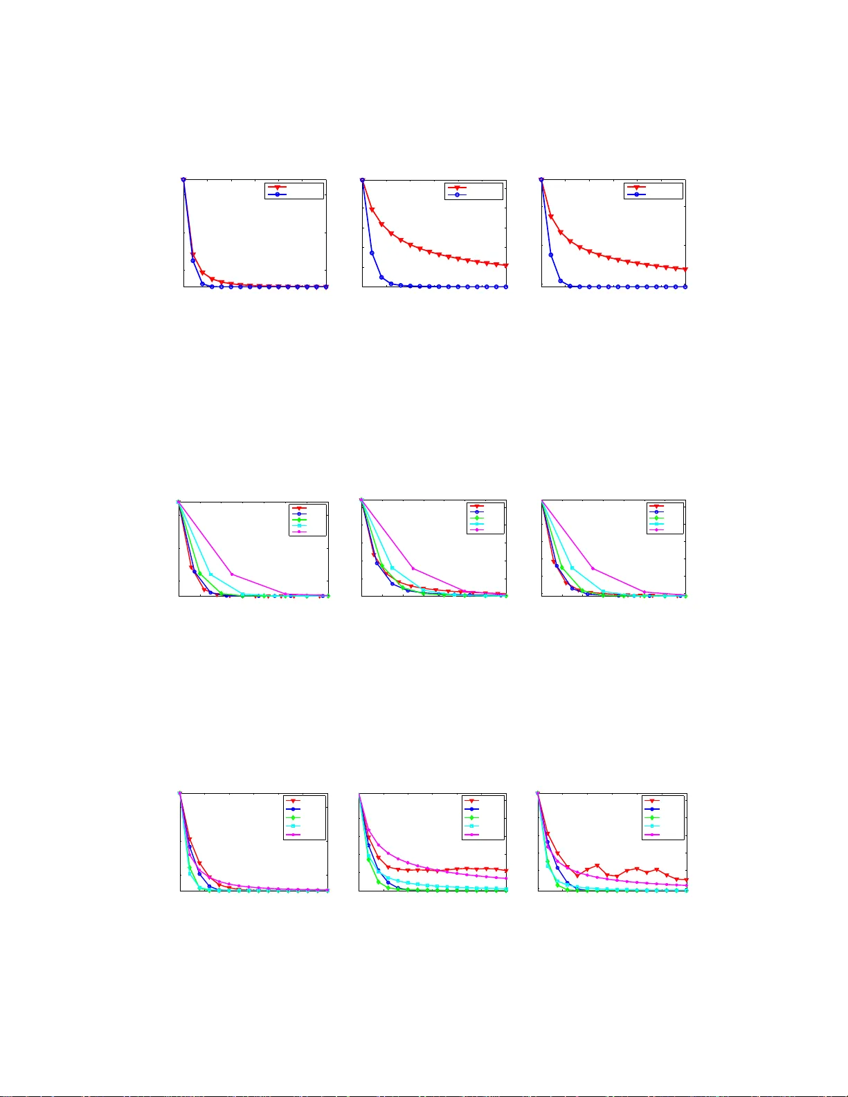
Linear Con vergence of V ariance-R educed Stochast ic Gradient without Str ong Con vexity Pinghua Gong, Jieping Y e Departmen t of Computation al Medicine and Bioinformatics University of Michigan, MI 4810 9 gongp @umich.edu , jpye@umich.edu Abstract Stochastic gradient algo rithms estimate the gradien t based on only one or a few samples and enjoy low computatio nal co st per iteration. They hav e been widely used in large-scale optimization problems. Ho wever , sto chastic gradient algo- rithms are usually slow to converge and ach ie ve sub-linear convergence rates, due to the in herent variance in th e gradien t compu tation. T o accelerate th e con- vergence, some variance-red uced stochastic gradient algor ithms, e.g., prox imal stochastic variance-redu ced gr adient (Prox-SVRG) algorithm , ha ve recen tly been propo sed to solve stro ngly co n vex problem s. Under th e stron gly conve x co ndi- tion, these variance-red uced stochastic gr adient algo rithms achieve a linear con- vergence rate. Howe ver , many machine learning problems are con vex but not strongly conv ex. In this pap er , we introduc e Prox -SVRG and its projected v ar iant called V ariance-Reduced Projected Stochastic Gradient (VRPSG) to so lve a class of non-stro ngly co n vex optimization p roblems widely used in mach ine learning. As the main technical con tribution of this p aper , we show that both VRPSG an d Prox-SVRG achieve a linear convergence rate without stron g co n vexity . A key ingredien t in our proo f is a Semi-Strong ly Conv ex (SSC) inequa lity which is th e first to be r igorou sly proved f or a class of non- strongly c on vex problems in bo th constrained and re g ularized settings. Moreover , the SSC inequality is indep endent of algorithms and may be app lied to analyze other stochastic g radient algo rithms besides VRPSG and Prox -SVRG, which m ay be of in depend ent inter est. T o the best of o ur kno wledge, this is the first work that establishes the linear co n ver- gence r ate fo r th e variance-red uced stochastic grad ient algor ithms on s olving both constrained and regularized problems without strong con vexity . 1 Intr oduction Con vex op timization h as p layed an importan t role in mach ine lear ning as many mach ine lea rning problem s can be cast in to a con vex optimization pr oblem. Now a days the em ergence of b ig data makes the o ptimization problem ch allenging to so lve an d first-o rder stocha stic g radient algorithms are often pref erred due to their simplicity and low per-iteration cost. The stochastic gradient algo- rithms estimate the gr adient based on only one or a few samples, and have b een extensi vely studied in large-scale optimization prob lems [27, 4, 7, 24, 5, 1 6, 1 0, 19]. In general, the stan dard stochas- tic gr adient algorithm r andomly dr aws o nly on e or a few samples a t e ach iteration to com pute the gradient and then update the m odel parameter . The standard stochastic gradient alg orithm estimates the g radient w ithout in volving all s amples and the computation al cost per iteration is independen t of the sample size. Thus, it is very suitable for large-scale pro blems. Howe ver, the standard stoch astic gradient algor ithms usu ally suffer from s low conver gence. In pa rticular , ev en unde r the stro ngly conv ex condition , the con vergen ce rate of standard stochastic gradient alg orithms is on ly su b-linear . In contrast, it is well-known that full gradient descent a lgorithms can achieve linear co n vergence 1 rates with the strongly co n vex condition [14]. It has b een recogn ized that the slow co n vergenc e of the standar d stochastic gr adient algorith m results fro m the inheren t v ariance in the gr adient ev alu- ation. T o this end, some (imp licit or explicit) variance-redu ced s tochastic g radient alg orithms have been p roposed rec ently; exam ples include Stochastic A verage Gradient (SA G) [1 1], Stoch astic Dua l Coordinate Ascent (SDCA) [17, 18], Epoch Mixed Grad ient Descent (EMGD) [26], S tochastic V ari- ance Reduced Gradie nt (SVRG) [ 8], Semi-Sto chastic Gra dient Descent (S2GD) [9] an d Proxim al Stochastic V ariance Red uced Gradien t (Prox-SVRG) [25]. Under the stro ngly conve x co ndition, these variance-r educed stochastic gradient algorith ms achiev e linear con vergence rates. Howe ver , in practical prob lems, many objective functio ns to be min imized ar e conve x but not stron gly co n vex. For example, the least sq uares r egression and logistic r egression prob lems are extensiv ely studied and both objective functions are not strongly conv ex when the data matrix is n ot full column rank. Moreover , e ven witho ut the strongly conv ex con dition, linear conver gence rates can be ach iev e d for som e fu ll gradient descent alg orithms [1 3, 12, 22, 2 1, 6, 23]. This m otiv ates us to addr ess the following question: can some variance-red uced stoch astic gradient algorithms achiev e a linear con- vergence r ate under mild conditions b u t without strong con vexity? In this p aper, we adop t Pro x-SVRG [ 25] and i ts projected variant called V ariance-Redu ced Projected Stochastic Grad ient (VRPSG) to solve a class of no n-strong ly conve x optimization proble ms. Ou r major techn ical contribution is to establish a linear co n vergenc e rate for b oth VRPSG and Prox- SVRG withou t stro ng convexity . The key challeng e to p rove the linear co n vergence for bo th VRPSG and Prox-SVRG lies in h ow to establish a Semi-Stron gly Conve x (SSC) in equality whic h pr ovides an up per bo und of the distance o f any fea sible solu tion to the optim al solu tion set by the g ap betwee n the objec ti ve function value a t that feasible solution and the optimal objective fun ction value. The SSC inequality can b e easily established under th e condition th at the objectiv e fu nction is stron gly conv ex. Ho wever , it is n ot the case without the stron gly con vex c ondition. T o the best of our knowledge, we are the first to rigorously prove th e SSC inequality fo r a class of n on-strong ly convex problem s in both co nstrained and r egularized setting s. Mor eover , the SSC ineq uality may b e ap plied to analyze other stochastic gradient alg orithms besides VRPSG a nd Pr ox-SVRG, w hich may be of indepen dent interest (see Remark 3 in Section 3 .1). No te that e x isting conv ergence analyses fo r full g radient metho ds [13, 1 2, 22, 21, 6, 2 3] cann ot be directly extended to the stoch astic setting as they rely on a different inequality inv o lving fu ll gradient. Thus, it is nontrivial to establish the linear conv e rgence rate for the variance-reduced stochastic gradien t algorith ms on solving both constrained and regularized problems without strong con vexity . 2 Linear Con vergen ce of VRPSG and Prox-SVRG W e first p resent both co nstrained and regular ized o ptimization prob lems 1 , discuss some mild as- sumptions about the problems and sho w some examples th at satisfy the as sumptions. Then we present th e Semi-Str ongly Conve x (SSC) inequality and introduce VRPSG and Prox -SVRG to solve the optim ization prob lems. Finally , we state our main resu lts on li near co n vergence for both VRPSG and Prox-SVRG algorithms. The proof s are deferred to the following section . 2.1 Optimization Problems, Assu mptions and Examples Constrained Problems : W e first co nsider the following co nstrained optimization problem: min w ∈W  f ( w ) = h ( X w ) + q T w  , where w , q ∈ R d , X ∈ R n × d , (1) and make the following assump tions on the above prob lem: A1 f ( w ) is the average of n conv ex com ponents f i ( w ) , that is, f ( w ) = 1 n P n i =1 f i ( w ) , where ∇ f ( w ) and ∇ f i ( w ) are Lipsch itz continuous with constants L and L i , respectively . A2 T he e ffecti ve domain dom ( h ) o f h is open an d n on-emp ty . Moreover , h ( u ) is continuously differentiable on dom ( h ) and strongly con vex on any convex compact subset of dom( h ) . A3 T he constra int set W is a p olyhed ral set, e.g. W =  w ∈ R d : C w ≤ b  for some C ∈ R l × d , b ∈ R l . Mo reover , th e optimal solution set W ⋆ c to Eq. (1) is non-e mpty . 1 W e p r esent con st rained and regularized p roblems sepa rately , ho weve r the ana lysis of re gularized problems depends on some ke y results established for constrained problems. 2 Remark 1 Assump tion A2 in dicates that h ( u ) may n ot be str ongly conve x on do m( h ) but strictly conve x on dom( h ) . Notice that f ( · ) is conve x, so W ⋆ c must be conve x and the Eu clidean pr ojection of any w ∈ R d onto W ⋆ c is unique. Mor eover , for any finite w , u ∈ W , X w and X u must belon g to a conve x compact subset U ⊆ dom( h ) . Thus, by assumption A2 , ther e exists a µ > 0 such that h ( X w ) ≥ h ( X u ) + ∇ h ( X u ) T ( X w − X u ) + µ 2 k X w − X u k 2 , ∀ X w , X u ∈ U . Example 1 (Co nstrained Problems) : Ther e are many examples that satisfy a ssumptions A1-A3 , including three popular p roblems: ℓ 1 -constraine d least squares (i.e., Lasso [20]), ℓ 1 -constraine d logistic regression and the du al pr oblem of linear SVM. Sp ecifically , for t he ℓ 1 -constraine d least squares: the objectiv e f unction is f ( w ) = 1 2 n k X w − y k 2 ; th e con vex compo nent is f i ( w ) = 1 2 ( x T i w − y i ) 2 , where x T i is the i -th row of X ; the stro ngly conve x fu nction is h ( u ) = 1 2 n k u − y k 2 ; th e p olyhedr al set is W = { w : k w k 1 ≤ τ } = { w : C w ≤ b } , where each row of C ∈ R 2 d × d is a d -tup les of th e form [ ± 1 , · · · , ± 1] , and each entry of b ∈ R 2 d is τ . For the ℓ 1 - constrained logistic regression: the obje cti ve fun ction i s f ( w ) = 1 n P n i =1 log(1 + exp( − y i x T i w )) ; the conv ex com ponent is f i ( w ) = log(1 +exp( − y i x T i w )) , where X = [ x T 1 ; · · · ; x T n ] T ; the stron gly conv ex function 2 is h ( u ) = 1 n P n i =1 log(1 + exp( − y i u i )) ; the polyh edral set is the same as the ℓ 1 - constrained lea st sq uares. For th e d ual p roblem o f line ar SVM, the objective is a conv ex quadratic function wh ich satisfies assump tions A1-A2 ; the constraint set is W = { w : l i ≤ w i ≤ u i } with l i ≤ u i ( i = 1 , · · · , d ) , which satisfies th e assump tion A3 . Additional constraint sets that satisfy the assump tion A 3 also include ℓ 1 , ∞ -ball set W = { w : P T i =1 k w G i k ∞ ≤ τ } with ∪ T i =1 G i = { 1 , · · · , d } and G i ∩ G j = ∅ f or i 6 = j [15]. Regularized Problems : Now let us consider the follo win g regularized o ptimization problem: min w ∈ R d { F ( w ) = f ( w ) + r ( w ) = h ( X w ) + r ( w ) } , w here X ∈ R n × d , (2) and we make the following ad ditional assumption besides assumptions A1, A2 : B1 r ( w ) is conv ex; th e epigraph of r ( w ) d efined by { ( w ,  ) : r ( w ) ≤  } is a polyhed ral set and the optimal solution set W ⋆ r to Eq. (2) is non-e mpty . Example 2 (Regularized Pr o blems) : Examples that satis fy assumptions A1, A2 and B 1 in clude ℓ 1 ( ℓ 1 , ∞ )-regularized least squares and logistic regression problems. 2.2 Semi-Strongly Con vex (SSC) Problem and Inequality Let us now introduce t he Semi-Strong ly Conve x ( SSC) proper ty . Definition 1 The pr o blem in Eq. ( 1) is SSC if the r e exists a constan t β > 0 such that fo r any finite w ∈ W : f ( w ) − f ⋆ ≥ β 2   w − Π W ⋆ c ( w )   2 , wher e f ⋆ is the optimal objective function value of Eq. (1) . The pr oblem in Eq. (2) is SSC if for an y finite w ∈ R d , ther e e xists a co nstant β > 0 such that F ( w ) − F ⋆ ≥ β 2   w − Π W ⋆ r ( w )   2 , wher e F ⋆ is the optimal objective function value of Eq. (2) . In Section 3 .1, we will rig orously prove that the p roblem in Eq. (1) is SSC un der assumptions A1-A3 and the pr oblem in Eq. (2) is SSC u nder assum ptions A1, A2 and B1 , wh ich is a key to show the linear con vergence o f VRPSG and Prox-SVRG to be gi ven belo w . T o t he best of our kno wledge, we are the first to provid e a rigor ous p roof of the SSC in equality for bo th co nstrained and regularized problem s in Eq. (1) and Eq. (2) without strong conve x ity . Moreover , the SSC inequality may be of indep endent interest, as it m ay be applied to an alyze o ther stochastic gradien t algo rithms (see Remark 3 in Section 3.1). 2 The function h ( u ) = 1 n P n i =1 log(1 + exp( − y i u i )) is strictly con vex on R n and strongly con vex on any con vex comp act subset of R n . 3 2.3 Algorithms and Main Results VRPSG for solving Eq. (1) : A standa rd stoch astic method for solving Eq. ( 1) is th e pro jected stochastic gradient algorithm which generates the sequence { w k } as follows: w k = Π W ( w k − 1 − η k ∇ f i k ( w k − 1 )) , (3) where i k is random ly drawn from { 1 , · · · , n } in un iform. At each iteration, the projected stochastic gradient alg orithm compu tes th e grad ient inv olving only a sing le sample an d thus is suitable for large-scale p roblems with large n . Althou gh we have an unb iased g radient estimate at each step, i.e., E  ∇ f i k ( w k − 1 )  = ∇ f ( w k − 1 ) , th e variance E  k∇ f i k ( w k − 1 ) − ∇ f ( w k − 1 ) k 2  introdu ced by sampling makes the step size η k diminishing to gu arantee c on vergen ce, which finally results in slow conver g ence. Ther efore, th e key fo r imp roving the conv ergence rate of the projected stoc has- tic g radient algo rithm is to reduce the variance b y samplin g. Motiv ated b y the variance-redu ce technique s in [8, 2 5], we co nsider a pr ojected variant of Prox -SVRG [25] called V arianc e-Reduced Projected Stochastic Gradien t (VRPSG) (in Algorithm 1) to efficiently solve Eq. ( 1) [i.e., VRPSG is equiv a lent to Pr ox-SVRG b y u sing a pr oximal step instead of th e p rojection step in Algorithm 1 (Line 10)]. Both VRPSG and Pro x-SVRG employ a two-layer lo op to r educe th e v ariance. W e have the following con vergence result: Algorithm 1: VRPSG: V ariance-Reduced Projected Stochastic Gradient 1 Cho ose the update frequency m a nd the learning rate η ; 2 In itialize ˜ w 0 ∈ W ; 3 Cho ose p i ∈ (0 , 1) such th at P n i =1 p i = 1 ; 4 for k = 1 , 2 , · · · do 5 ˜ ξ k − 1 = ∇ f ( ˜ w k − 1 ) ; 6 w k 0 = ˜ w k − 1 ; 7 for t = 1 , 2 , · · · , m do 8 Randomly pick i k t ∈ { 1 , · · · , n } according to P = { p 1 , , · · · , p n } ; 9 v k t = ( ∇ f i k t ( w k t − 1 ) − ∇ f i k t ( ˜ w k − 1 )) / ( np i k t ) + ˜ ξ k − 1 ; 10 w k t = Π W ( w k t − 1 − η v k t ) = ar g min w ∈W 1 2 k w − ( w k t − 1 − η v k t ) k 2 ; 11 end 12 ˜ w k = 1 m P m t =1 w k t ; 13 end Theorem 1 Let w ⋆ ∈ W ⋆ c be any optimal so lution to Eq. (1), f ⋆ = f ( w ⋆ ) be the optimal objective function valu e in E q. (1) and L P = max i ∈{ 1 , ··· ,n } [ L i / ( np i )] with p i ∈ (0 , 1) , P n i =1 p i = 1 . In addition , let 0 < η < 1 / (4 L P ) and β = 1 θ 2  1+2 k∇ h ( r ⋆ ) k 2 µ + M  , (4) wher e θ > 0 is a co nstant whose estimate is pr ovided in Lemma 7 a nd Rema rk 4 in S upplement B; µ > 0 is the s tr ongly con vex mod ulus of h ( · ) in some con vex co mpact set; M > 0 is an up per bou nd of f ( w ) − f ⋆ for any w ∈ W ; r ⋆ is a constan t vector such that X w ⋆ = r ⋆ for all w ⋆ ∈ W ⋆ c (r efer to Lemma 5 in Supplemen t B fo r mor e details abo ut r ⋆ ). I f m is su fficiently l ar ge such that ρ = 4 L P η ( m + 1) (1 − 4 L P η ) m + 1 β η (1 − 4 L P η ) m < 1 , (5) then under the assumption that { w k t } is bound ed a nd A1 − A3 ho ld, th e VRPSG algo rithm (su mma- rized in Algorithm 1) achieves a linear con ver gence r a te in expectation: E F k m  f ( ˜ w k ) − f ⋆  ≤ ρ k ( f ( ˜ w 0 ) − f ⋆ ) , wher e ˜ w k is defined in Algorithm 1 and E F k m [ · ] denotes the expectation with r espect to th e random variab le F k m with F k t (1 ≤ t ≤ m ) being defi ned as F k t = { i 1 1 , · · · , i 1 m , i 2 1 , · · · , i 2 m , · · · , i k − 1 1 , · · · , i k − 1 m , i k 1 , · · · , i k t } an d F k 0 = F k − 1 m , wh er e i k t is the sam - pling random variable in Algorithm 1. 4 Note that th e linea r co n vergence r ate ρ in Eq. ( 5) is the same with th at of Prox-SVRG in [25], except that the con stant β > 0 is slightly more complicated . Th is is expected since o ur co n vergence analysis does no t r equire the stro ngly conve x co ndition. I nterested reader s ma y refer to Supplemen t A and [25] for more details abou t th e above linear convergence. Prox-SVRG for solving Eq. (2) : W e use Prox-SVRG to solve Eq. (2) [i.e., u sing A lgorithm 1 to solve the regularize d pr oblem in Eq. (2) b y r eplacing the p rojection step in Algorith m 1 (Line 10 ) with the following p roximal step]: w k t = ar g min w  1 2 η   w − ( w k t − 1 − η v k t )   2 + r ( w )  . (6) Next we show tha t the con vergence analy sis in Theorem 1 can be accordingly extended t o the regu- larized setting; the main result is summarized in the following t heorem: Theorem 2 Let assump tions A1, A2 an d B1 h old. If we ad opt Pr ox-SVR G to solve the re gularized pr oblem in Eq. (2) [i.e., using Alg orithm 1 by replacing the pr ojection step in Algorithm 1 (Line 10) with the p r oximal step in E q. ( 6)] and a ssume that { w k t } is boun ded, then Theo r em 1 still h olds by r epla cing Eq. (1) and f ( · ) with Eq. (2) and F ( · ) , r espe ctively . 3 T ech nical Proof The key to p rove th e line ar conv e rgence results is to establish the Semi-Stro ngly Conve x ( SSC) inequality in Definition 1. No te that the SSC in equality does not in volve full gradient and is suitab le to prove linear con vergence of sto chastic gradient algorith ms. W e want to emphasize that the linear conv e rgence analysis fo r fu ll grad ient me thods [13, 12, 22, 21, 6, 23] r ely o n a different in equality k w − Π W ⋆ c ( w ) k ≤ κ k w − Π W ⋆ c ( w − ∇ f ( w )) k in volving fu ll g radient and cann ot be directly applied h ere. It is well-kn own that the SSC ineq uality ho lds under the strongly conve x co ndition. Howe ver, without the strongly conve x conditio n, it is n on-trivial to o btain this inequ ality . W e also note th at the SSC ineq uality ho lds deter ministically for all examples listed in Sectio n 2 .1, th us it is significantly dif f erent from the restricted st rong conv exity (RSC) in [1], where RSC hold s with high probab ility wh en the design matrix is sampled from a certain distribution. 3.1 Proof of the SSC Inequality in Constrained and Regularized Settings W e first p rove the SSC ineq uality (in Lemm a 1) f or the pr oblem in E q. (1) und er assumptio ns A1 - A3 . Then based o n the key results in th e proof of Le mma 1, we p rove th e SSC inequ ality (in Lemma 2) for th e p roblem in Eq . (2) und er assumption s A1, A2 and B1 , which is a no n-trivial extension (see Remark 2 for more details). Lemma 1 (SSC in equality for con strained pr ob lems) Und er assumption s A1 - A3 , th e p r oblem in Eq. (1) satisfies the SSC inequality with β > 0 defin ed in Eq. (4). Proof Let ¯ w = Π W ⋆ c ( w ) . If w ∈ W ⋆ c , the n ¯ w = w and the in equality holds for any β > 0 . W e next prove th e ineq uality for w ∈ W , w / ∈ W ⋆ c . Acco rding to Lemma 5 (in Supple ment B), we know th at there exist unique r ⋆ and s ⋆ such that W ⋆ c = { w ⋆ : C w ⋆ ≤ b , X w ⋆ = r ⋆ , q T w ⋆ = s ⋆ } which is non-e mpty . For any w ∈ W = { w : C w ≤ b } , the Eu clidean projection of C w − b o nto the non -negativ e orthant, deno ted by [ C w − b ] + , is 0 . Consider ing L emma 7 (in Supplemen t B) , for w ∈ W = { w : C w ≤ b } , there exist a w ⋆ ∈ W ⋆ c and a constan t θ > 0 such that k w − ¯ w k 2 ≤ k w − w ⋆ k 2 ≤ θ 2 ( k X w − r ⋆ k 2 + ( q T w − s ⋆ ) 2 ) , (7) where the first ineq uality is due to ¯ w = Π W ⋆ c ( w ) and w ⋆ ∈ W ⋆ c . By assum ption A3 , we know that W is co mpact. Th us, f or any finite w ∈ W , both X w and X ¯ w belo ng to so me co n vex com pact subset U ⊆ R n . Moreover , we ha ve X ¯ w = r ⋆ . Thu s, by the stron g conv exity of h ( · ) o n the subset U , ther e e x ists a constant µ > 0 such that h ( X w ) − h ( X ¯ w ) ≥ ∇ h ( X ¯ w ) T ( X w − X ¯ w ) + µ 2 k X w − r ⋆ k 2 , which together with f ( w ) = h ( X w ) + q T w implies that f ( w ) − f ( ¯ w ) ≥ ∇ f ( ¯ w ) T ( w − ¯ w ) + µ 2 k X w − r ⋆ k 2 . (8) 5 Noticing that w ∈ W and ¯ w ∈ W ⋆ c , we have ∇ f ( ¯ w ) T ( w − ¯ w ) ≥ 0 , which together with Eq. (8) implies that 2 µ ( f ( w ) − f ( ¯ w )) ≥ k X w − r ⋆ k 2 . (9) Next we establish the relation ship between ( q T w − s ⋆ ) 2 and f ( w ) − f ⋆ . W e kn ow that q = ∇ f ( ¯ w ) − X T ∇ h ( r ⋆ ) and s ⋆ = q T ¯ w by Lemma 5 (in Supplem ent B), we kno w that q T w − s ⋆ = q T ( w − ¯ w ) = ( ∇ f ( ¯ w ) − X T ∇ h ( r ⋆ )) T ( w − ¯ w ) = ∇ f ( ¯ w ) T ( w − ¯ w ) − ∇ h ( r ⋆ ) T ( X w − r ⋆ ) , which implies that ( q T w − s ⋆ ) 2 = ( ∇ f ( ¯ w ) T ( w − ¯ w ) − ∇ h ( r ⋆ ) T ( X w − r ⋆ )) 2 ≤ 2( ∇ f ( ¯ w ) T ( w − ¯ w )) 2 + 2 ( ∇ h ( r ⋆ ) T ( X w − r ⋆ )) 2 , which together with 0 ≤ ∇ f ( ¯ w ) T ( w − ¯ w ) ≤ f ( w ) − f ⋆ implies that ( q T w − s ⋆ ) 2 ≤ 2( f ( w ) − f ⋆ ) 2 + 2 k∇ h ( r ⋆ ) k 2 k X w − r ⋆ k 2 . (10) Substituting Eqs. ( 9), (10) into Eq. (7), we hav e k w − ¯ w k 2 ≤ 2 θ 2  1 + 2 k∇ h ( r ⋆ ) k 2 µ ( f ( w ) − f ⋆ ) + ( f ( w ) − f ⋆ ) 2  , which together with f ( w ) − f ⋆ ≤ M (L emma 6 in Supplement B) implies that k w − ¯ w k 2 ≤ 2 θ 2  1 + 2 k∇ h ( r ⋆ ) k 2 µ + M  ( f ( w ) − f ⋆ ) . This completes the proof of the lemma by considering the definition of β in Eq . (4).  Remark 2 Du e to the p r ojection step in Algorithm 1 (Line 10), ea ch iterate belon gs to the c onstraint set W . Mo r eover , the optimal solution set W ⋆ c is an intersection of the polyhe dral set W and an affine space { w ⋆ : X w ⋆ = r ⋆ , q T w ⋆ = s ⋆ } . The above fact is critical to pr ove the SS C i nequa lity for the constrained p r oblem in Eq. (1). However , for the r egularized pr o blem in Eq. (2), n o such p r operty holds. Thus it is much mo r e challeng ing to extend the SS C inequ ality to the r egularized pr o blem. Inter e stingly , we fin d that that the pr oblem in E q. (2) is equiva lent to the following co nstrained pr oblem (the pr o of is pr ovided in Lemma 8 in Supplement B): min ( w , ) ∈ f W n e F ( w ,  ) = f ( w ) +  = h ( X w ) +  o , wher e f W = { ( w ,  ) : r ( w ) ≤  } . (11) Based on the above equivalence and some ke y r esults in the pr oo f of Lemma 1, we establish an SSC inequality for th e r egularized pr oblem. Note th at we still solve the r e gu larized pr ob lem in Eq. (2) using Pr ox-S VRG and Eq. (11 ) is only used to pr ove the SSC inequality below . Lemma 2 (SSC inequa lity for r e g ularized pr oblems) U nder assumptions A1, A2 a nd B1 , the pr ob- lem in Eq. (2) satisfies the SSC inequality with β > 0 defin ed 3 in Eq. (4). Proof By Lemma 8 (in Supp lement B ) , the optimal solution sets to Eq. (2) and Eq. (11) are W ⋆ r = { w ⋆ : X w ⋆ = ˜ r ⋆ , r ( w ⋆ ) = ˜ s ⋆ } (12) and f W ⋆ = { ( w ⋆ ,  ⋆ ) : X w ⋆ = ˜ r ⋆ , r ( w ⋆ ) ≤  ⋆ = ˜ s ⋆ } (13) = { ( w ⋆ ,  ⋆ ) : X w ⋆ = ˜ r ⋆ , r ( w ⋆ ) =  ⋆ = ˜ s ⋆ } , (14) 3 β still has the same form as in Eq. (4), where each v ariable is accordingly cha nged from Eq. (1 ) to Eq. (11). 6 where ˜ r ⋆ and ˜ s ⋆ are constants. By Eqs. (2), (11), for any ( w ,  ) satisfy ing r ( w ) =  , we hav e F ( w ) − F ⋆ = e F ( w ,  ) − e F ⋆ , where e F ⋆ is the optimal objective fu nction v alue of Eq . (11) . Considering Eqs. (12), (14) together, we have Π f W ⋆ (( w ,  )) = (Π W ⋆ r ( w ) , ˜ s ⋆ ) . Notice that f W ⋆ in Eq . (13) is an in tersection of a polyhe dral set { ( w ⋆ ,  ⋆ ) : r ( w ⋆ ) ≤  ⋆ } and an affine s pace { ( w ⋆ ,  ⋆ ) : X w ⋆ = ˜ r ⋆ ,  ⋆ = ˜ s ⋆ } . Thu s, ( w ,  ) ∈ { ( w ,  ) : r ( w ) ≤  } fo r any w with r ( w ) =  . Using a similar proo f of Lem ma 1, we ha ve for any finite w satisfy ing r ( w ) =  : F ( w ) − F ⋆ = e F ( w ,  ) − e F ⋆ ≥ β 2   ( w ,  ) − Π f W ⋆ (( w ,  ))   2 = β 2   ( w ,  ) − (Π W ⋆ r ( w ) , ˜ s ⋆ )   2 ≥ β 2 k w − Π W ⋆ r ( w ) k 2 . This completes the proof of the lemma.  Remark 3 The SSC inequa lity for bo th constrained and re gularized p r oblems is in depend ent of algorithms. Thus, the SS C inequality may be of indep endent inter est. In p articular , any algo rithm whose linear con ver gence pr oof depends on f ( w ) − f ⋆ ≥ µ k w − w ⋆ k 2 ( µ > 0 ) can po tentially be adapted to solve the no n-str ongly con vex pr ob lems in Eqs. (1), (2) and achieve a linear co n v er gence rate using the SSC inequality . 3.2 Proof S ketch of Theorem 1 and Theorem 2 Once w e obta in the SSC in equality ab ove, the pro ofs of T heorem 1 and Th eorem 2 can be ad apted from [25] (The key d ifference is that we o btain th e SSC inequality withou t the strong co n vexity). Due to the space limit, w e only provide a pro of s ketch of Theor em 1 an d the d etailed proofs of b oth theorems are provided in Supplement C. Outline of the Proof of Th eorem 1 Let ¯ w k t = Π W ⋆ c ( w k t ) for all k , t ≥ 0 . The n we have ¯ w k t − 1 ∈ W ⋆ c , which together with the definition of ¯ w k t and g k t = ( w k t − 1 − w k t ) /η im plies that   w k t − ¯ w k t   2 ≤   w k t − ¯ w k t − 1   2 =   w k t − 1 − η g k t − ¯ w k t − 1   2 . Thus, following the proof of Theorem 3.1 in [25], we obtain ( the detailed proof is in Supplement C) 2 η (1 − 4 L P η ) m X t =1 E F k m  f ( w k t ) − f ⋆  ≤ E F k − 1 m h   w k 0 − ¯ w k 0   2 i + 8 L P η 2 ( m + 1) E F k − 1 m  f ( ˜ w k − 1 ) − f ⋆  , ( 15) By the conv exity of f ( · ) , we have f ( ˜ w k ) = f  1 m P m t =1 w k t  ≤ 1 m P m t =1 f ( w k t ) . Thus, we have m  f ( ˜ w k ) − f ⋆  ≤ m X t =1  f ( w k t ) − f ⋆  , (16) Considering Lemma 1 with boun ded { ˜ w k − 1 } , ˜ w k − 1 = w k 0 ∈ W and ¯ w k 0 = Π W ⋆ c ( w k 0 ) , we hav e f ( ˜ w k − 1 ) − f ⋆ = f ( w k 0 ) − f ⋆ ≥ β 2   w k 0 − ¯ w k 0   2 , which together with Eqs. (15), (16) implies that 2 η (1 − 4 L P η ) m E F k m  f ( ˜ w k ) − f ⋆  ≤  8 L P η 2 ( m + 1) + 2 β  E F k − 1 m  f ( ˜ w k − 1 ) − f ⋆  . Thus, we have E F k m  f ( ˜ w k ) − f ⋆  ≤  4 L P η ( m + 1) (1 − 4 L P η ) m + 1 β η (1 − 4 L P η ) m  E F k − 1 m  f ( ˜ w k − 1 ) − f ⋆  . By considerin g th e definition of ρ in Eq . (5), we complete the proof of the theorem.  7 4 Experiments Empirical resu lts in [25] have shown the effecti ven ess of Prox -SVRG on solv ing the regularize d problem . Thus, in this section, we ev alu ate the effecti veness of VRPSG by solving th e following ℓ 1 -constraine d lo gistic regression problem: min w ∈ R d ( f ( w ) = 1 n n X i =1 log(1 + exp( − y i x T i w )) , s.t. k w k 1 ≤ τ ) , where n is th e nu mber of samp les; τ > 0 is the c onstrained par ameter; x i ∈ R d is th e i -th sample; y i ∈ { 1 , − 1 } is the lab el of the sam ple x i . For the above problem , it is easy to obtain that the co n vex compon ent is f i ( w ) = log(1 + exp( − y i x T i w )) and the Lipschitz constan t of ∇ f i ( w ) is k x i k 2 / 4 . W e co nduct exper iments on three rea l-world data sets: c lassic ( n = 7 094 , d = 4 1681 ) , reviews ( n = 4069 , d = 184 82 ) and sports ( n = 8580 , d = 1486 6 ), which ar e sparse text data and ca n b e downloaded online 4 . W e co nduct comparison b y in cluding the fo llowing algorith ms (more experi- mental results are p rovided in the supp lementary m aterial d ue to space lim it): (1) AFG: the accel- erated fu ll grad ient algorith m proposed in [2] with an ad aptive line search. (2 ) SGD: th e stoch astic gradient descen t algorithm in Eq. (3). As sug gested by [4], we set the step size as η k = η 0 / √ k , where η 0 is an initial step size. (3) VRPSG: the variance-reduc ed projected stochastic grad ient al- gorithm in this paper . (4) VRPSG2: a hybrid algo rithm by executing SGD for one pass o ver the data and then switching to the VRPSG algorithm (similar schemes are also adopted in [8, 25]). 0 5 10 15 20 25 30 10 −10 10 −5 #grad/n Objective Function Value Gap classic VRPSG VRPSG2 SGD( η 0 =5) SGD( η 0 =1) SGD( η 0 =0.2) SGD( η 0 =0.04) AFG 0 5 10 15 20 25 30 10 −4 10 −3 10 −2 10 −1 10 0 #grad/n Objective Function Value Gap reviews 0 5 10 15 20 25 30 10 −8 10 −6 10 −4 10 −2 10 0 #grad/n Objective Function Value Gap sports Figure 1: Comp arison of different algorithms: th e objective fun ction v alue gap f ( ˜ w k ) − f ⋆ vs. th e number of gradient e valuations ( ♯ grad/n) plots ( av e raged o n 10 runs). The parameter of VRPSG are set as τ = 1 0 , η = 1 /L P , m = n , p i = L i / P n i =1 L i ; the step size of SGD is set as η k = η 0 / √ k . Note that SGD is sensitive to the initial step si ze η 0 [4]. T o have a fair comparison of dif feren t algo- rithms, we set d ifferent values of η 0 for SGD to o btain th e b est p erforma nce ( η 0 = 5 , 1 , 0 . 2 , 0 . 04 ) . T o provide an implementatio n in depend ent result for all algorithms, we report th e o bjectiv e fu nction value ga p f ( ˜ w k ) − f ⋆ vs. the numb er o f grad ient ev aluatio ns 5 ( ♯ grad/n) plots in Figure 1 , f rom which we have the fo llowing observations: (a) Both stoch astic algorithm s (VRPSG and SGD with a pr oper initial step size) outperf orm the full gradien t algorithm (AFG). (b ) SGD quick ly decreases the objective function value in the beginn ing and g radually slows down in th e fo llowing iterations. In con trast, VRPSG decr eases the objective fun ction value linea rly fro m the beginn ing. This phe- nomeno n is comm only expected due to the sub-linea r con vergenc e rate of SGD and th e linear c on- vergence r ate of VRPSG. (c ) VRPSG2 p erforms slightly better than VRPSG, wh ich d emonstrates that the hyb rid sch eme can empir ically imp rove the perfo rmance. Similar results are also re ported in [8, 25]. 5 Conclusion In this paper, we study Prox-SVRG an d its projected variant VRPSG on efficiently solv ing a class of non-stro ngly con vex optimization p roblems in b oth constra ined and r egularized settings. Our main technical co ntribution is to estab lish a linear convergence analysis fo r both VRPSG and Prox-SVRG without strong con vexity . T o the best o f our kno wledge, th is is the first line ar con vergence result for variance-reduced stoch astic gradien t alg orithms on solving b oth con strained an d regularized prob- lems without the strongly conve x condition . In th e fu ture work, we will try to develop a more gen eral conv e rgence analy sis for a wide r range of p roblems includin g both non- polyhed ral co nstrained and regularized optimization problems. 4 http://www.shi- zhong.co m/software/docdata .zip 5 Computing the gradient on a single sample counts as one gradient ev aluation. 8 Refer ences [1] A. Agarwal, S. Negah ban, and J. W ainwright. Fast global con ver gence of gradient methods for high- dimensional statistical recov ery . The Annals of Statistics , 40(5):2452–2 482, 2012. [2] A. Beck and M. T eboulle. A fast it erativ e shrinkage-thresholding algorithm for linear in verse problems. SIAM Jo urnal on Imag ing Sciences , 2(1):183–202, 2009. [3] D. Bertsekas. Nonlinear Pro gramming . A thena Scientific, 1999. [4] J. Duchi and Y . S inger . Efficient online and batch learning using forward backward splitting. Journa l of Mach ine Learning Resear ch , 10:28 99–293 4, 2009. [5] E. Hazan and S. Kale. B eyo nd the regret minimization barrier: an optimal algorithm for stochastic strongly-con ve x optimization. Jo urnal of Machine Learning Researc h-Proce edings T rack , 19:421–43 6, 2011. [6] K. Hou, Z. Zhou, A. S o, an d Z. Luo. On the linear con v ergenc e of the pro ximal gradient metho d f or trace norm regu larization. In NIPS , pages 710–718 , 2013. [7] C. Hu, J. Kwok, and W . Pan. Accelerated gradient methods for stochastic optimization and online learn- ing. In NIPS , volume 22, pages 781–7 89, 2009. [8] R. Johnson and T . Zhang. Accelerating st ochastic gradient descent using predicti ve v ariance r eduction. In NIPS , pages 315–323 , 2013. [9] J. K one ˇ cn ` y and P . Richt ´ arik. Semi-stochastic gradient descent metho ds. arXiv pr eprint arXiv:1312.1666 , 2013. [10] G. Lan. An optimal method for stochastic composite optimization. Mathematical Pro gramming , 133(1- 2):365–39 7, 2012. [11] N. L e Roux, M. Schmidt, and F . Bach. A stochastic gradient method with an expon ential con vergence rate for finite training sets. In NIPS , pages 2672–268 0, 2012. [12] Z . Luo and P . Tseng. Error bounds and con vergence analysis of feasible descent methods: a general approach. Annals of Operations Resear ch , 46(1):157–178 , 1993. [13] Z .-Q. Luo and P . Tseng. On the con vergen ce of the coordinate descent method for con vex dif ferentiable minimization. Journ al of Optimization Theory and Applications , 72(1):7–35, 1992. [14] Y . Nesterov . Gradient methods for minimizing composite functions. M athematical P r ogra mming , 140(1):125– 161, 2013. [15] A. Q uattoni, X. Carreras, M. Collins, and T . Darrell. An ef ficient projection for ℓ 1 , ∞ regularization. In ICML , pages 857–864 , 2009. [16] A. Rakhlin, O. S hamir , and K. Sridharan. Making g radient desc ent optimal fo r strong l y con v ex stochastic optimization. arXiv pr eprint arXiv:1109.5647 , 2011. [17] S . Shalev-Shw art z and T . Zhang. Proximal stochastic dual coordinate ascent. arXiv pr eprint arXiv:1211.271 7 , 2012. [18] S . Shale v-Shwartz and T . Zhang. Stochastic dual coordina te ascent methods for re gularized loss. Jo urnal of Machine Learning Resear ch , 14(1):567–599, 2013. [19] O. Shamir and T . Zhang. Stochastic gradient descent for non-smooth optimization: Con vergenc e results and optimal av eraging schemes. In ICML , pages 71–79, 2013. [20] R . Tibshirani. Regression shrinkage and selection via the lasso. Journal of the Royal Statistical Society . Series B (Methodolo gical) , pages 267–288, 1996. [21] P . Tseng. Approximation accu racy , gradient metho ds, and err or bound f or structured con v ex optimization. Mathematical Pr ogramming , 125(2 ):263–295 , 2010. [22] P . Tseng and S . Y un. A coordinate gradient descent method for nonsmooth separable minimization. Mathematical Pr ogramming , 117(1 -2):387–42 3, 2009. [23] P . W ang and C. L in. Iteration complexity of feasible descent methods for con vex optimization. J ournal of Machine Learning Resear ch , 15:1523–1548 , 2014. [24] L . Xiao. Dual av eraging methods for regularized stochastic learning and online optimization. Journ al of Mach ine Learning Resear ch , 11(4):25 43–259 6, 2010. [25] L . Xiao and T . Zhang. A proximal stochastic g radient method with pro gressi ve varianc e reduction. SIAM J ournal on Optimization , 24:2057– 2075, 2014. [26] L . Zhang , M. Mahda vi, and R. Jin. Linear con ver gence with co ndition number independ ent access of full gradients. In NIPS , pages 980–988, 2013. [27] T . Zhang. Solving large scale linear prediction problems using stochastic gradien t descent algorithms. In ICML , 2004. 9 Supplemen tary Material for “Linear Con ver gence of V ariance-Reduced Stochastic Gradient without Str ong Con vexity” In this supplementary material, we first presen t some rem arks for Th eorem 1 in Su pplement A. Then we present some auxiliary Lem mas in Supplem ent B , wh ich will be used in the p roofs o f lin ear co n- vergence theorems in Supplemen t C. Fin ally we pr esent more exper imental resu lts in Supplement D. A Remarks for Theore m 1 W e have the follo win g remarks on the con vergence result in Th eorem 1: • L et η = γ / L P with 0 < γ < 1 / 4 . When m is sufficiently large, we have ρ ≈ L P /β γ (1 − 4 γ ) m + 4 γ 1 − 4 γ , where L P /β c an be treated as a p seudo conditio n number of the p roblem in Eq. (1) . If we choose γ = 0 . 1 and m = 100 L P /β , then ρ ≈ 5 / 6 . Notice that at each outer iteratio n of Algo rithm 1, n + 2 m gradien t evaluations (com puting the grad ient o n a sing le sample counts as one g radient ev a luation) are r equired. Th us, to obtain an ǫ -accuracy solution (i.e., E F k m  f ( ˜ w k ) − f ⋆  ≤ ǫ ), we need O ( n + L P /β ) lo g(1 /ǫ ) g radient evaluations by setting m = Θ( L P /β ) . In particular, the complexity be comes O ( n + L avg /β ) lo g(1 / ǫ ) if we cho ose p i = L i / P n i =1 L i for all i ∈ { 1 , · · · , n } , and O ( n + L max /β ) lo g(1 / ǫ ) if we c hoose p i = 1 /n for all i ∈ { 1 , · · · , n } , wher e L avg = P n i =1 L i /n a nd L max = max i ∈{ 1 , ··· ,n } L i . No tice that L avg ≤ L max . Th us, sam pling in proportio n to the Lip schitz constant is better than sampling uniform ly . • I f f is strongly conv ex with parameter ˜ µ and p i = L i / P n i =1 L i , VRPSG has the same complexity as Prox- SVRG [2 5], that is, VRPSG n eeds O ( n + L avg / ˜ µ ) log (1 /ǫ ) g radi- ent ev aluatio ns to obtain an ǫ -accuracy solutio n. In co ntrast, fu ll g radient metho ds and standard stochastic gradien t algor ithms with diminish ing step size η k = 1 / ( αk ) req uire O ( nL / ˜ µ ) log (1 /ǫ ) and O (1 / ( αǫ )) g radient ev aluatio ns to obtain a solution o f the same accuracy . O bviously , O ( n + L avg / ˜ µ ) log (1 /ǫ ) and is far sup erior over O ( nL/ ˜ µ ) log (1 /ǫ ) and O (1 / ( αǫ )) when the sample size n an d the condition number L/ ˜ µ are very large. • I f th e Lipschitz con stant L i is unkn own and d ifficult to compu te, we can u se an up per bou nd ˆ L i instead of L i to define L P = max i ∈{ 1 , ··· ,n } [ ˆ L i / ( np i )] and the theorem still holds. • W e can obtain a conver g ence rate with high pr obability . Accord ing to Markov’ s inequ ality with f ( ˜ w k ) − f ⋆ ≥ 0 , Theo rem 1 implies that Pr( f ( ˜ w k ) − f ⋆ ≥ ǫ ) ≤ E F k m  f ( ˜ w k ) − f ⋆  ǫ ≤ ρ k ( f ( ˜ w 0 ) − f ⋆ ) ǫ . Therefo re, w e ha ve Pr( f ( ˜ w k ) − f ⋆ ≤ ǫ ) ≥ 1 − δ , if k ≥ log  f ( ˜ w 0 ) − f ⋆ δǫ  / log(1 /ρ ) . B A uxiliary Lemmas Lemma 3 Let L and L i be the Lipschitz constants of ∇ f ( w ) an d ∇ f i ( w ) , respectively . Moreo ver , let L avg = P n i =1 L i /n , L max = max i ∈{ 1 , ··· ,n } L i and L P = max i ∈{ 1 , ··· ,n } [ L i / ( np i )] with p i ∈ (0 , 1) , P n i =1 p i = 1 . Th en we have L ≤ L avg ≤ L P and L avg ≤ L max . Proof Based on the defin ition of L ipschitz continu ity , we o btain tha t L and L i are the smallest positive constants such that for all w , u ∈ R d : k∇ f ( w ) − ∇ f ( u ) k ≤ L k w − u k , (17) k∇ f i ( w ) − ∇ f i ( u ) k ≤ L i k w − u k . (18) 10 Dividing Eq. (18 ) b y n and sum ming over i = 1 , · · · , n , we have 1 n n X i =1 k∇ f i ( w ) − ∇ f i ( u ) k ≤ 1 n n X i =1 L i k w − u k . (19) Based on the triangle inequality and ∇ f ( w ) = 1 n P n i =1 ∇ f i ( w ) we have k∇ f ( w ) − ∇ f ( u ) k ≤ 1 n n X i =1 k∇ f i ( w ) − ∇ f i ( u ) k , which together with L avg = P n i =1 L i /n a nd Eqs. (17), (1 9) implies that L ≤ L avg . Define s = [ L 1 /p 1 , · · · , L n /p n ] T . Noticing that L P = max i ∈{ 1 , ··· ,n } [ L i / ( np i )] with p i ∈ (0 , 1) , P n i =1 p i = 1 an d considering the definition of the dual norm, we ha ve nL P = max i ∈{ 1 , ··· ,n } L i p i = k s k ∞ = sup k t k 1 ≤ 1 t T s ≥ n X i =1 p i L i p i , which together with L avg = P n i =1 L i /n immed iately im plies that L avg ≤ L P . L avg ≤ L max is obvious by the definition of L avg = P n i =1 L i /n a nd L max = max i ∈{ 1 , ··· ,n } L i .  Lemma 4 Let w ⋆ ∈ W ⋆ c be an y optima l solution to th e pr ob lem in Eq. (1), f ⋆ = f ( w ⋆ ) be the op timal o bjective function valu e in Eq. (1) a nd L P = max i ∈{ 1 , ··· ,n } [ L i / ( np i )] with p i ∈ (0 , 1) , P n i =1 p i = 1 . Th en under assumptions A1 - A3 , for all w ∈ W , we ha ve 1 n n X i =1 1 np i k∇ f i ( w ) − ∇ f i ( w ⋆ ) k 2 ≤ 2 L P [ f ( w ) − f ⋆ ] . Proof For any i ∈ { 1 , · · · , n } , we consider the following fu nction φ i ( w ) = f i ( w ) − f i ( w ⋆ ) − ∇ f i ( w ⋆ ) T ( w − w ⋆ ) . It fo llows f rom the con vexity o f φ i ( w ) and ∇ φ i ( w ⋆ ) = 0 that min w ∈ R d φ i ( w ) = φ i ( w ⋆ ) = 0 . Recalling that ∇ φ i ( w ) = ∇ f i ( w ) − ∇ f i ( w ⋆ ) is L i -Lipschitz continuou s, we h av e for all w ∈ W : 0 = φ i ( w ⋆ ) ≤ min η ∈ R φ i ( w − η ∇ φ i ( w )) ≤ min η ∈ R  φ i ( w ) − η k∇ φ i ( w ) k 2 + L i η 2 2 k∇ φ i ( w ) k 2  = φ i ( w ) − 1 2 L i k∇ φ i ( w ) k 2 = φ i ( w ) − 1 2 L i k∇ f i ( w ) − ∇ f i ( w ⋆ ) k 2 , which implies for all w ∈ W : k∇ f i ( w ) − ∇ f i ( w ⋆ ) k 2 ≤ 2 L i φ i ( w ) = 2 L i ( f i ( w ) − f i ( w ⋆ ) − ∇ f i ( w ⋆ ) T ( w − w ⋆ )) . Dividing the a bove in equality by n 2 p i and summing over i = 1 , · · · , n , we have 1 n n X i =1 1 np i k∇ f i ( w ) − ∇ f i ( w ⋆ ) k 2 ≤ 2 L P ( f ( w ) − f ( w ⋆ ) − ∇ f ( w ⋆ ) T ( w − w ⋆ )) , (20) where we use L avg = P n i =1 L i /n ≤ L P = ma x i ∈{ 1 , ··· ,n } [ L i / ( np i )] (see Lemm a 3) and f ( w ) = 1 n P n i =1 f i ( w ) . Recalling that w ⋆ ∈ W ⋆ c is an o ptimal solution to E q. (1) and w ∈ W , it f ollows from the optimality condition of Eq. (1) that ∇ f ( w ⋆ ) T ( w − w ⋆ ) ≥ 0 , which together with Eq. (20) and f ⋆ = f ( w ⋆ ) immediately proves th e lemma.  Lemma 5 Under assumption s A1 - A3 , for all w ⋆ ∈ W ⋆ c , there exist uniqu e r ⋆ and s ⋆ such that X w ⋆ = r ⋆ and q T w ⋆ = s ⋆ . Moreover , W ⋆ c = { w ⋆ : C w ⋆ ≤ b , X w ⋆ = r ⋆ , q T w ⋆ = s ⋆ } . 11 Proof By assump tion A1 , we know that W ⋆ c is n ot empty . W e first p rove th at ther e exists a u nique r ⋆ such that X w ⋆ = r ⋆ by co ntradiction . Assume that there are w ⋆ 1 , w ⋆ 2 ∈ W ⋆ c such th at X w ⋆ 1 6 = X w ⋆ 2 . Then, the optimal objective function v alu e is f ⋆ = h ( X w ⋆ 1 ) + q T w ⋆ 1 = h ( X w ⋆ 2 ) + q T w ⋆ 2 . Due to w ⋆ 1 , w ⋆ 2 ∈ W ⋆ c and the conv exity of W ⋆ c , we have ( w ⋆ 1 + w ⋆ 2 ) / 2 ∈ W ⋆ c . Th erefore, f ⋆ = h  1 2 X w ⋆ 1 + 1 2 X w ⋆ 2  + 1 2 q T ( w ⋆ 1 + w ⋆ 2 ) . (21) On the other hand, the strong con vexity of h ( · ) implies that h  1 2 X w ⋆ 1 + 1 2 X w ⋆ 2  < 1 2 h ( X w ⋆ 1 ) + 1 2 h ( X w ⋆ 2 ) , which together with Eq. (21) implies that f ⋆ < 1 2 h ( X w ⋆ 1 ) + 1 2 h ( X w ⋆ 2 ) + 1 2 q T ( w ⋆ 1 + w ⋆ 2 ) = f ⋆ , leading to a contrad iction. Thus, ther e exists a uniqu e r ⋆ such that f or all w ⋆ ∈ W ⋆ c , X w ⋆ = r ⋆ . The uniqu eness of r ⋆ and f ⋆ immediately implies that ther e exists a u nique s ⋆ such that q T w ⋆ = s ⋆ . If w ⋆ ∈ W ⋆ c , then w ⋆ ∈ W , X w ⋆ = r ⋆ and q T w ⋆ = s ⋆ , that is, w ⋆ ∈ { w ⋆ : C w ⋆ ≤ b , X w ⋆ = r ⋆ , q T w ⋆ = s ⋆ } and h ence W ⋆ c ⊆ { w ⋆ : C w ⋆ ≤ b , X w ⋆ = r ⋆ , q T w ⋆ = s ⋆ } . If w ⋆ ∈ { w ⋆ : C w ⋆ ≤ b , X w ⋆ = r ⋆ , q T w ⋆ = s ⋆ } , th en w ⋆ is a feasib le solution and f ( w ⋆ ) = h ( X w ⋆ ) + q T w ⋆ = f ⋆ , that is, w ⋆ ∈ W ⋆ c and he nce { w ⋆ : C w ⋆ ≤ b , X w ⋆ = r ⋆ , q T w ⋆ = s ⋆ } ⊆ W ⋆ c . Therefo re, w e ha ve W ⋆ c = { w ⋆ : C w ⋆ ≤ b , X w ⋆ = r ⋆ , q T w ⋆ = s ⋆ } .  Lemma 6 Let w ∈ W = { w : X w ≤ b } an d f ⋆ be the o ptimal objective function valu e in Eq. (1). Then under assumptions A1 - A3 , for any finite w , there e xists a constan t M > 0 su ch that f ( w ) − f ⋆ ≤ M . Proof For any w ⋆ ∈ W ⋆ c , we have f ⋆ = f ( w ⋆ ) . Recalling that ∇ f ( w ) is Lipsch itz c ontinuou s with constant L , we hav e f ( w ) − f ⋆ ≤ ∇ f ( w ⋆ ) T ( w − w ⋆ ) + L 2 k w − w ⋆ k 2 , which together with Lemma 5 implies that there exists a constant v ector r ⋆ such that f ( w ) − f ⋆ ≤ ( X T ∇ h ( r ⋆ ) + q ) T ( w − w ⋆ ) + L 2 k w − w ⋆ k 2 ≤ k X T ∇ h ( r ⋆ ) + q kk w − w ⋆ k + L 2 k w − w ⋆ k 2 , Recall that k X T ∇ h ( r ⋆ ) + q k is constan t and both w and w ⋆ are finite. T hus, t he right-hand- side o f the above inequality must b e upper bo unded by a p ositi ve constant M . Th is comp letes the proof of the lemma.  Lemma 7 (Hoffman’s boun d, L emma 4.3 [23] ) Let V = { w : C w ≤ b , X w = r } be a non-empty polyhed r on. Then for a ny w ∈ R d , th er e exist a feasible poin t w ⋆ of V a nd a constan t θ > 0 such that k w − w ⋆ k ≤ θ     [ C w − b ] + X w − r     , wher e [ C w − b ] + denotes the Euclidea n pr ojectio n of C w − b onto the n on-negative orth ant and θ is the Hoffman constant defined by θ = sup u , v        u v     : k C T u + X T v k = 1 , u ≥ 0 the r ow s of C a nd X cor res ponding to the nonz ero components of u and v ar e l inear l y indep endent    < ∞ . Remark 4 Let D be a set inclu ding all matrices formed by the linearly independen t colu mns of the matrix [ C T , X T ] . The n for all D ∈ D , D T D is invertible and we have 0 < θ ≤ max D ∈D σ max (( D T D ) − 1 D T ) , wher e σ max ( · ) d enotes the maximum singular value . 12 Lemma 8 (a) Eq. (2) is eq uivalent to Eq. (11). Specifi cally , if w ⋆ is an op timal solution to Eq. (2) , then ( w ⋆ , r ( w ⋆ )) mu st b e an op timal solution to Eq. (11). If ( w ⋆ ,  ⋆ ) is an optimal solu tion to Eq. (1 1), then  ⋆ = r ( w ⋆ ) must ho ld a nd w ⋆ must be an op timal solu tion to Eq. (2). (b) There exis t constant ˜ r ⋆ and ˜ s ⋆ such that the optimal solu tion sets to Eq. (2) and Eq. (11) ar e W ⋆ r = { w ⋆ : X w ⋆ = ˜ r ⋆ , r ( w ⋆ ) = ˜ s ⋆ } and f W ⋆ = { ( w ⋆ ,  ⋆ ) : X w ⋆ = ˜ r ⋆ , r ( w ⋆ ) ≤  ⋆ = ˜ s ⋆ } = { ( w ⋆ ,  ⋆ ) : X w ⋆ = ˜ r ⋆ , r ( w ⋆ ) =  ⋆ = ˜ s ⋆ } . Proof (a) By the optimality condition of Eq. (2), w ⋆ is an optimal solution to Eq. (2), if and o nly if ∇ f ( w ⋆ ) T ( w − w ⋆ ) + r ( w ) − r ( w ⋆ ) ≥ 0 , ∀ w ∈ R d . (22) By the optimality condition of Eq. (11), ( w ⋆ ,  ⋆ ) is an optimal solution to Eq. (11), if and only if ∇ f ( w ⋆ ) T ( w − w ⋆ ) +  −  ⋆ ≥ 0 , ∀ w ,  su ch that r ( w ) ≤  . (23) If w ⋆ is an optima l solution to Eq. (2), then Eq . (22) immediately implies Eq. (2 3) by setting  ⋆ = r ( w ⋆ ) , i.e., ( w ⋆ , r ( w ⋆ )) must be an optima l solution to Eq. (11). If ( w ⋆ ,  ⋆ ) is an optimal solution to Eq . (11), let us assume that  ⋆ > r ( w ⋆ ) . T hen we h a ve e F ( w ⋆ ,  ⋆ ) > e F ( w ⋆ , r ( w ⋆ )) , which contradicts th e fact th at ( w ⋆ ,  ⋆ ) is an o ptimal so lution to Eq. (1 1). T herefor e,  ⋆ = r ( w ⋆ ) mu st hold. Moreover, Eq. (23) immediately implies Eq . (2 2) by setting and  = r ( w ) and con sidering that  ⋆ = r ( w ⋆ ) , i.e., w ⋆ must be an optimal solution to Eq. (2). (b) Recalling tha t r ( w ) is conve x , we can u se a similar argum ent of Lemm a 5 (in Supp lement B) to show that ther e exist constants ˜ r ⋆ 1 , ˜ r ⋆ 2 , ˜ s ⋆ 1 , ˜ s ⋆ 2 such that th e optim al solution sets to Eq . (2) and Eq. (1 1) are W ⋆ r = { w ⋆ : X w ⋆ = ˜ r ⋆ 1 , r ( w ⋆ ) = ˜ s ⋆ 1 } and f W ⋆ = { ( w ⋆ ,  ⋆ ) : X w ⋆ 2 = ˜ r ⋆ 2 , r ( w ⋆ ) ≤  ⋆ = ˜ s ⋆ 2 } . By the eq uiv alenc e in (a) , th ere exist ˜ r ⋆ and ˜ s ⋆ such that ˜ r ⋆ = ˜ r ⋆ 1 = ˜ r ⋆ 2 and ˜ s ⋆ = ˜ s ⋆ 1 = ˜ s ⋆ 2 . Next, we prove that { ( w ⋆ ,  ⋆ ) : X w ⋆ = ˜ r ⋆ , r ( w ⋆ ) ≤  ⋆ = ˜ s ⋆ } = { ( w ⋆ ,  ⋆ ) : X w ⋆ = ˜ r ⋆ , r ( w ⋆ ) =  ⋆ = ˜ s ⋆ } . T o show this, we o nly need to prove that { ( w ⋆ ,  ⋆ ) : X w ⋆ = ˜ r ⋆ , r ( w ⋆ ) ≤  ⋆ = ˜ s ⋆ } ⊆ { ( w ⋆ ,  ⋆ ) : X w ⋆ = ˜ r ⋆ , r ( w ⋆ ) =  ⋆ = ˜ s ⋆ } , since { ( w ⋆ ,  ⋆ ) : X w ⋆ = ˜ r ⋆ , r ( w ⋆ ) =  ⋆ = ˜ s ⋆ } ⊆ { ( w ⋆ ,  ⋆ ) : X w ⋆ = ˜ r ⋆ , r ( w ⋆ ) ≤  ⋆ = ˜ s ⋆ } hold s trivially . Let ( w ⋆ ,  ⋆ ) ∈ { ( w ⋆ ,  ⋆ ) : X w ⋆ = ˜ r ⋆ , r ( w ⋆ ) ≤  ⋆ = ˜ s ⋆ } , i.e., ( w ⋆ ,  ⋆ ) is an optimal solution to Eq. ( 11). Then , b y the con clusion in (a), we have r ( w ⋆ ) =  ⋆ = ˜ s ⋆ , which immediately implies that ( w ⋆ ,  ⋆ ) ∈ { ( w ⋆ ,  ⋆ ) : X w ⋆ = ˜ r ⋆ , r ( w ⋆ ) =  ⋆ = ˜ s ⋆ } . Therefo re, we have { ( w ⋆ ,  ⋆ ) : X w ⋆ = ˜ r ⋆ , r ( w ⋆ ) ≤  ⋆ = ˜ s ⋆ } ⊆ { ( w ⋆ ,  ⋆ ) : X w ⋆ = ˜ r ⋆ , r ( w ⋆ ) =  ⋆ = ˜ s ⋆ } .  C Proofs of Lin ear Con vergence Theor ems In ad dition to the SSC ineq ualities in Lemmas 1, 2, we also n eed the following two lemmas (Lem - mas 9 , 10) to prove the linear convergence theorems. Note that Lemma s 9, 1 0 are estab lished for constrained op timization pr oblems which are ad apted fro m Corollary 3.5 and Lemm a 3.7 f or regu- larized optimizatio n p roblems in [25]. The first lemma boun ds th e v ar iance of v k t in terms of the difference of objecti ve functions. Lemma 9 Let w ⋆ ∈ W ⋆ c be a ny optima l solution to the pr ob lem in E q. (1), f ⋆ = f ( w ⋆ ) be the optimal objective function value in Eq. (1). Then under assumptions A1 - A3 , we have E F k t  v k t | F k t − 1  = ∇ f ( w k t − 1 ) , (24) E F k t h   v k t − ∇ f ( w k t − 1 )   2 | F k t − 1 i ≤ 4 L P  f ( w k t − 1 ) − f ⋆ + f ( ˜ w k − 1 ) − f ⋆  , (25) wher e F k t is d efined in Th eor em 1; v k t , w k t − 1 , ˜ w k − 1 ar e define d in Algorithm 1 ; L P = max i ∈{ 1 , ··· ,n } [ L i / ( np i )] . Proof T ak ing expectation with respect to F k t condition ed on F k t − 1 and noticing that F k t = F k t − 1 ∪ { i k t } , we have E F k t " 1 np i k t ∇ f i k t ( w k t − 1 ) | F k t − 1 # = n X i =1 p i np i ∇ f i ( w k t − 1 ) = ∇ f ( w k t − 1 ) , E F k t " 1 np i k t ∇ f i k t ( ˜ w k − 1 ) | F k t − 1 # = n X i =1 p i np i ∇ f i ( ˜ w k − 1 ) = ∇ f ( ˜ w k − 1 ) . 13 It follows th at E F k t  v k t | F k t − 1  = E F k t " 1 np i k t ( ∇ f i k t ( w k t − 1 ) − ∇ f i k t ( ˜ w k − 1 )) + ∇ f ( ˜ w k − 1 ) | F k t − 1 # = ∇ f ( w k t − 1 ) . W e next prove E q. (25) as follows: E F k t h   v k t − ∇ f ( w k t − 1 )   2 | F k t − 1 i = E F k t        1 np i k t  ∇ f i k t ( w k t − 1 ) − ∇ f i k t ( ˜ w k − 1 )  −  ∇ f ( w k t − 1 ) − ∇ f ( ˜ w k − 1 )       2 | F k t − 1   = E F k t        1 np i k t  ∇ f i k t ( w k t − 1 ) − ∇ f i k t ( ˜ w k − 1 )       2 | F k t − 1   −   ∇ f ( w k t − 1 ) − ∇ f ( ˜ w k − 1 )   2 ≤ E F k t        1 np i k t  ∇ f i k t ( w k t − 1 ) − ∇ f i k t ( ˜ w k − 1 )       2 | F k t − 1   ≤ 2 E F k t        1 np i k t  ∇ f i k t ( w k t − 1 ) − ∇ f i k t ( w ⋆ )       2 | F k t − 1   + 2 E F k t        1 np i k t  ∇ f i k t ( ˜ w k − 1 ) − ∇ f i k t ( w ⋆ )       2 | F k t − 1   =2 n X i =1 p i ( np i ) 2   ∇ f i ( w k t − 1 ) − ∇ f i ( w ⋆ )   2 + 2 n X i =1 p i ( np i ) 2   ∇ f i ( ˜ w k − 1 ) − ∇ f i ( w ⋆ )   2 ≤ 4 L P  f ( w k t − 1 ) − f ( w ⋆ ) + f ( ˜ w k − 1 ) − f ( w ⋆ )  =4 L P  f ( w k t − 1 ) − f ⋆ + f ( ˜ w k − 1 ) − f ⋆  , where the second equality is due to E F k t " 1 np i k t  ∇ f i k t ( w k t − 1 ) − ∇ f i k t ( ˜ w k − 1 )  | F k t − 1 # = ∇ f ( w k ) − ∇ f ( ˜ w k − 1 ) and E  k ξ − E [ ξ ] k 2  = E  k ξ k 2  − k E [ ξ ] k 2 for all rand om vector ξ ∈ R d ; the secon d inequ ality is d ue to k x + y k 2 ≤ 2 k x k 2 + 2 k y k 2 ; the thir d inequa lity is du e to Lem ma 4 with w k t − 1 , ˜ w k − 1 ∈ W , where w k t − 1 ∈ W is obvious and ˜ w k − 1 ∈ W follows fro m the fact th at ˜ w k − 1 is a conve x combinatio n o f vectors in th e conve x set W .  The second lemma p resents a boun d indep endent of the algor ithm. The terms in the left-han d side of the bound will appear in the proof of Theorem 1. Lemma 10 Let w ⋆ ∈ W ⋆ c be any optimal solution to the pr oblem in Eq. (1), f ⋆ = f ( w ⋆ ) be the optimal ob jective fun ction v alue in E q. ( 1), δ k t = ∇ f ( w k t − 1 ) − v k t , g k t = ( w k t − 1 − w k t ) /η and 0 < η ≤ 1 /L . Then we hav e  w ⋆ − w k t − 1  T g k t + η 2   g k t   2 ≤ f ⋆ − f ( w k t ) −  w ⋆ − w k t  T δ k t . Proof W e know that w ⋆ ∈ W ⋆ c ⊆ W . Th us, by the optim ality cond ition of w k t = Π W ( w k t − 1 − η v k t ) = ar g min w ∈W 1 2 k w − ( w k t − 1 − η v k t ) k 2 , we have ( w k t − w k t − 1 + η v k t ) T ( w ⋆ − w k t ) ≥ 0 , which together with g k t = ( w k t − 1 − w k t ) /η im plies that ( w ⋆ − w k t ) T v k t ≥ ( w ⋆ − w k t ) T g k t . (26) 14 By the conv exity of f ( · ) , we have f ( w ⋆ ) ≥ f ( w k t − 1 ) + ∇ f ( w k t − 1 ) T ( w ⋆ − w k t − 1 ) . (27) Recalling that f ( · ) is L -L ipschitz continuous gradient, we hav e f ( w k t − 1 ) ≥ f ( w k t ) − ∇ f ( w k t − 1 ) T ( w k t − w k t − 1 ) − L 2   w k t − w k t − 1   2 , which together with Eq. (27) implies that f ( w ⋆ ) ≥ f ( w k t ) − ∇ f ( w k t − 1 ) T ( w k t − w k t − 1 ) − L 2   w k t − w k t − 1   2 + ∇ f ( w k t − 1 ) T ( w ⋆ − w k t − 1 ) = f ( w k t ) + ∇ f ( w k t − 1 ) T ( w ⋆ − w k t ) − Lη 2 2   g k t   2 = f ( w k t ) + ( w ⋆ − w k t ) T δ k t + ( w ⋆ − w k t ) T v k t − Lη 2 2   g k t   2 ≥ f ( w k t ) + ( w ⋆ − w k t ) T δ k t + ( w ⋆ − w k t ) T g k t − Lη 2 2   g k t   2 = f ( w k t ) + ( w ⋆ − w k t ) T δ k t + ( w ⋆ − w k t − 1 + w k t − 1 − w k t ) T g k t − Lη 2 2   g k t   2 = f ( w k t ) + ( w ⋆ − w k t ) T δ k t + ( w ⋆ − w k t − 1 ) T g k t + η 2 (2 − L η )   g k t   2 ≥ f ( w k t ) + ( w ⋆ − w k t ) T δ k t + ( w ⋆ − w k t − 1 ) T g k t + η 2   g k t   2 , where the first and f ourth eq ualities ar e du e to g k t = ( w k t − 1 − w k t ) /η ; the secon d eq uality is due to δ k t = ∇ f ( w k t − 1 ) − v k t ; the seco nd inequality is due to Eq. (2 6); the last ineq uality is due to 0 < η ≤ 1 /L . Rearrang ing the above inequa lity by noticing that f ⋆ = f ( w ⋆ ) , we p rove the lemma.  Based on Lemmas 1, 9, 10, we are now ready to comple te t he proof of Theorem 1 as follows: Proof of T heorem 1 Let ¯ w k t = Π W ⋆ c ( w k t ) for all k , t ≥ 0 . Th en we h a ve ¯ w k t − 1 ∈ W ⋆ c , which together with the definition of ¯ w k t and g k t = ( w k t − 1 − w k t ) /η im plies that   w k t − ¯ w k t   2 ≤   w k t − ¯ w k t − 1   2 =   w k t − 1 − η g k t − ¯ w k t − 1   2 =   w k t − 1 − ¯ w k t − 1   2 + 2 η ( ¯ w k t − 1 − w k t − 1 ) T g k t + η 2   g k t   2 ≤   w k t − 1 − ¯ w k t − 1   2 + 2 η  f ⋆ − f ( w k t ) − ( ¯ w k t − 1 − w k t ) T δ k t  , (28) where the last inequality is due to Lemma 1 0 with ¯ w k t − 1 ∈ W ⋆ c and 0 < η < 1 / (4 L P ) < 1 / ( L P ) ≤ 1 /L (see Lemm a 3 in the supplem entary material). T o boun d the q uantity − ( ¯ w k t − 1 − w k t ) T δ k t , we define an auxiliary vector as ˆ w k t = Π W ( w k t − 1 − η ∇ f ( w k t − 1 )) . Thus, we have −  ¯ w k t − 1 − w k t  T δ k t = ( w k t − ˆ w k t + ˆ w k t − ¯ w k t − 1 ) T δ k t ≤ k w k t − ˆ w k t kk δ k t k + ( ˆ w k t − ¯ w k t − 1 ) T δ k t ≤ k w k t − 1 − η v k t − ( w k t − 1 − η ∇ f ( w k t − 1 )) kk δ k t k + ( ˆ w k t − ¯ w k t − 1 ) T δ k t = η k δ k t k 2 + ( ˆ w k t − ¯ w k t − 1 ) T δ k t , where the second inequality is due to the non-expan si ve pro perty of projection (Proposition B.11(c) in [3]). T he above in equality and Eq. (28) imply that   w k t − ¯ w k t   2 ≤   w k t − 1 − ¯ w k t − 1   2 − 2 η  f ( w k t ) − f ⋆  + 2 η 2 k δ k t k 2 + 2 η ( ˆ w k t − ¯ w k t − 1 ) T δ k t . (29) 15 Considering Lem ma 9 with δ k t = ∇ f ( w k t − 1 ) − v k t and no ticing that ˆ w k t − ¯ w k t − 1 is inde- penden t of the rando m variable i k t and F k t = F k t − 1 ∪ { i k t } , we have E F k t  k δ k t k 2 | F k t − 1  ≤ 4 L P  f ( w k t − 1 ) − f ⋆ + f ( ˜ w k − 1 ) − f ⋆  and E F k t  ( ˆ w k t − ¯ w k t − 1 ) T δ k t | F k t − 1  = ( ˆ w k t − ¯ w k t − 1 ) T E F k t  δ k t | F k t − 1  = 0 . T aking expectation with respect to F k t condition ed on F k t − 1 on both sides of Eq. (29), we have E F k t h   w k t − ¯ w k t   2 | F k t − 1 i ≤   w k t − 1 − ¯ w k t − 1   2 − 2 η E F k t  f ( w k t ) − f ⋆ | F k t − 1  + 2 η 2 E F k t  k δ k t k 2 | F k t − 1  + 2 η ( ˆ w k t − ¯ w k t − 1 ) T E F k t  δ k t | F k t − 1  ≤   w k t − 1 − ¯ w k t − 1   2 − 2 η E F k t  f ( w k t ) − f ⋆ | F k t − 1  + 8 L P η 2  f ( w k t − 1 ) − f ⋆ + f ( ˜ w k − 1 ) − f ⋆  . T akin g expectation with respect to F k t − 1 on bo th sides of the a bove inequa lity an d considering the fact that E F k t − 1 h E F k t h   w k t − ¯ w k t   2 | F k t − 1 ii = E F k t h   w k t − ¯ w k t   2 i , we have E F k t h   w k t − ¯ w k t   2 i ≤ E F k t − 1 h   w k t − 1 − ¯ w k t − 1   2 i − 2 η E F k t  f ( w k t ) − f ⋆  + 8 L P η 2 E F k t − 1  f ( w k t − 1 ) − f ⋆ + f ( ˜ w k − 1 ) − f ⋆  . Summing the above ineq uality over t = 1 , 2 , · · · , m by noticing that F k 0 = F k − 1 m , we have E F k m h   w k m − ¯ w k m   2 i + 2 η m X t =1 E F k t  f ( w k t ) − f ⋆  ≤ E F k − 1 m h   w k 0 − ¯ w k 0   2 i + 8 L P η 2 m X t =1 E F k t − 1  f ( w k t − 1 ) − f ⋆  + 8 L P η 2 m E F k t − 1  f ( ˜ w k − 1 ) − f ⋆ )  , Thus, we have E F k m h   w k m − ¯ w k m   2 i + 2 η E F k m  f ( w k m ) − f ⋆  + 2 η (1 − 4 L P η ) m − 1 X t =1 E F k t  f ( w k t ) − f ⋆  ≤ E F k − 1 m h   w k 0 − ¯ w k 0   2 i + 8 L P η 2 E F k t − 1  f ( w k 0 ) − f ⋆ + m ( f ( ˜ w k − 1 ) − f ⋆ )  , which toge ther with E F k m h   w k m − ¯ w k m   2 i ≥ 0 , 2 η E F k m  f ( w k m ) − f ⋆  ≥ 0 , 2 η > 2 η (1 − 4 L P η ) > 0 and w k 0 = ˜ w k − 1 implies that 2 η (1 − 4 L P η ) m X t =1 E F k m  f ( w k t ) − f ⋆  ≤ E F k − 1 m h   w k 0 − ¯ w k 0   2 i + 8 L P η 2 ( m + 1) E F k − 1 m  f ( ˜ w k − 1 ) − f ⋆  , ( 30) where we use the fact that E F k t − 1  f ( w k 0 ) − f ⋆  = E F k t − 1  f ( ˜ w k − 1 ) − f ⋆  = E F k − 1 m  f ( ˜ w k − 1 ) − f ⋆  . By th e con vexity of f ( · ) , we have f ( ˜ w k ) = f 1 m m X t =1 w k t ! ≤ 1 m m X t =1 f ( w k t ) . Thus, we have m  f ( ˜ w k ) − f ⋆  ≤ m X t =1  f ( w k t ) − f ⋆  , (31) Considering Lemma 1 with boun ded { ˜ w k − 1 } , ˜ w k − 1 = w k 0 ∈ W and ¯ w k 0 = Π W ⋆ c ( w k 0 ) , we hav e f ( ˜ w k − 1 ) − f ⋆ = f ( w k 0 ) − f ⋆ ≥ β 2   w k 0 − ¯ w k 0   2 , 16 which together with Eqs. (30), (31) implies that 2 η (1 − 4 L P η ) m E F k m  f ( ˜ w k ) − f ⋆  ≤ E F k − 1 m h   w k 0 − ¯ w k 0   2 i + 8 L P η 2 ( m + 1) E F k − 1 m  f ( ˜ w k − 1 ) − f ⋆  ≤  8 L P η 2 ( m + 1) + 2 β  E F k − 1 m  f ( ˜ w k − 1 ) − f ⋆  . Thus, we have E F k m  f ( ˜ w k ) − f ⋆  ≤  4 L P η ( m + 1) (1 − 4 L P η ) m + 1 β η (1 − 4 L P η ) m  E F k − 1 m  f ( ˜ w k − 1 ) − f ⋆  . Using th e ab ove rec ursiv e re lation a nd con sidering the de finition of ρ in Eq . (5), w e com plete th e proof of the theorem .  Remark 5 If f is str ongly conve x with parameter ˜ µ , th en the inequ ality in Lemma 1 holds with β = ˜ µ . Therefor e, we can easily obtain fr om the pr oof of Theor em 1 that E F k m  f ( ˜ w k ) − f ⋆  ≤  4 L P η ( m + 1) (1 − 4 L P η ) m + 1 ˜ µη (1 − 4 L P η ) m  k ( f ( ˜ w 0 ) − f ⋆ ) , which has the same con ver gence r a te as [25]. Proof of T heorem 2 W e k now that the sequence { w k t } g enerated by the pr oximal st ep in Eq. (6) is bound ed, which to gether with Lemma 2 implies that F ( w k t ) − F ⋆ ≥ β 2 k w k t − Π W ⋆ r ( w k t ) k 2 , ∀ k , t ≥ 0 . W e also no te that Lemm as 9, 10 are established for constrain ed o ptimization problem s which are adapted fro m Corollary 3.5 an d Lemma 3.7 fo r regularized op timization prob lems in [25]. Th us, similar inequ alities in Lemmas 9, 10 also hold for the regulariz ed prob lem in Eq. (2). Ther efore, each step in th e proof of Th eorem 1 is true b y replacing f ( · ) in E q. (1) and the p rojection step with F ( · ) in Eq. (2) and the proximal step, respectively . Th is completes the proof of the theorem.  D More Expe rimental Results W e con duct sensiti v ity studies for VRPSG on the sampling distribution parameter p = [ p 1 , · · · , p n ] T , the inner iterativ e number m and the step size η by v ar ying one parameter and keep- ing th e other two parameter s fixed. W e rep ort the objective fun ction value f ( ˜ w k ) v s. the n um- ber of gradien t ev aluatio ns ( ♯ grad/n) plots in Figu re 2 , Figure 3 and Figur e 4. Fro m the se results, we have th e following observations: (a) The VRPSG algor ithm with non -unifo rm sampling (i.e. , p i = L i / P n i =1 L i ) is m uch more efficient than th at with u niform sampling ( i.e., p i = 1 /n ), which is con sistent with the an alysis in th e remark s o f Theor em 1 . ( b) In gen eral, the VRPSG algor ithm by setting m = 0 . 5 n, n has the most stable perfor mance, wh ich in dicates that a small o r large m will degrade the perfo rmance of the VRPSG alg orithm. (c) Th e op timal step sizes of the VRPSG algorithm on different data sets are sligh tly different. Moreover, the VRPSG algo rithm with step sizes η = 1 /L P and η = 5 /L P conv e rges quickly , which d emonstrates that the VRPSG a lgorithm still perform s well even if the step size is mu ch larger than that requ ired in th e the oretical analysis ( η < 0 . 25 / L P is required in Theorem 1). This shows the rob u stness of the VRPSG algorithm. 17 0 5 10 15 20 25 30 10 −0.4 10 −0.3 10 −0.2 #grad/n Objective function value (logged scale) classic Uniform Non−uniform 0 5 10 15 20 25 30 10 −0.6 10 −0.5 10 −0.4 10 −0.3 10 −0.2 #grad/n Objective function value (logged scale) reviews Uniform Non−uniform 0 5 10 15 20 25 30 10 −0.7 10 −0.5 10 −0.3 #grad/n Objective function value (logged scale) sports Uniform Non−uniform Figure 2: Sen siti v ity study of VRPSG o n the p arameter p = [ p 1 , · · · , p n ] T : the o bjectiv e fu nc- tion value f ( ˜ w k ) vs. the n umber of gr adient evaluations ( ♯ grad/n ) plo ts (averaged o n 10 run s). “Uniform ” and “Non- uniform ” indicate tha t p i = 1 /n and p i = L i / P n i =1 L i , respectively . Other parameters are set as τ = 1 0 , m = n , η = 1 /L P . 0 2 4 6 8 10 12 14 10 −0.4 10 −0.3 10 −0.2 #grad/n Objective function value (logged scale) classic m=0.2n m=0.5n m=1n m=2n m=4n 0 2 4 6 8 10 12 14 10 −0.6 10 −0.5 10 −0.4 10 −0.3 10 −0.2 #grad/n Objective function value (logged scale) reviews m=0.2n m=0.5n m=1n m=2n m=4n 0 2 4 6 8 10 12 14 10 −0.7 10 −0.6 10 −0.5 10 −0.4 10 −0.3 10 −0.2 #grad/n Objective function value (logged scale) sports m=0.2n m=0.5n m=1n m=2n m=4n Figure 3 : Sen siti v ity study of VRPSG o n th e par ameter m : the objec ti ve f unction value f ( ˜ w k ) vs. the number o f gradient evaluations ( ♯ gra d/n) plo ts (averaged on 1 0 ru ns). Othe r par ameters ar e set as τ = 1 0 , p i = L i / P n i =1 L i , η = 1 /L P . 0 5 10 15 20 25 30 10 −0.4 10 −0.3 10 −0.2 #grad/n Objective function value (logged scale) classic η =10/L P η =5/L P η =1/L P η =0.2/L P η =0.04/L P 0 5 10 15 20 25 30 10 −0.6 10 −0.5 10 −0.4 10 −0.3 10 −0.2 #grad/n Objective function value (logged scale) reviews η =10/L P η =5/L P η =1/L P η =0.2/L P η =0.04/L P 0 5 10 15 20 25 30 10 −0.7 10 −0.6 10 −0.5 10 −0.4 10 −0.3 10 −0.2 #grad/n Objective function value (logged scale) sports η =10/L P η =5/L P η =1/L P η =0.2/L P η =0.04/L P Figure 4: Sensitivity stu dy of VRPSG on the parameter η : the objective fun ction value f ( ˜ w k ) vs. the number o f gradient evaluations ( ♯ gra d/n) plo ts (averaged on 1 0 ru ns). Othe r par ameters ar e set as τ = 1 0 , m = n , p i = L i / P n i =1 L i . 18