Stochastic determination of matrix determinants

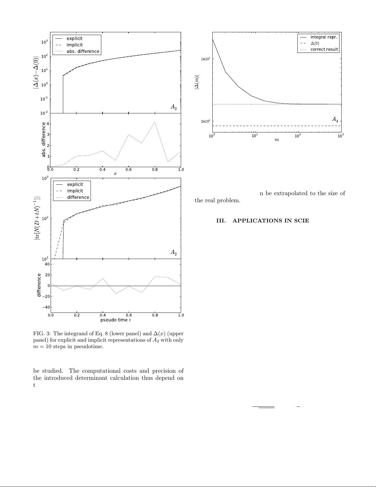
Sto c hastic determination of matrix determinan ts Sebastian Dorn ∗ and T orsten A. Enßlin Max-Planck-Institut f¨ ur Astr ophysik, Karl-Schwarzschild-Str. 1, D-85748 Gar ching, Germany Ludwigs-Maximilians-Universit¨ at M¨ unchen, Geschwister-Schol l-Platz 1, D-80539 M¨ unchen, Germany (Dated: July 8, 2015) Matrix determinants pla y an imp ortan t role in data analysis, in particular when Gaussian pro- cesses are inv olved. Due to curren tly explo ding data volumes, linear op erations – matrices – acting on the data are often not accessible directly but are only represented indirectly in form of a com- puter routine. Suc h a routine implements the transformation a data vector undergo es under matrix m ultiplication. While efficient probing routines to estimate a matrix’s diagonal or trace, based solely on suc h computationally affordable matrix-vector m ultiplications, are w ell known and fre- quen tly used in signal inference, there is no stochastic estimate for its determinant. W e introduce a probing metho d for the logarithm of a determinant of a linear operator. Our metho d rests upon a reformulation of the log-determinant by an integral representation and the transformation of the in volv ed terms in to stochastic expressions. This sto c hastic determinan t determination enables large- size applications in Bay esian inference, in particular evidence calculations, model comparison, and p osterior determination. Keyw ords: Determinants – Stochastic Estimation – Op erator Probing – Big Data – Signal Inference I. MOTIV A TION Curren t and future physical observ ations generate h uge data streams to b e analyzed. Particle ph ysics, biophysics, astronom y , and cosmology are represen tatives of curren t scien tific fields of in terest that are undergoing a revo- lution driv en b y increasing data volume. T ypical large data sets in cosmology are, for instance, observ ations of the cosmic microw a ve background [1, 2] as w ell as of the large-scale structure [3 – 5] as they are often wide- or all- sky observ ations carried out by telescop es with remark- able resolution. In order to extract information ab out the univ erse or ph ysics in general, Ba y esian inference meth- o ds b ecomes more and more frequen tly used as their large computational demands b ecome more feasible thanks to tec hnology developmen ts. The signal of in terest to b e extracted from data could b e almost everything, ranging from just a single parameter (e.g., the level of local non- Gaussianit y of the cosmic micro wa v e background [6, 7]) to a full four-dimensional reconstruction of the structure gro wth in the universe [8, 9]. Suc h ambitious Ba yesian analyses often in vok e linear transformations of the data or of estimated signal vectors. The size of the in volv ed data and signal spaces of- ten bans the explicit represen tation of matrices acting on these spaces by their individual matrix elements. A prominen t example appearing in many analyses is, for in- stance, the cov ariance matrix of a multiv ariate Gaussian distribution of a vector v alued quantit y , which describ es the t w o-p oin t correlation structure of the said quan tity . Due to their large dimensions suc h matrices are often only represen table b y a computer routine, which imple- men ts the application of the matrix to a v ector with- ∗ sdorn@mpa-garching.mpg.de out storing or even calculating the individual matrix el- emen ts. Such routines often inv ok e fast F ourier transfor- mations and other efficien t op erations, whic h in combi- nation render nonsparse matrices into easily computable basis systems. W e refer to suc h a matrix as an implicit matrix . F or instance, calculating the mo del evidence of- ten requires calculating determinants of such matrices. This work pro vides an efficient wa y to numerically calcu- late determinan ts giv en only b y an implicit matrix rep- resen tation. The remainder of this work is organized as follows: In Sec. I I we introduce the formalism of the sto chastic esti- mation of an implicit matrix and present tw o numerical examples. Section II I provides a persp ective of p ossi- ble applications in science. Results are summarized in Sec. IV. I I. PR OBING THE LOG-DETERMINANT OF AN IMPLICIT MA TRIX A. F ormalism Let A = ( a ij ) ∈ C n × n b e an implicitly defined, complex-v alued, square matrix of order n . Implicitly means that the particular entries of the matrix are not accessible, for instance, if dealing with large data sets, where an explicit storage of A might exceed the memory of the computer. How ev er, the action of the matrix as a linear op erator is assumed to be kno wn and giv en by a computer routine implemen ting the mapping x 7→ Ax . Motiv ated by applications in science and statistics (Secs. I and I II), in particular b y signal reconstruction tec hniques and mo del comparison in astronomy and cos- mology , where the determinant of a cov ariance matrix is required (Sec. I II), we constrain the v ariet y of differ- en t types of matrices b y requesting that the matrix A of 2 in terest is either we ak diagonal dominant or Hermitian p ositive definite . The term we ak diagonal dominant is defined by | a ii | ≥ X i 6 = j | a ij | ∀ i, (1) while Hermitian p ositive definite means A † = A and x † Ax > 0 ∀ x ∈ C n \{ 0 } (2) with † denoting the adjoint. The diagonal and the trace of an implicit matrix can b e obtained by exploiting common probing routines [10– 13]. A stochastic estimate of the diagonal of the linear op erator A is given by diag( A ) = h ξ ? Aξ i { ξ } ≈ 1 M M X i =1 ξ i ? Aξ i , (3) where ? denotes a comp onen twise pro duct, M = |{ ξ }| the sample size, and h·i { ξ } the arithmetic mean o ver ξ with M → ∞ . The probing v ectors ξ ∈ C n are random v ariables, whose comp onents x ( x 0 ) fulfill the condition h ξ x ξ x 0 i { ξ } = δ xx 0 . Analogously to the diagonal of an op erator its trace can be prob ed by , e.g., tr( A ) =  ξ † Aξ  { ξ } . (4) Recen tly , there hav e b een inv estigations to improv e these straigh tforward probing metho ds by exploiting Ba yesian inference [10]. This has be en achiev ed by re- form ulating the pro cess of sto c hastic probing of an op er- ator’s diagonal (trace) as a signal inference problem. As a result, it requires few er prob es than the purely sto chastic metho ds and th us can decrease the computational costs. With the phrase op er ator pr obing , b e it trace or diagonal probing, w e subsequently refer to the entiret y of probing metho ds in general. The linear op erator A can b e split into a diagonal ma- trix D ∈ C n × n and a matrix N ∈ C n × n , which contains the off-diagonal part of A , i.e., A = D + N . (5) W e are now in terested in the v alue of its determinan t or of its log-determinant, ∆ ≡ ln[det( A )]. In case A is mainly dominated b y its diagonal (i.e. N D − 1  1 spectrally), a T a ylor expansion of the log-determinant might b e a reasonable approximation, ∆ = ln[det( D + N )] = ln[det( D )] + tr  N D − 1  + O  tr h  N D − 1  2 i , (6) whic h is sometimes feasible dealing with implicit op er- ators, e.g., see Refs. [7, 14] for recent applications in cosmic micro w av e background physics. This approxima- tion, ho w ev er, breaks do wn when the relation N D − 1  1 (sp ectrally) is violated. In order to circumv en t this prob- lem we introduce the quantit y ∆( t ) ≡ ln[det( D + tN )] (7) with the pseudotime parameter t ∈ [0 , 1]. F or a suf- ficien tly small t the approximation of Eq. (6) b ecomes v alid. This prop ert y can be used together with a few mathematical manipulations (for details see App endix A) to obtain the formula ∆ = Z 1 0 dt tr h N ( D + tN ) − 1 i + ∆(0) = Z 1 0 dt D ξ † N ( D + tN ) − 1 ξ E { ξ } + ∆(0) (8) that represen ts a sto c hastic estimate of the log- determinan t of A using operator probing. In particular, the following steps are required to ev aluate Eq. (8): 1. Diagonal (operator-) probing to split A into A = diag ( A ) | {z } ≡ D + A − diag ( A ) | {z } ≡ N , 2. an approach to inv ert D + tN in Eq. (8), e.g., the conjugate gradient method [15], 3. trace (operator-) probing to ev aluate the integrand, 4. a numerical integration metho d, e.g., applying Simpson’s rule. It might immediately strike the eye of the reader that one recaptures the simple first-order T aylor-expanded v ersion of the log-determinant, Eq. (6), when dropping the pseudotime dep endency of the integrand in Eq. (8) b y requesting t = 0. This means that in case of deal- ing with diagonal dominant op erators the v alue of the correct log-determinan t might b e received by a coarse n umerical in tegration since the integrand close to t = 0 already yields the main correction, which might decrease the computational costs, see Sec. I I B. Equation (8) further represents the main result of this pap er and can b e regarded as a special case of calculat- ing partition functions (see Sec. I I I and Refs. [16, 17]). Although the first line of it, the integral representation of the log-determinant, was also, indep endently of our work, found by mathematicians 10 years ago [18], it is (to our kno wledge) not known in the communit y of ph ysics or sig- nal inference. The connection to sto c hastic estimators, ho wev er, is a no vel w ay to ev aluate the log-determinant of implicitly defined matrices that enables previously im- p ossible calculations, see Sec. II I. B. Numerical example W e address here a simple and also exactly solv able nu- merical example referring to (Bay esian) signal inference 3 problems or, in general, statistical problems in physics (see Secs. I II A and I I I B), where the log-determinant of a cov ariance matrix A is of in terest. If we assume statistical isotropy and homogeneity of a ph ysical field, its cov ariance matrix can b e parametrized b y a so-called p o w er sp ectrum. This is often a reasonable assumption 1 , e.g., in astronom y and physical cosmology , when apply- ing the cosmological principle. In this case the co v ariance matrix b ecomes diagonal in F ourier space, A kk 0 = c k δ kk 0 , (9) with resp ective F ourier mo des k , k 0 and p ow er sp ectrum c k . It is straigh tforward to sho w that the p osition space represen tation of A kk 0 , giv en b y A xx 0 = F † xk A kk 0 F k 0 x 0 with F ourier transformation F , is nondiagonal if and only if c k 6 = const ∀ k . In order to apply the sto chastic esti- mator of the log-determinant we use tw o sp ecial forms of the p ow er sp ectrum, given by c k = 1 (1 + k ) α (10) with α set to 2 or 4. A v alue of α = 2 describ es a mostly diagonal dominant matrix, whereas α = 4 exhibits a significant nondiagonal structure in p osition space. T o b e precise, in the follo wing we use a regular, t wo-dimensional, real-v alued grid (o ver T 2 ) of n = 20 × 20 pixels to represent our p osition space, resulting in a ma- trix A consisting of n × n = 1 . 6 × 10 5 real num b ers. See Fig. 1 for an illustration thereof. F or b oth matrices, which we refer to as A 2 and A 4 , w e apply Eq. (8) given an explicit and implicit numerical implemen tation. F or the explicit v arian t there also exist w ell-understo o d, precise numerical methods 2 to calculate the determinant. Therefore, the n umerical results of such a metho d can be regarded as our gold standard and hence serv e as a reference for the probing results. Henceforth w e will refer to it using the subscript “correct”. Both v arian ts, the explicit and implicit implementation, are realized using the to ols of NIFTy [19]. After the separation of A 2 and A 4 in to diagonal and off-diagonal parts by applying diagonal probing w e calcu- late the in tegrands of Eq. (8) for the m -part-discretized in terv al of t ∈ [0 , 1] by using the conjugate gradient metho d as w ell as trace probing and perform the numeri- cal integration afterwards by using Simpson’s rule. The op erator probing as well as the conjugate gradient metho d hav e also b een realized using NIFTy . F urther- more we introduce the quantities ∆( x ) ≡ Z x 0 dt tr h N ( D + tN ) − 1 i + ∆(0) , x ∈ [0 , 1] (11) 1 Referring to Bay esian evidence calculations such a matrix might be the prior or p osterior cov ariance, see Sec. II I for details. 2 See, for instance, the metho d described at http: //docs.scipy.org/doc/numpy/reference/generated/numpy. linalg.slogdet.html , which is based on LU-factorization. A 2 0.2 15.0 A 4 0.2 4.7 FIG. 1: Illustration of the matrices A 2 (top) and A 4 (b ottom) in p osition space with linear color bars. to study the conv ergence to the final v alue and ∆( m ) to in vestigate the dep endency on the discretization of the in tegration in terv al, see Figs. 2, 3, and 4. W e used a rather low sample size of M = 8 for trace and diagonal probing [see Eqs. (4) and (3)] to demon- strate the applicabilit y of the metho d to large data sets. The discretization of the pseudotime in terv al in to m parts w as c hosen to b e m = 10 3 for A 4 and only m = 10 for A 2 , see in particular Fig. 4, which illustrates the dep endence of the probing result on m . 4 T ABLE I: Results of the numerical determinant calculations with and without probing. The absolute errors of the probing metho d are defined b y  1 = | ∆ explicit (1) − ∆ implicit (1) | and  2 = | ∆ correct − ∆ implicit (1) | . Differences b et ween  1 and  2 arise from the discretized, numerical in tegration. A 2 A 4 ∆(0) -1308.05 -1771.57 ∆ correct -1566.99 -3107.28 ∆ explicit (1) -1566.81 -3107.29 ∆ implicit (1) -1565.33 -3108.41 m 10 1000 M 8 8  1 1.48 1.12  2 1.66 1.13 C. Discussion The exact numerical v alues of the determinant calcu- lation using explicit and implicit representations of A 4 and A 2 can b e found in T able I. The results of the prob- ing method (implicit) compared to the correct and the explicit metho d, where Eq. (8) can b e ev aluated without using a conjugate gradient or probing techniques, are accurate for b oth matrices. It is remark able that despite using a relatively small sample size of M = 8 the abso- lute errors remain relatively small. The reason for this is that the pseudotime integration ov er all prob ed in te- grands a v erages the probing error. This is of particular imp ortance when applying the log-determinant probing to large data sets, where a large sampling size should b e a voided to sav e computational time. These errors can b e decreased further, of course, b y an increase of the sam- pling size and a refinement of the numerical integration. The results of the trace (integrand) probing and the determinan t’s conv ergence b ehavior as well as their re- sp ectiv e errors with respect to the explicit represen tation can b e found in Figs. 2 and 3. Note that the scaling of the ordinate is logarithmic. F or both matrices, but esp ecially for A 4 , the largest contribution to the integral of Eq. (8) comes from late t -v alues. Therefore, if dealing with big data sets, one could divide the integration in terv al not in to m equal parts but by starting with a rather coarse discretization for small t -v alues and subsequently refin- ing it for larger v alues, e.g., by substituting dt by d ln( t 0 ) and thereby saving computational costs. This, how ev er, migh t depend on the particular shape of the matrix and has to b e studied case by case. The dependency of the numerical v alue of the deter- minan t of A 4 on the discretization (in m equal parts) of the integration interv al can b e found in Fig. 4 and sho ws that ev en a small v alue of m adds significant cor- rections to the result. The result for m ∝ O (10) is, for instance, b etter than just using the determinan t of the diagonal, ∆(0). This migh t b e used in practice to in- v estigate cheaply whether the nondiagonal structure of a matrix influences the determinant significantly . x 1 0 - 2 1 0 - 1 1 0 0 1 0 1 1 0 2 1 0 3 1 0 4 | ∆ ( x ) − ∆ ( 0 ) | A 4 0.0 0.2 0.4 0.6 0.8 1.0 x 0.0 0.5 1.0 1.5 abs. difference explicit implicit (below explicit) abs. difference p s e u d o t i m e t 1 0 1 1 0 2 1 0 3 1 0 4 | t r [ N ( D + t N ) − 1 ] | A 4 0.0 0.2 0.4 0.6 0.8 1.0 p s e u d o t i m e t 400 200 0 200 400 difference explicit implicit difference FIG. 2: The in tegrand of Eq. 8 (lo w er panel) and ∆( x ) (upper panel) for explicit and implicit represen tations of A 4 . A h uge adv an tage of the probing method discussed here is the possibility to parallelize the n umerical calcula- tion almost completely . T o b e precise, the diagonal prob- ing b eforehand, the pseudotime integral, as w ell as every single trace probing can b e parallelized fully . The only op eration that cannot b e parallelized is the conjugate gradient metho d as it is a p otential minimizer, using at least the previous step to calculate the next one. The determination of a suitable choice of the in volv ed parameters m and M as well as the precision parameters for the used conjugate gradient approach and n umer- ical integration metho d dep end highly on the matrix to 5 x 1 0 - 2 1 0 - 1 1 0 0 1 0 1 1 0 2 1 0 3 | ∆ ( x ) − ∆ ( 0 ) | A 2 0.0 0.2 0.4 0.6 0.8 1.0 x 0 1 2 3 4 abs. difference explicit implicit abs. difference p s e u d o t i m e t 1 0 1 1 0 2 1 0 3 | t r [ N ( D + t N ) − 1 ] | A 2 0.0 0.2 0.4 0.6 0.8 1.0 p s e u d o t i m e t 40 20 0 20 40 difference explicit implicit difference FIG. 3: The in tegrand of Eq. 8 (lo w er panel) and ∆( x ) (upper panel) for explicit and implicit representations of A 2 with only m = 10 steps in pseudotime. b e studied. The computational costs and precision of the introduced determinant calculation thus dep end on the combination of the chosen metho ds for diagonal and trace probing, n umerical integration, the metho d to nu- merically in vert the matrix D + tN , and the matrix A itself. Since it is therefore not possible to mak e general statemen ts we consciously av oid here suc h a discussion of computational costs and precision with resp ect to m and M . A more pragmatic wa y to estimate these param- eters would b e to downscale the problem of interest un til the matrix of interest fits into the memory of the com- 1 0 0 1 0 1 1 0 2 1 0 3 m 2 x 1 0 3 1 x 1 0 4 | ∆ ( m ) | A 4 integral repr. ∆ ( 0 ) correct result FIG. 4: Dep endency of the determinan t’s result on the dis- cretization of the integration interv al into m parts, using A 4 . puter and to subsequently p erform mock tests to obtain a suitable choice for the parameters discussed ab ov e. Af- terw ards these v alues can b e extrap olated to the size of the real problem. I II. APPLICA TIONS IN SCIENCE Within this section we presen t a selection of p ossible applications in science. Although there are a v ast num- b er of research fields and topics which might b enefit from the sto c hastic estimation of a log-determinan t we focus henceforth on a selection of usages in Bay esian signal inference, in particular in ph ysics and only presen t sim- ple examples. Exact, more complicated examples can b e found in the cited works within this section. A. Evidence calculations & mo del selection The Bay esian evidence P ( d ) is a measure for the qual- it y of the mo del and hence for all assumed mo del param- eters for the data d [20]. T o keep it short and simple w e assume a mo del that describes a linear measuremen t of a Gaussian signal s with additive, signal-indep endent, Gaussian noise n , i.e., d = R s + n, (12) where R represents a linear op erator. A Gaussian distri- bution of a v ariable x is defined by P ( x ) = G ( x, X ) ≡ 1 p | 2 π X | exp  − 1 2 x † X − 1 x  (13) with related co v ariance matrix X and mean h x i P ( x ) ≡ Z D x x P ( x ) . (14) 6 R D [ · ] denotes a phase space in tegral and | · | the deter- minan t. Under these circumstances the evidence can be calculated as P ( d ) = Z D s Z D n P ( d, s, n ) = Z D s Z D n δ ( d − Rs − n ) P ( n | s ) P ( s ) = s | 2 π C s | d | | 2 π C s || 2 π C n | exp  − 1 2  d † C − 1 n d − j † C s | d j   , (15) with j = R † C − 1 n d, C − 1 s | d = R † C − 1 n R + C − 1 s , (16) and the signal and noise co v ariances C s and C n , respec- tiv ely . Therefore, to calculate the Bay esian model evi- dence, one often 3 has to calculate determinants of co v ari- ance matrices. This might b e done by probing [Eq. (8)] if dealing with implicit matrices [last line of Eq. (15)] instead of p erforming the multidimensional integral [sec- ond last line in Eq. (15)] numerically . The latter has b een done, for instance, in the field of inflationary cos- mology [21, 22] by the method of nested sampling [23, 24]. This is esp ecially of imp ortance in the field of mo del selection or comparison [20], where from an observ ation – the data – one w an ts to infer which theory repro duces the observ ation b est. Switc hing from one model to another means, for instance 4 , to exc hange R in Eq. (15), which directly affects the determinant con taining C s | d . Thus, the calculation of the determinant is mandatory here. B. P osterior distribution including marginalizations In the field of signal inference one is typically in ter- ested in reconstructing a set of i parameters p i with un- certain ty from some observ ation, the data d . This in- formation is delivered by the p osterior, given by 5 [25] P ( p i | d ) ∝ P ( d | p i ) P ( p i ). Often, how ev er, this inference problem is degenerate, caused by a so-called nuisance pa- rameter. F or example, consider the calibration of an in- strumen t is of interest and not the signal. In this case the signal s represents the nuisance parameter. The common 3 By the w ord “often” we refer to cases, in whic h at least one marginalization [see Eq. (17)] can be p erformed analytically (ap- proximated with high precision) to obtain a mo del-dependent determinant. 4 W e fo cus here on R for simplicit y only . One could also, addi- tionally , exchange the prior cov ariances C n and C s , the assumed prior statistics, the parametrization of the data, and so on. 5 Note that in this case the evidence is just a scalar which normal- izes the p osterior, therefore we merely state prop ortionalities. pro cedure to circum ven t this problem is to marginalize o ver these parameters, P ( p i | d ) ∝ Z D s Z D n P ( d, s, n | p i ) P ( p i ) . (17) T o con tinue with the simple example of Sec. I II A we assume again Gaussian distributions for s and n and a linear measurement but with explicit dep endency on p i , i.e., d = ( Rs )[ p i ] + n . If we further follo w the example of calibration, the parameter p i migh t b e a calibration co efficien t, thus affecting only R . This yields ( Rs )[ p i ] = R [ p i ] s and therefore P ( p i | d ) ∝  Z D s G  d − R [ p i ] s, C n  G ( s, C s )  P ( p i ) . (18) This in tegration can be p erformed analytically , produc- ing an in general non-Gaussian probabilit y distribution with p i -dep enden t normalization (and exp onent) similar to Eq. (15), P ( p i | d ) ∝ q   2 π C s | d [ p i ]   P ( p i ) × exp  1 2 j † [ p i ] C s | d [ p i ] j [ p i ]  (19) with C s | d [ p i ] and j [ p i ] now con taining R [ p i ] instead of R . In case the co v ariance matrices or R [ p i ] are only giv en b y a computer routine (implicit representation of a matrix) one could use Eq. (8) to prob e the determinan t. A v ariety of scien tific fields are affected b y this prob- lem. F or example, the extraction of the level of non- Gaussianit y of the cosmic microw a ve background [7, 14] in cosmology , the problem of self-calibration [26 – 28] in general, or lensing in astronomy [29]. C. Realistic astronomical example In order to study a more realistic example w e consider a measuremen t device with spatially constant but un- kno wn calibration amplitude, parametrized by 1 + γ ∈ R , scanning a specific patc h of the sky . The measured and assumed to b e Gaussian sky signal s is affected by the instrumen t via a conv olution C with a Gaussian kernel of standard deviation σ = 0 . 05. Additionally , the observ a- tion migh t b e disturb ed b y fore- and bac kgrounds. F or this reason w e include an observ ational mask M o , which cuts out 20% of the sky . The noise n is still assumed to b e Gaussian and uncorrelated with the signal. Hence, the measurement equation is given by d = R [ γ ] s + n = (1 + γ ) M o C s + n. (20) T o calibrate the measurement device the calibration pos- terior P ( γ | d ) has to b e determined. The resulting cal- ibration mean h γ i P ( γ | d ) can b e regarded as an external calibration if the a priori kno wledge on the signal is suf- ficien tly strong. Otherwise one could infer the signal and 7 calibration amplitude γ simultaneously from data using iterativ e approac hes [27]. Using Eq. (19) as well as a flat prior on γ w e obtain ln P ( γ | d ) = − 1 2 ln    C − 1 s | d [ γ ]    + 1 2 j † [ γ ] C s | d [ γ ] j [ γ ] + const ., (21) whic h exhibits in particular the γ -dep enden t determinant    C − 1 s | d [ γ ]    =   (1 + γ ) C † M † o C − 1 n M o C (1 + γ ) + C − 1 s   . (22) F or the numerical ev aluation of Eq. (21) we use the settings of Sec. I I B with C s ( k , k 0 ) = (1 + k ) − 3 δ kk 0 , a calibration amplitude parameter of γ = 2, and a noise co v ariance of ( C n ) x,x 0 = 10 − 1 δ xx 0 to generate a data re- alization. The pseudotime interv al has b een discretized in to 10 2 parts. The numerically determined calibration p osterior for a given data realization can b e found in Fig. 5, which demonstrates again the efficiency of the sto c hastic metho d using only eight prob es for a single trace probing op eration. The figure also illustrates the impact of the determinant on the log-p osterior, which w ould not p eak in the shown interv al without it. 0 2 4 6 8 10 γ 0 100 200 300 400 500 l n [ P ( γ | d ) ] + c o n s t . explicit implicit n e g l e c t i n g ∆ + c o n s t . correct value FIG. 5: Logarithmic posterior of the calibration amplitude parameter γ using implicit and explicit representations of the in volv ed op erators, see Eq. (21) and Eq. (22) for details. The abbreviation ∆ denotes the logarithm of the term given by Eq. (22). IV. SUMMAR Y Motiv ated b y the problem of finding a wa y to efficien tly determine the determinant of an implicitly defined ma- trix or op erator, we deriv ed a formula, Eq. (8), repre- sen ting a stochastic estimate of its log-determinan t. This has b een achiev ed by reform ulating the log-determinant as an in tegral representation and transforming the in- v olved terms into stochastic expressions, whic h includes a numerical in tegration and a trace probing. Numerical examples ha v e sho wn that the discretization of the inte- gration in terv al may b e v ery coarse in case the prob ed op erator is sufficiently diagonal. In case it exhibits a sig- nifican t nondiagonal structure one has to fine-grain the discretization of this interv al. The num ber of probes nec- essary for the trace probing, ho wev er, remains very lo w in the studied examples. These facts com bined with the almost complete parallelizability of this approach might k eep the computational costs within reasonable limits in man y situations. This metho d clearly has more general applications but migh t in particular b e useful for Bay esian signal inference and mo del comparison when dealing with large data sets as often giv en, for instance, in astronomy and cosmology . T o be precise, it might b e beneficial in all fields where the n umerical calculation of a determinan t of an operator is mandatory . Ac knowledgmen ts W e gratefully ackno wledge Maksim Greiner for dis- cussions and David Butler for useful comments on the man uscript. All calculations w ere realized using NIFTy [19] to b e found at http://www.mpa- garching.mpg.de/ ift/nifty . App endix A: In tegral representation of the log-determinan t of a matrix Here Eq. (8) is derived. F ollowing Sec. I I the log- determinan t ∆ of an op erator A can b e parametrized b y ∆ = ln[det( D + N )] with D b eing the diagonal and N the off-diagonal part of A . Since ∆ can b e T aylor- expanded for small N (sp ectrally compared to D ) only , w e employ a metho d from the field of renormalization theory [28, 30]. Accordingly , we in tro duce an expansion parameter δ t  1 to suppress the influence of N . In par- ticular, we replace ∆ by ln[det( D + δ tN )] for a moment. F or sufficien tly small v alues of δ t , in the following inter- preted as tiny pseudotime steps, we can approximate ∆ b y Eq. (6). Theoretically , a single pseudotime step could b e infinitesimal small, enabling the formal definition of the deriv ativ e d ∆( t ) dt ≡ lim δ t → 0 ln[det( D + ( t + δ t ) N )] − ln[det( D + tN )] δ t = lim δ t → 0 1 δ t ln  det  1 + δ tN [ D + tN ] − 1  = lim δ t → 0 1 δ t tr  ln  1 + δ tN [ D + tN ] − 1  = tr  N [ D + tN ] − 1  , (A1) with the definition ∆( t ) ≡ ln[det( D + tN )] . (A2) 8 In tegrating the pseudotime deriv ativ e of ∆( t ) yields the in tegral represen tation of the log-determinant, ∆ = Z 1 0 dt tr h N ( D + tN ) − 1 i + ∆(0) . (A3) This integral represen tation has also b een found by Ref. [18], where its v alidit y has b een prov en for weak diagonal dominan t and Hermitian p ositive definite ma- trices. In particular one has to ensure the existence of the inv erse matrix of the integrand of Eq. (A3). Finally , w e replace the trace b y sto c hastic trace prob- ing and p erform the pseudotime integral by an numeric in tegration method. This yields ∆ = Z 1 0 dt D ξ † N ( D + tN ) − 1 ξ E { ξ } + ∆(0) . (A4) [1] C. L. Bennett, D. Larson, J. L. W eiland, N. Jarosik, G. Hinshaw, N. Odegard, K. M. Smith, R. S. Hill, B. Gold, M. Halp ern, et al., Astrophys. J. Suppl. Ser. 208 , 20 (2013), 1212.5225. [2] Planck Collab oration, P . A. R. Ade, N. Aghanim, C. Armitage-Caplan, M. Arnaud, M. Ashdown, F. A trio- Barandela, J. Aumon t, C. Baccigalupi, A. J. Banday , et al., Astronomy and Astrophysics 571 , A16 (2014), 1303.5076. [3] D. G. Y ork, J. Adelman, J. E. Anderson, Jr., S. F. An- derson, J. Annis, N. A. Bahcall, J. A. Bakken, R. Bark- houser, S. Bastian, E. Berman, et al., The Astronomical Journal 120 , 1579 (2000), astro-ph/0006396. [4] D. N. Spergel, R. Bean, O. Dor´ e, M. R. Nolta, C. L. Ben- nett, J. Dunkley , G. Hinsha w, N. Jarosik, E. Komatsu, L. P age, et al., Astroph ys. J. Suppl. Ser. 170 , 377 (2007), astro-ph/0603449. [5] G. J. Hill, K. Gebhardt, E. Komatsu, N. Drory, P . J. MacQueen, J. Adams, G. A. Blanc, R. Ko ehler, M. Rafal, M. M. Roth, et al., Astronomical Society of the P acific Conference Series 399 , 115 (2008), 0806.0183. [6] E. Komatsu, D. N. Sp ergel, and B. D. W andelt, Astro- ph ys. J. 634 , 14 (2005), arXiv:astro-ph/0305189. [7] S. Dorn, N. Opp ermann, R. Khatri, M. Selig, and T. A. Enßlin, Phys. Rev. D 88 , 103516 (2013), 1307.3884. [8] F. S. Kitaura and T. A. Enßlin, MNRAS 389 , 497 (2008), 0705.0429. [9] J. Jasche and B. D. W andelt, MNRAS 432 , 894 (2013), 1203.3639. [10] M. Selig, N. Opp ermann, and T. A. Enßlin, Phys. Rev. E 85 , 021134 (2012), 1108.0600. [11] E. Aune, D. Simpson, and J. Eidsvik, Statistics and Com- puting 24 , 247 (2014), ISSN 0960-3174. [12] M. Hutc hinson, Comm unications in Statistics - Simula- tion and Computation 18 , 1059 (1989). [13] C. Bek as, E. Kokiop oulou, and Y. Saad, Applied Numer- ical Mathematics 57 , 1214 (2007). [14] S. Dorn, E. Ramirez, K. E. Kunze, S. Hofmann, and T. A. Enßlin, Journal of Cosmology and Astro-P article Ph ysics 6 , 048 (2014), 1403.5067. [15] M. R. Hestenes and E. Stiefel, Journal of Research of the National Bureau of Standards 49 , 409 (1952). [16] M.-D. W u and W. Fitzgerald, Bayesian Multimo dal Evi- denc e Computation by A dapti T empering MCMC , vol. 79 of F undamental The ories of Physics (Springer Nether- lands, 1996). [17] D. C. M. Dickson, M. R. Hardy , and H. R. W aters, Physics and Prob ability - Essays in Honor of Edwin T. Jaynes (Cam bridge Universit y Press, Cambridge, 2004), 1st ed., ISBN 978-0-521-61710-9. [18] J. Du and J. Ji, Dynamical Systems 2005 , 225 (2005). [19] M. Selig, M. R. Bell, H. Junklewitz, N. Opp ermann, M. Reineck e, M. Greiner, C. P acha joa, and T. A. Enßlin, Astronomy and Astrophysics 554 , A26 (2013), 1301.4499. [20] E. Jaynes and G. Bretthorst, Pr ob ability The ory: The L o gic of Scienc e, Chapter 12.4 (Cambridge Universit y Press, 2003), ISBN 9781139435161. [21] Planck Collab oration, P . A. R. Ade, N. Aghanim, C. Armitage-Caplan, M. Arnaud, M. Ashdown, F. A trio- Barandela, J. Aumon t, C. Baccigalupi, A. J. Banday , et al., Astronomy and Astrophysics 571 , A22 (2014), 1303.5082. [22] J. Martin, C. Ringev al, R. T rotta, and V. V ennin, Journal of Cosmology and Astro-P article Ph ysics 3 , 039 (2014), 1312.3529. [23] J. Skilling, AIP Conference Proceedings 735 , 395 (2004). [24] F. F eroz, M. P . Hobson, and M. Bridges, MNRAS 398 , 1601 (2009), 0809.3437. [25] T. Bay es, Phil. T rans. of the Roy . So c. 53 , 370 (1763). [26] S. L. Bridle, R. Crittenden, A. Melchiorri, M. P . Hob- son, R. Kneissl, and A. N. Lasenb y, MNRAS 335 , 1193 (2002), astro-ph/0112114. [27] T. A. Enßlin, H. Junklewitz, L. Winderling, M. Greiner, and M. Selig, Ph ys. Rev. E 90 , 043301 (2014), 1312.1349. [28] S. Dorn, T. A. Enßlin, M. Greiner, M. Selig, and V. Bo ehm, Phys. Rev. E 91 , 013311 (2015), 1410.6289. [29] C. M. Hirata and U. Seljak, Phys. Rev. D 67 , 043001 (2003), astro-ph/0209489. [30] T. A. Enßlin and M. F rommert, Ph ys. Rev. D 83 , 105014 (2011), 1002.2928.