Parallel matrix factorization for low-rank tensor completion
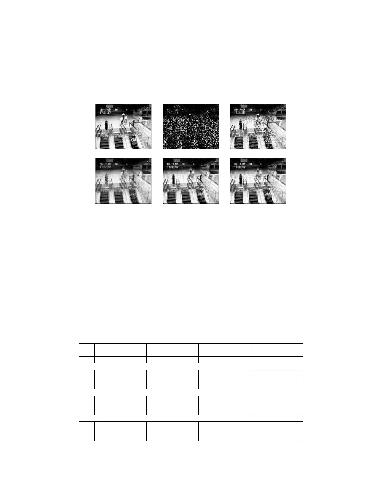
Higher-order low-rank tensors naturally arise in many applications including hyperspectral data recovery, video inpainting, seismic data recon- struction, and so on. We propose a new model to recover a low-rank tensor by simultaneously performing low…
Authors: Yangyang Xu, Ruru Hao, Wotao Yin
Inverse Problems and Imaging doi:10.3934/xx.xx.xx.xx Volume X, No. 0X, 200X, X–XX P ARALLEL MA TRIX F A CTORIZA TION F OR LO W-RANK TENSOR COMPLETION Y angy ang Xu Department of Computational and Applied Mathematics, Rice Universit y Houston, TX 77005, USA R uru Ha o School of Mathematical Sciences, Dalian Universit y of T echnology , Dalian, China. W ot a o Yin Department of Mathematics, Universit y of California, Los Angeles, CA 90095, USA Zhixun Su School of Mathematical Sciences, Dalian Universit y of T echnology , Dalian, China. Abstract. Higher-order low-rank tensors naturally arise in man y applications including hypersp ectral data recov ery , video inpainting, seismic data recon- struction, and so on. W e propose a new mo del to recov er a lo w-rank tensor by simultaneously p erforming low-rank matrix factorizations to the all-mode ma- tricizations of the underlying tensor. An alternating minimization algorithm is applied to solv e the mo del, along with t wo adaptiv e rank-adjusting strategies when the exact rank is not kno wn. Phase transition plots rev eal that our algorithm can recov er a variet y of synthetic lo w-rank tensors from significantly few er samples than the compared methods, which include a matrix completion method applied to tensor reco very and tw o state-of-the-art tensor completion metho ds. F urther tests on real- world data show similar adv antages. Although our model is non-conv ex, our algorithm p erforms consistently throughout the tests and giv es b etter results than the compared methods, some of which are based on conv ex models. In addition, subsequence conv ergence of our algorithm can b e established in the sense that an y limit point of the iterates satisfies the KKT condtions. 1. In tro duction. T ensor is a generalization of ve ctor and matrix . A vector is a first-order (also called one-wa y or one-mo de) tensor, and a matrix is a second-order tensor. Higher-order tensor arises in many applications suc h as 3D image reconstruc- tion [ 22 ], video inpainting [ 19 ], h yp ersp ectral data recov ery [ 14 , 28 ], higher-order w eb link analysis [ 10 ], p ersonalized web searc h [ 23 ], and seismic data reconstruction [ 11 ]. In this pap er, we fo cus on the recov ery of higher-order tensors that are (ex- actly or appro ximately) low-rank and hav e missing entries. W e dub the problem as low-r ank tensor c ompletion (LR TC). The introduced mo del and algorithm can b e extended in a rather straightforw ard wa y to recov ering lo w-rank tensors from their linear measuremen ts. LR TC can b e regarded as an extension of low-rank matrix completion [ 1 ]. T o reco ver a low-rank tensor from its partially observed en tries, one can unfold it into a 2010 Mathematics Subje ct Classific ation. Primary: 94A08, 94A12; Secondary: 90C90. Key words and phr ases. higher-order tensor, lo w-rank matrix completion, lo w-rank tensor com- pletion, alternating least squares, non-con vex optimization. 1 c 200X American Institute of Ma thema tical Sciences 2 Y. Xu, R. Hao, W. Yin and Z. Su matrix and apply a low-rank matrix completion algorithm such as FPCA [ 17 ], APGL [ 24 ], LMaFit [ 27 ], the alternating direction method [ 2 , 31 ], the ` q minimization metho d [ 13 ], and so on. Ho wev er, this kind of metho d utilizes only one mo de lo w-rankness of the underlying tensor. W e are motiv ated and convinced b y the results [ 16 ] that utilizing all mo de low-ranknesses of the tensor gives muc h b etter p erformance. Existing methods for LR TC in [ 16 , 3 ] employ matrix nuclear-norm minimization and use the singular v alue decomp osition (SVD) in their algorithms, which b ecome v ery slow or even not applicable for large-scale problems. T o tackle this difficult y , w e apply low-r ank matrix factorization to each mode unfolding of the tensor in order to enforce low-rankness and up date the matrix factors alternativ ely , whic h is computationally m uch cheaper than SVD. Our approac h is non-conv ex, and the sizes of the matrix factors must be sp ecified in the algorithm. Non-conv exity mak es it difficult for us to predict the p erformance of our approac h in a theoretical wa y , and in general, the p erformance can v ary to the c hoices of algorithm and starting p oint. W e found cyclic up dates of the unknown v ariables in the mo del to p erform well enough. The sizes of the matrix factors dictate the rank of the recov ered tensor. If they are fixed to v alues significantly different from the true rank, the recov ery can ov erfit or underfit. On the other hand, during the run time of our algorithms, there are simple wa ys to adaptiv ely adjust the factor sizes. In short, the all-mode matricizations, cyclic block minimization, and adaptiv e adjustmen t are the building blocks of our approach. Before in tro ducing our mo del and algorithm, we review some notation and tensor op erations. 1.1. Notation. F ollowing [ 9 ], we use b old lo w er-case letters x , y , . . . for v ectors, b old upp er-case letters X , Y , . . . for m atrices, and b old caligraphic letters X , Y , . . . for tensors. The ( i 1 , . . . , i N )-th comp onent of an N -w ay tensor X is denoted as x i 1 ...i N . F or X , Y ∈ R I 1 × ... × I N , we define their inner pro duct in the same wa y as that for matrices, i.e., h X , Y i = I 1 X i 1 =1 · · · I N X i N =1 x i 1 ...i N y i 1 ...i N . The F rob enius norm of X is defined as k X k F = p h X , X i . A fib er of X is a vector obtained b y fixing all indices of X except one, and a slic e of X is a matrix by fixing all indices of X except tw o. F or example, if X ∈ R 2 × 2 × 2 has t wo frontal slices (with the third index fixed) (1) X (: , : , 1) = 1 3 2 4 , X (: , : , 2) = 5 7 6 8 , then [1 , 2] > is a mode-1 fib er (with all but the first indices fixed), [1 , 3] > is a mode-2 fib er (with all but the second indices fixed), and [1 , 5] > is a mo de-3 fib er (with all but the third indices fixed). Its tw o horizontal (with the first index fixed) and t wo lateral slices (with the second index fixed) are resp ectiv ely X (1 , : , :) = 1 5 3 7 , X (2 , : , :) = 2 6 4 8 , and X (: , 1 , :) = 1 5 2 6 , X (: , 2 , :) = 3 7 4 8 . The mo de- n matricization (also called unfolding ) of X ∈ R I 1 × ... × I N is denoted as X ( n ) ∈ R I n × Π j 6 = n I j , which is a matrix with columns being the mode- n fib ers of Inverse Problems and Imaging Volume X, No. X (200X), X–XX P arallel ma trix f actoriza tion for low-rank tensor completion 3 X in the lexicographical order. T ak e the tensor in ( 1 ) for example. Its mode-1 and mo de-3 matricizations are respectively X (1) = 1 3 5 7 2 4 6 8 , and X (3) = 1 2 3 4 5 6 7 8 . Relating to the matricization process, w e define unfold n ( X ) = X ( n ) and fold n to rev erse the pro cess, i.e., fold n ( unfold n ( X )) = X . The n -rank of an N -wa y tensor X , denoted as rank n ( X ), is the rank of X ( n ) , and we define the rank 1 of X as an array: rank( X ) = (rank( X (1) ) , . . . , rank( X ( N ) )). W e say X is (approximately) lo w-rank if X ( n ) is (appro ximately) lo w-rank for all n . 1.2. Problem form ulation. W e aim at reco vering an (approximately) low-rank tensor M ∈ R I 1 × ... × I N from partial observ ations B = P Ω ( M ), where Ω is the index set of observed en tries, and P Ω k eeps the entries in Ω and zeros out others. W e apply low-rank matrix factorization to each mo de unfolding of M by finding matrices X n ∈ R I n × r n , Y n ∈ R r n × Π j 6 = n I j suc h that M ( n ) ≈ X n Y n for n = 1 , . . . , N , where r n is the estimated rank, either fixed or adaptively updated. Introducing one common v ariable Z to relate these matrix factorizations, we solv e the following mo del to recov er M (2) min X , Y , Z N X n =1 α n 2 k X n Y n − Z ( n ) k 2 F , sub ject to P Ω ( Z ) = B , where X = ( X 1 , . . . , X N ) and Y = ( Y 1 , . . . , Y N ). In the model, α n , n = 1 , . . . , N , are weigh ts and satisfy P n α n = 1. The constrain t P Ω ( Z ) = B enforces consis- tency with the observ ations and can b e replaced with kP Ω ( Z ) − B k F ≤ δ if B is con taminated b y noise with a kno wn F rob enius norm equal to δ . In this paper, we do not assume the knowledge of δ and thus use ( 2 ) for b oth noiseless and noisy cases. The ranks r 1 , . . . , r N in ( 2 ) must b e sp ecified, y et w e do not assume the knowledge of their true v alues. T o address this issue, w e dynamically adjust the rank estimates in tw o schemes. One scheme starts from ov erestimated ranks and then decreases them b y chec king the singular v alues of the factor matrices in each mo de. When a large gap b etw een the ˆ r n th and ( ˆ r n + 1)th singular v alues of the factors is found, r n is reduced to ˆ r n . The other scheme starts from underestimated ranks and then gradually increases them if the algorithm detects slow progress. W e try to solve ( 2 ) b y cyclically up dating X , Y , and Z . Although a global solution is not guaranteed, we demonstrate by n umerical exp erimen ts that our al- gorithm can reliably recov er a wide v ariety of lo w-rank tensors. In addition, we sho w that any limit p oin t of the iterates satisfies the KKT conditions. The details will be given in Section 3 . 1.3. Related w ork. Our mo del ( 2 ) can b e regarded as an extension of the following mo del [ 27 ] from matrix completion to tensor completion (3) min X , Y 1 2 k XY − Z k 2 F , sub ject to P Ω ( Z ) = B , where B = P Ω ( M ) contains partially observed entries of the underlying (approx- imately) lo w-rank matrix M . If N = 2 in ( 2 ), i.e., the underlying tensor M is t wo-w ay , then it is easy to s ee that ( 2 ) reduces to ( 3 ) b y noting unfold 1 ( M ) = 1 Our definition relates to the T uck er decomposition [ 26 ]. Another p opularly used definition is based on the CANDECOMP/P ARAF AC (CP) decomp osition [ 7 ]. Inverse Problems and Imaging Volume X, No. X (200X), X–XX 4 Y. Xu, R. Hao, W. Yin and Z. Su unfold 2 ( M ) > . The problem ( 3 ) is solved in [ 27 ] by a successiv e o ver-relaxation (SOR) metho d, named as LMaFit. Although ( 3 ) is non-conv ex, extensive exp eri- men ts on b oth syn thetic and real-world data demonstrate that ( 3 ) solved by LMaFit p erforms significantly b etter than nuclear norm 2 based con vex mo dels suc h as (4) min Z k Z k ∗ , sub ject to P Ω ( Z ) = B , where k Z k ∗ denotes the n uclear norm of Z , defined as the sum of its singular v alues. The work [ 16 ] generalizes ( 4 ) to the tensor case, and to recov er the (appro xi- mately) lo w-rank tensor M , it proposes to solv e (5) min Z N X n =1 α n k Z ( n ) k ∗ , sub ject to P Ω ( Z ) = B , where α n ≥ 0 , n = 1 , . . . , N are preselected weigh ts satisfying P n α n = 1. Differen t from our model ( 2 ), the problem ( 5 ) is conv ex, and in [ 16 ], v arious metho ds are applied to solve it such as blo ck coordinate descent metho d, proximal gradient metho d, and alternating direction metho d of multiplier (ADMM). The mo del ( 5 ) utilizes low-rankness of all mo de unfoldings of the tensor, and as demonstrated in [ 16 ], it can significantly improv e the solution qualit y ov er that obtained by solving ( 4 ), where the matrix Z corresp onds to some mo de unfolding of the tensor. The recen t work [ 18 ] prop oses a more “square” conv ex mo del for recov ering M as follo ws: (6) min Z k ˆ Z [ j ] k ∗ , sub ject to P Ω ( Z ) = B , where ˆ Z ∈ R I i 1 × ... × I i N is a tensor b y relab eling mo de i n of Z to mo de n for n = 1 , . . . , N , ˆ Z [ j ] = reshap e ˆ Z (1) , Y n ≤ j I i n , Y n>j I i n , and j and the permutation ( i 1 , . . . , i N ) are chosen to make Q n ≤ j I i n as close as to Q n>j I i n . The idea of reshaping a tensor in to a “square” matrix has also app eared in [ 6 ] for tensor principal comp onent analysis. As the order of M is no more than three, ( 6 ) is the same as ( 4 ) with Z corresponding to some mo de unfolding of the tensor, and it may not p erform as well as ( 5 ). How ever, for a low-rank tensor of more than three orders, it is shown in [ 18 ] that ( 6 ) can exactly recov er the tensor from far fewer observed entries than those required by ( 5 ). There are some other models prop osed recently for LR TC. F or example, the one in [ 21 ] uses, as a regularization term, a tigh t con v ex relaxation of the av erage rank function 1 N P n rank n ( M ) and applies the ADMM metho d to solv e the problem. The work [ 12 ] directly constrains the solution in some low-rank manifold and em- plo ys the Riemannian optimization to solve the problem. Differen t from the ab o v e discussed mo dels that use tensor n -rank, the mo del in [ 32 ] emplo ys the so-called tub al-r ank based on the recen tly prop osed tensor singular v alue decomposition (t- SVD) [ 8 ]. F or details ab out these mo dels, we refer the readers to the pap ers where they are prop osed. 2 The matrix nuclear norm is the con vex env elop e of matrix rank function [ 20 ], and the nuclear norm minimization can promote the low-rank structure of the solution. Inverse Problems and Imaging Volume X, No. X (200X), X–XX P arallel ma trix f actoriza tion for low-rank tensor completion 5 1.4. Organization. The rest of the pap er is organized as follows. Section 2 shows the phase transition of our proposed method and some existing ones. Section 3 giv es our algorithm with tw o different rank-adjusting strategies, and the con vergence result of the algorithm is given in section 4 . In section 5 , we compare the prop osed metho d with some state-of-the-art methods for tensor completion on both synthetic and real-world data. Section 6 conludes the pap er, and finally , section 7 sho ws all figures and tables of our numerical results. 2. Phase transition plots. A phase transition plot uses greyscale colors to depict ho w likely a certain kind of low-rank tensors can b e recov ered by an algorithm for a range of differen t ranks and sample ratios. Phase transition plots are imp ortan t means to compare the p erformance of differen t tensor reco very metho ds. W e compare our metho d (called TMac) to the following three metho ds on random tensors of different kinds. In section 5 , we compare them on the real-world data including 3D images and videos. • Matrix completion metho d for recov ering low-rank tensors: w e unfold the underlying N -wa y tensor M along its N th mo de and apply LMaFit [ 27 ] to ( 3 ), where Z corresp onds to unfold N ( M ). If the output is ( ˜ X , ˜ Y ), then we use fold N ( ˜ X ˜ Y ) to estimate M . • Nuclear norm minimization metho d for tensor completion: w e apply F aLR TC [ 16 ] to ( 5 ) and use the output Z to estimate M . • Square deal metho d: w e apply FPCA [ 17 ] to ( 6 ) and use the output Z to estimate M . W e call the ab ov e three metho ds as MatComp, F aLR TC, and SquareDeal, re- sp ectiv ely . W e chose these metho ds due to their p opularit y and co de av ailabil- it y . LMaFit has b een demonstrated sup erior ov er many other matrix completion solv ers such as APGL [ 24 ], SVT [ 5 ], and FPCA [ 17 ]; ( 5 ) appears to b e the first con vex mo del for tensor completion, and F aLR TC is the first efficient and also re- liable 3 solv er of ( 5 ); the w ork [ 18 ] about SquareDeal app ears the first work to giv e theoretical guarantee for low-rank higher-order tensor completion. W e set the stop- ping tolerance to 10 − 5 for all algorithms except FPCA that uses 10 − 8 since 10 − 5 app ears to o lo ose for FPCA. Note that the tolerances used here are tigh ter than those in section 5 b ecause we care more about the mo dels’ recov erability instead of algorithms’ efficiency . If the relative error relerr = k M rec − M k F k M k F ≤ 10 − 2 , the recov ery w as regarded as successful, where M rec denotes the reco vered tensor. 2.1. Gaussian random data. Two Gaussian random datasets were tested. Each tensor in the first dataset was 3-w ay and had the form M = C × 1 A 1 × 2 A 2 × 3 A 3 , where C was generated by MA TLAB command randn(r,r,r) and A n b y randn(50,r) for n = 1 , 2 , 3. W e generated Ω uniformly at random. The rank r v aries from 5 to 35 with incremen t 3 and the sample ratio SR = | Ω | Π n I n 3 In [ 16 ], the A DMM is also co ded up for solving ( 5 ) and claimed to give high accurate solutions. How ever, we found that it was not as reliable as F aLR TC. In addition, if the smo othing parameter µ for F aLR TC w as set small, F aLR TC could also pro duce solutions of high accuracy . Inverse Problems and Imaging Volume X, No. X (200X), X–XX 6 Y. Xu, R. Hao, W. Yin and Z. Su from 10% to 90% with increment 5%. In the second dataset, each tensor was 4-wa y and had the form M = C × 1 A 1 × 2 A 2 × 3 A 3 × 4 A 4 , where C w as generated b y MA TLAB command randn(r,r,r,r) and A n b y randn(20,r) for n = 1 , 2 , 3 , 4. The rank r v aries from 4 to 13 with increment 1 and SR from 10% to 90% with incremen t 5%. F or eac h setting, 50 indep endent trials w ere run. Figure 1 depicts the phase transition plots of TMac, MatComp, and F aLR TC for the 3-wa y dataset, and Figure 2 depicts the phase transition plots of TMac and SquareDeal for the 4-w ay dataset. Since LMaFit usually w orks b etter than FPCA for matrix completion, w e also show the result by applying LMaFit to (7) min X , Y , Z k XY − ˆ Z [ j ] k 2 F , sub ject to P Ω ( Z ) = B , where ˆ Z [ j ] is the same as that in ( 6 ). F rom the figures, we see that TMac performed m uch b etter than all the other compared metho ds. Note that our figure (also in Figures 5 and 7 ) for SquareDeal lo oks different from that shown in [ 18 ], b ecause we fixed the dimension of M and v aried the rank r while [ 18 ] fixes rank( M ) to an array of very small v alues and v aries the dimension of M . The solver and the stopping tolerance also affect the results. F or example, the “square” mo del ( 7 ) solv ed by LMaFit giv es m uch b etter results but still worse than those giv en by TMac. In addition, Figure 3 depicts the phase transition plots of TMac utilizing 1, 2, 3, and 4 mo des of matricization on the 4-w ay dataset. W e see that TMac can reco v er more tensors as it uses more modes. 2.2. Uniformly random data. This section tests the recov erability of TMac, MatComp, F aLR TC, and SquareDeal on tw o datasets in which the tensor factors ha ve uniformly random entries. In the first dataset, each tensor had the form M = C × 1 A 1 × 2 A 2 × 3 A 3 , where C w as generated by MA TLAB command rand(r,r,r)-0.5 and A n b y rand(50,r)-0.5 . Eac h tensor in the second dataset had the form M = C × 1 A 1 × 2 A 2 × 3 A 3 × 4 A 4 , where C was generated b y MA T- LAB command rand(r,r,r,r)-0.5 and A n b y rand(20,r)-0.5 . Figure 4 sho ws the reco v erability of eac h metho d on the first dataset and Figure 5 on the second dataset. W e see that TMac with both rank-fixing and rank-increasing strategies p erforms significantly b etter than the other compared metho ds. 2.3. Syn thetic data with p o w er-la w deca ying singular v alues. This section tests the reco verabilit y of TMac, MatComp, F aLR TC, and SquareDeal on t wo more difficult synthetic datasets. In the first dataset, each tensor had the form M = C × 1 A 1 × 2 A 2 × 3 A 3 , where C w as generated by MA TLAB command rand(r,r,r) and A n b y orth(randn(50,r))*diag([1:r].^(-0.5)) . Note that the core tensor C has nonzero-mean entries and eac h factor matrix has p ow er-law deca ying singular v alues. This kind of low-rank tensor appears more difficult to recov er compared to the previous random lo w-rank tensors. Eac h tensor in the second dataset had the form M = C × 1 A 1 × 2 A 2 × 3 A 3 × 4 A 4 , where C was generated b y MA TLAB command rand(r,r,r,r) and A n b y orth(randn(20,r))*diag([1:r].^(-0.5)) . F or these t wo datasets, TMac with rank-decreasing strategy can never decrease r n to the true rank and thus p erforms badly . Figure 6 shows the recov erability of eac h metho d on the first dataset and Figure 7 on the second dataset. Again, w e see that TMac with b oth rank-fixing and rank-increasing strategies p erforms significan tly b etter than the other compared metho ds. Inverse Problems and Imaging Volume X, No. X (200X), X–XX P arallel ma trix f actoriza tion for low-rank tensor completion 7 3. Algorithm. W e apply the alternating least squares metho d to ( 2 ). Since the mo del needs an estimate of rank( M ), we provide t wo strategies to dynamically adjust the rank estimates. 3.1. Alternating minimization. The mo del ( 2 ) is conv ex with resp ect to each blo c k of the v ariables X , Y and Z while the other tw o are fixed. Hence, w e cyclically up date X , Y and Z one at a time. Let (8) f ( X , Y , Z ) = N X n =1 α n 2 k X n Y n − Z ( n ) k 2 F b e the ob jectiv e of ( 2 ). W e p erform the up dates as X k +1 = argmin X f ( X , Y k , Z k ) , (9a) Y k +1 = argmin Y f ( X k +1 , Y , Z k ) , (9b) Z k +1 = argmin P Ω ( Z )= B f ( X k +1 , Y k +1 , Z ) . (9c) Note that b oth ( 9a ) and ( 9b ) can b e decomp osed into N independent least squares problems, whic h can b e solv ed in parallel. The up dates in ( 9 ) can b e explicitly written as X k +1 n = Z k ( n ) ( Y k n ) > Y k n ( Y k n ) > † , n = 1 , . . . , N , (10a) Y k +1 n = ( X k +1 n ) > X k +1 n † ( X k +1 n ) > Z k ( n ) , n = 1 , . . . , N , (10b) Z k +1 = P Ω c N X n =1 fold n ( X k +1 n Y k +1 n ) ! + B , (10c) where A † denotes the Mo ore-Penrose pseudo-in verse of A , Ω c is the complement of Ω, and we hav e used the fact that P Ω c ( B ) = 0 in ( 10c ). No matter how X n is computed, only the products X n Y n , n = 1 , . . . , N , affect Z and th us the recov ery M . Hence, w e shall up date X in the following more efficient w ay (11) X k +1 n = Z k ( n ) ( Y k n ) > , n = 1 , . . . , N , whic h together with ( 10b ) gives the same pro ducts X k +1 n Y k +1 n , ∀ n , as those by ( 10a ) and ( 10b ) according to the following lemma, which is similar to Lemma 2.1 in [ 27 ]. W e giv e a pro of here for completeness. Lemma 3.1. F or any two matric es B , C , it holds that (12) CB > ( BB > ) † CB > ( BB > ) † > CB > ( BB > ) † † CB > ( BB > ) † > C = CB > CB > > CB > † CB > > C . Pr o of. Let B = UΣV > b e the compact SVD of B , i.e., U > U = I , V > V = I , and Σ is a diagonal matrix with all p ositiv e singular v alues on its diagonal. It is not Inverse Problems and Imaging Volume X, No. X (200X), X–XX 8 Y. Xu, R. Hao, W. Yin and Z. Su difficult to verify that CB > ( BB > ) † = CVΣ − 1 U > . Then first line of ( 12 ) = CVΣ − 1 U > UΣ − 1 V > C > CVΣ − 1 U > † UΣ − 1 V > C > C = CVΣ − 1 U > UΣV > C > C † VΣU > UΣ − 1 V > C > C = CVV > C > C † VV > C > C , where w e hav e used ( GH ) † = H † G † for an y G , H of appropriate sizes in the second equalit y . On the other hand, second line of ( 12 ) = CVΣU > UΣV > C > CVΣU > † UΣV > C > C = CVΣU > UΣ − 1 V > C > C † VΣ − 1 U > UΣV > C > C = CVV > C > C † VV > C > C . Hence, w e ha ve the desired result ( 12 ). 3.2. Rank-adjusting sc hemes. The problem ( 2 ) requires one to specify the ranks r 1 , . . . , r N . If they are fixed, then a go o d estimate is imp ortant for ( 2 ) to p erform w ell. T o o small r n ’s can cause underfitting and a large recov ery error whereas to o large r n ’s can cause o verfitting and large deviation to the underlying tensor M . Since we do not assume the knowledge of rank( M ), we provide t wo sc hemes to dynamically adjust the rank estimates r 1 , . . . , r N . In our algorithm, w e use parameter ξ n to determine which one of the tw o scheme to apply . If ξ n = − 1, the rank-decreasing sc heme is applied to r n ; if ξ n = 1, the rank-increasing sc heme is applied to r n ; otherwise, r n is fixed to its initial v alue. 3.2.1. R ank-de cr e asing scheme. This scheme starts from an input ov erestimated rank , i.e., r n > rank n ( M ). F ollo wing [ 27 , 13 ], w e calculate the eigenv alues of X > n X n after each iteration, whic h are assumed to b e ordered as λ n 1 ≥ λ n 2 ≥ . . . ≥ λ n r n . Then w e compute the quotients ¯ λ n i = λ n i /λ n i +1 , i = 1 , . . . , r n − 1. Supp ose ˆ r n = argmax 1 ≤ i ≤ r n − 1 ¯ λ i . If (13) gap n = ( r n − 1) ¯ λ ˆ r n P i 6 = ˆ r n ¯ λ i ≥ 10 , whic h means a “big” gap b etw een λ ˆ r n and λ ˆ r n +1 , then we reduce r n to ˆ r n . Assume that the SVD of X n Y n is UΣV > . Then w e up date X n to U ˆ r n Σ ˆ r n and Y n to V > ˆ r n , where U ˆ r n is a submatrix of U containing ˆ r n columns corresp onding to the largest ˆ r n singular v alues, and Σ ˆ r n and V ˆ r n are obtained accordingly . W e observe in our n umerical exp erimen ts that this rank-adjusting scheme gen- erally works well for exactly low-rank tensors. Because, for these tensors, gap n can b e v ery large and easy to identify , the true rank is t ypically obtained after just one rank adjustment. F or appro ximately lo w-rank tensors, ho wev er, a large gap may or ma y not exist, and when it does not, the rank o verestimates will not decrease. F or these tensors, the rank-increasing scheme b elow works b etter. Inverse Problems and Imaging Volume X, No. X (200X), X–XX P arallel ma trix f actoriza tion for low-rank tensor completion 9 3.2.2. R ank-incr e asing scheme. This sc heme starts an underestimated rank, i.e., r n ≤ rank n ( M ). F ollowing [ 27 ], we increase r n to min( r n + ∆ r n , r max n ) at iteration k + 1 if (14) 1 − B − P Ω fold n ( X k +1 n Y k +1 n ) F B − P Ω fold n ( X k n Y k n ) F ≤ 10 − 2 , whic h means “slow” progress in the r n dimensional space along the n -th mo de. Here, ∆ r n is a p ositiv e integer, and r max n is the maximal rank estimate. Let the econom y QR factorization of ( Y k +1 n ) > b e QR . W e augment Q ← [ Q , ˆ Q ] where ˆ Q has ∆ r n randomly generated columns and then orthonormalize Q . Next, we up date Y k +1 n to Q > and X k +1 n ← [ X k +1 n , 0 ], where 0 is an I n × ∆ r n zer o matrix 4 . Numerically , this scheme w orks well not only for exactly low-rank tensors but also for approximately low-rank ones. How ev er, for exactly low-rank tensors, this sc heme causes the algorithm to run longer than the rank-decreasing scheme. Figure 8 shows the p erformance of our algorithm equipp ed with the t wo rank-adjusting sc hemes. As in section 2.1 , we randomly generated M of size 50 × 50 × 50 with rank n ( M ) = r , ∀ n , and we started TMac with 25% ov erestimated ranks for rank- decreasing sc heme and 25% underestimated ranks for rank-increasing scheme. F rom Figure 8 , we see that TMac with the rank-decreasing scheme is b etter when r is small while TMac with the rank-increasing scheme b ecomes b etter when r is large. W e can also see from the figure that after r n is adjusted to matc h rank n ( M ), our algorithm con verges linearly . In general, TMac with the rank-increasing scheme works no worse than it do es with the rank-decreasing scheme in terms of solution qualit y no matter the under- lying tensor is exactly low-rank or not. Numerically , we observed that if the rank is relatively low, TMac with the rank-decreasing scheme can adjust the estimated rank to the true one within just a few iterations and conv erges fast, while TMac with the rank-increasing scheme may need more time to get a comparable solution. Ho wev er, if the underlying tensor is approximately low-rank, or it is exactly low- rank but the user concerns more on solution quality , TMac with the rank-increasing sc heme is alw ays preferred, and small ∆ r n ’s usually giv e b etter solutions at the cost of more running time. 3.3. Pseudo co de. The ab ov e discussions are distilled in Algorithm 1 . After the algorithm terminates with output ( X , Y , Z ), we use P N n =1 α n fold n ( X n Y n ) to esti- mate the tensor M , which is usually better than Z when the underlying M is only appro ximately lo w-rank or the observ ations are con taminated by noise, or b oth. Remark 1. In Algorithm 1 , we can hav e different rank-adjusting schemes, i.e., differen t ξ n , for different modes. F or simplicity , we set ξ n = − 1 or ξ n = 1 uniformly for all n in our exp erimen ts. 4. Con v ergence analysis. Introducing Lagrangian m ultiplier W for the con- strain t P Ω ( Z ) = B , we write the Lagrangian function of ( 2 ) (15) L ( X , Y , Z , W ) = f ( X , Y , Z ) − h W , P Ω ( Z ) − B i . 4 Since w e update the v ariables in the order of X , Y , Z , appending any matrix of appropriate size after X n does not make any difference. Inverse Problems and Imaging Volume X, No. X (200X), X–XX 10 Y. Xu, R. Hao, W. Yin and Z. Su Algorithm 1: Lo w-rank T ensor Completion by Parallel M atrix F ac torization (TMac) Input: Ω, B = P Ω ( M ), and α n ≥ 0 , n = 1 , . . . , N with P N n =1 α n = 1. P arameters: r n , ∆ r n , r max n , ξ n , n = 1 , . . . , N . Initialization: ( X 0 , Y 0 , Z 0 ) with P Ω ( Z 0 ) = B . for k = 0 , 1 , . . . do X k +1 ← ( 11 ), Y k +1 ← ( 10b ), and Z k +1 ← ( 10c ). if stopping criterion is satisfie d then Output ( X k +1 , Y k +1 , Z k +1 ). for n = 1 , . . . , N do if ξ n = − 1 then Apply rank-decreasing scheme to X k +1 n and Y k +1 n in section 3.2.1 . else if ξ n = 1 then Apply rank-increasing scheme to X k +1 n and Y k +1 n in section 3.2.2 . Letting T = ( X , Y , Z , W ) and ∇ T L = 0, w e ha ve the KKT conditions ( X n Y n − Z ( n ) ) Y > n = 0 , n = 1 , . . . , N , (16a) X > n ( X n Y n − Z ( n ) ) = 0 , n = 1 , . . . , N , (16b) Z − N X n =1 α n · fold n ( X n Y n ) − P Ω ( W ) = 0 , (16c) P Ω ( Z ) − B = 0 . (16d) Our main result is summarized in the following theorem. Theorem 4.1. Supp ose { ( X k , Y k , Z k ) } is a se quenc e gener ate d by Algorithm 1 with fixe d r n ’s and fixe d p ositive α n ’s. L et W k = B − P Ω P n α n · fold n ( X k n Y k n ) . Then any limit p oint of { T k } satisfies the KKT c onditions in ( 16 ) . Our pro of of Theorem 4.1 mainly follows [ 27 ]. The literature has work that ana- lyzes the conv ergence of alternating minimization metho d for non-conv ex problems suc h as [ 4 , 25 , 29 , 30 ]. How ever, to the b est of our knowledge, none of them implies our con vergence result. Before giving the pro of, w e establish some imp ortan t lemmas that are used to establish our main result. W e b egin with the follo wing lemma, whic h is similar to Lemma 3.1 of [ 27 ]. Lemma 4.2. F or any matric es A , B and C of appr opriate sizes, letting ˜ A = CB > , ˜ B = ( ˜ A > ˜ A ) † ˜ A > C , then we have (17) k AB − C k 2 F − k ˜ A ˜ B − C k 2 F = k ˜ A ˜ B − AB k 2 F . Pr o of. F rom Lemma 3.1 , it suffices to prov e ( 17 ) by letting ˜ A = CB > ( BB > ) † , ˜ B = ( ˜ A > ˜ A ) † ˜ A > C . Assume the compact SVDs of ˜ A and B are ˜ A = U ˜ a Σ ˜ a V > ˜ a and B = U b Σ b V > b . Noting B = BV b V > b and B > ( BB > ) † B = V b V > b , w e ha ve (18) ˜ AB − AB = ( C − AB ) V b V > b . Inverse Problems and Imaging Volume X, No. X (200X), X–XX P arallel ma trix f actoriza tion for low-rank tensor completion 11 Similarly , noting ˜ A = U ˜ a U > ˜ a ˜ A and ˜ A ( ˜ A > ˜ A ) † ˜ A > = U ˜ a U > ˜ a , w e ha ve ˜ A ˜ B − ˜ AB = ˜ A ˜ B − U ˜ a U > ˜ a ˜ AB = ˜ A ˜ B − U ˜ a U > ˜ a ( ˜ AB − AB + AB ) = U ˜ a U > ˜ a C − U ˜ a U > ˜ a ( C − AB ) V b V > b − AB = U ˜ a U > ˜ a ( C − AB )( I − V b V > b ) (19) where the third equalit y is from ( 18 ). Summing ( 18 ) and ( 19 ) giv es (20) ˜ A ˜ B − AB = ( I − U ˜ a U > ˜ a )( C − AB ) V b V > b + U ˜ a U > ˜ a ( C − AB ) . Since ( I − U ˜ a U > ˜ a )( C − AB ) is orthogonal to U ˜ a U > ˜ a ( C − AB ), w e ha ve (21) ˜ A ˜ B − AB 2 F = ( I − U ˜ a U > ˜ a )( C − AB ) V b V > b 2 F + U ˜ a U > ˜ a ( C − AB ) 2 F . In addition, note h ( I − U ˜ a U > ˜ a )( C − AB ) V b V > b , C − AB i = k ( I − U ˜ a U > ˜ a )( C − AB ) V b V > b k 2 F , and h U ˜ a U > ˜ a ( C − AB ) , C − AB i = k U ˜ a U > ˜ a ( C − AB ) k 2 F . Hence, h ˜ A ˜ B − AB , C − AB i = ( I − U ˜ a U > ˜ a )( C − AB ) V b V > b 2 F + U ˜ a U > ˜ a ( C − AB ) 2 F , and thus k ˜ A ˜ B − AB k 2 F = h ˜ A ˜ B − AB , C − AB i . Then ( 17 ) can b e shown b y noting k ˜ A ˜ B − C k 2 F = k ˜ A ˜ B − AB k 2 F + 2 h ˜ A ˜ B − AB , AB − C i + k AB − C k 2 F . This completes the proof. W e also need the follo wing lemma. Lemma 4.3. F or any two matric es B and C of appr opriate sizes, it holds that R c CB > = R c CB > ( BB > ) † , (22a) R r ( CB > ) > ( CB > ) † ( CB > ) > C = R r ( CB > ( BB > ) † ) > ( CB > ( BB > ) † ) † CB > ( BB > ) † > C , (22b) wher e R c ( A ) and R r ( A ) denote the c olumn and r ow sp ac e of A , r esp e ctively. Pr o of. F ollo wing the proof of Lemma 3.1 , w e assume the compact SVD of B to be B = UΣV > . Then CB > = CVΣU > and CB > ( BB > ) † = CVΣ − 1 U > . F or any vector x of appropriate size, there must b e another vector y such that U > y = Σ 2 U > x or equiv alently Σ − 1 U > y = ΣU > x . Hence CB > x = CB > ( BB > ) † y , whic h indicates R c CB > ⊂ R c CB > ( BB > ) † . In the same wa y , one can show the rev erse inclusion, and hence R c CB > = R c CB > ( BB > ) † . The result ( 22b ) can be sho wn similarly by noting that ( CB > ) > ( CB > ) † ( CB > ) > C = UΣV > ( C > C ) † VV > C > C , ( CB > ( BB > ) † ) > ( CB > ( BB > ) † ) † CB > ( BB > ) † > C = UΣ − 1 V > ( C > C ) † VV > C > C . This completes the proof. According to Lemma 4.3 , it is not difficult to get the follo wing corollary . Inverse Problems and Imaging Volume X, No. X (200X), X–XX 12 Y. Xu, R. Hao, W. Yin and Z. Su Corollary 1. F or any matric es A , B and C of appr opriate sizes, let ˜ A = CB > , ˜ B = ( ˜ A > ˜ A ) † ˜ A > C . If the c omp act SVDs of ˜ A and B ar e ˜ A = U ˜ a Σ ˜ a V > ˜ a and B = U b Σ b V > b , then we have ( 21 ) . W e are now ready to pro ve Theorem 4.1 . Pro of of Theorem 4.1 . Let ¯ T = ( ¯ X , ¯ Y , ¯ Z , ¯ W ) b e a limit p oin t of { T k } , and th us there is a subsequence { T k } k ∈K con verging to ¯ T . According to ( 9c ), w e ha ve P Ω ( Z k ) = B , and P Ω c ( Z k ) = P Ω c ( P n α n · fold n ( X k n Y k n )). Hence, ( 16c ) and ( 16d ) hold at T = T k for all k and thus at ¯ T . F rom Lemma 4.2 , it follo ws that (23) f ( X k , Y k , Z k ) − f ( X k +1 , Y k +1 , Z k ) = N X n =1 α n 2 k X k Y k − X k +1 Y k +1 k 2 F . In addition, it is not difficult to verify (24) f ( X k +1 , Y k +1 , Z k ) − f ( X k +1 , Y k +1 , Z k +1 ) = 1 2 k Z k − Z k +1 k 2 F . Summing up ( 23 ) and ( 24 ) and observing that f is lo wer b ounded by zer o , we hav e ∞ X k =0 N X n =1 α n 2 k X k Y k − X k +1 Y k +1 k 2 F + 1 2 k Z k − Z k +1 k 2 F ! < ∞ , and th us (25) lim k →∞ k X k n Y k n − X k +1 n Y k +1 n k 2 F = 0 , and lim k →∞ k Z k − Z k +1 k 2 F = 0 . F or each n and k , let the compact SVDs of X k n and Y k n b e X k n = U x k n Σ x k n V > x k n and Y k n = U y k n Σ y k n V > y k n . Letting A = X k n , B = Y k n , ˜ A = X k +1 n , ˜ B = Y k +1 n , and C = Z k ( n ) in ( 21 ), we hav e X k +1 n Y k +1 n − X k n Y k n 2 F = ( I − U x k +1 n U > x k +1 n )( Z k ( n ) − X k n Y k n ) V y k n V > y k n 2 F + U x k +1 n U > x k +1 n ( Z k ( n ) − X k n Y k n ) 2 F , whic h together with ( 25 ) giv es lim k →∞ Z k ( n ) − X k n Y k n V y k n V > y k n = 0 , (26a) lim k →∞ U x k +1 n U > x k +1 n Z k ( n ) − X k n Y k n = 0 . (26b) Since ( Y k n ) > = V y k n V > y k n ( Y k n ) > and { Y k n } k ∈K is b ounded, then right multiplying ( Y k n ) > for k ∈ K on both sides of ( 26a ) yields ¯ Z ( n ) − ¯ X n ¯ Y n ¯ Y > n = lim k →∞ k ∈K Z k ( n ) − X k n Y k n ( Y k n ) > = 0 , whic h indicates that ( 16a ) is satisfied at ¯ T . F rom ( 25 ) and ( 26b ), w e ha ve lim k →∞ U x k n U > x k n Z k ( n ) − X k n Y k n = 0 , whic h together with the boundedness of { X k n } k ∈K and X k n = U x k n U > x k n X k n giv es ¯ X > n ¯ Z ( n ) − ¯ X n ¯ Y n = lim k →∞ k ∈K ( X k n ) > Z k ( n ) − X k n Y k n = 0 , and th us ( 16b ) is satisfied at ¯ T . This completes the pro of. Inverse Problems and Imaging Volume X, No. X (200X), X–XX P arallel ma trix f actoriza tion for low-rank tensor completion 13 5. Numerical exp eriments. This section tests Algorithm 1 , TMac, for solving ( 2 ). T o demonstrate its effectiveness, we compared it with MatComp and F aLR TC (see section 2 ) on real-world data. 5.1. Dynamic w eigh ts and stopping rules. The parameters α 1 , . . . , α N in ( 2 ) w ere uniformly set to 1 N at the b eginning of TMac. During the iterations, we either fixed them or dynamically up dated them according to the fitting error fit n ( X n Y n ) = kP Ω fold n ( X n Y n ) − B k F . The smaller fit n ( X n Y n ) is, the larger α n should b e. Sp ecifically , if the current iterate is ( X k , Y k , Z k ), w e set (27) α k n = fit n ( X k n Y k n ) − 1 P N i =1 fit i ( X k i Y k i ) − 1 , n = 1 , . . . , N . As demonstrated b elo w, dynamic up dating α n ’s can impro ve the recov ery quality for tensors that ha ve b etter low-rankness in one mo de than others. TMac w as terminated if one of the following conditions w as satisfied for some k P N n =1 fit n ( X k n Y k n ) − P N n =1 fit n ( X k +1 n Y k +1 n ) 1 + P N n =1 fit n ( X k n Y k n ) ≤ tol , (28) P N n =1 α k n · fit n ( X k +1 n Y k +1 n ) k B k F ≤ tol , (29) where tol is a small p ositiv e v alue sp ecified b elow. The condition ( 28 ) c hecks the relativ e c hange of the ov erall fitting, and ( 29 ) is satisfied if the weigh ted fitting is go od enough. 5.2. MRI data. This section compares TMac, MatComp, and F aLR TC on a 181 × 217 × 181 brain MRI data, which has been used in [ 16 ]. The data is appro ximately lo w-rank: for its three mo de unfo dings, the n umbers of singular v alues larger than 0.1% of the largest one are 28, 33, and 29, resp ectively . One slice of the data is sho wn in Figure 9 . W e tested all three metho ds on both noiseless and noisy data 5 . Sp ecifically , w e added scaled Gaussian noise to the original data to ha v e M nois = M + σ k M k ∞ k N k ∞ N , and made noisy observ ations B = P Ω ( M nois ), where k M k ∞ denotes the maximum absolute v alue of M , and the entries of N follow idendically indep endent standard Gaussian distribution. W e ran all the algorithms to maximum 1000 iterations. The stopping tolerance w as set to tol = 10 − 3 for TMac and LMaFit. F or F aLR TC, tol = 10 − 4 w as set since w e found 10 − 3 w as to o loose. Both TMac and LMaFit used the rank-increasing strategy . F or TMac, we initialized r n = 5 and set ∆ r n = 3 , r max n = 50 , ∀ n , and for LMaFit, we set initial rank K = 5, increment κ = 3, and maximal rank K max = 50. W e tested TMac with fixed parameters α n = 1 3 , n = 1 , 2 , 3 , and also dynamically up dated ones by ( 27 ) starting from α 0 n = 1 3 , n = 1 , 2 , 3. The smo othing parameter for F aLR TC was set to its default v alue µ = 0 . 5 and w eight parameters set to 5 F or noisy case, it could b e better to relax the equality constraints in ( 2 ), ( 3 ), and ( 5 ) to include some information on the noise lev el. Ho wev er, w e did not assume such i nformation, and these metho ds could still work reasonably . Inverse Problems and Imaging Volume X, No. X (200X), X–XX 14 Y. Xu, R. Hao, W. Yin and Z. Su α n = 1 3 , n = 1 , 2 , 3 . T able 1 shows the av erage relativ e errors and running times of five indep endent trials for each setting of σ and SR. Figure 9 shows one noisy mask ed slice and the corresp onding recov ere d slices by differen t metho ds with the setting of σ = 0 . 05 and SR = 10%. F rom the results, we see that TMac consistently reac hed lo wer relativ e errors than those by F aLR TC and cost less time. MatComp used the least time and could ac hieve low relative error as SR is large. How ever, for low SR’s (e.g., SR=10%), it p erformed extremely bad, and even we ran it to more iterations, sa y 5000, it still performed muc h worse than TMac and F aLR TC. In addition, TMac using fixed α n ’s w orked similarly well as that using dynamically up dated ones, which should b e b ecause the data has similar low-rankness along eac h mode. 5.3. Hyp ersp ectral data. This section compares TMac, MatComp, and F aLR TC on a 205 × 246 × 96 h yp ersp ectral data, one slice of whic h is shown in Figure 10 . This data is also approximately low-rank: for its three mode unfoldings, the n umbers of singular v alues larger than 1% of the largest one are 19,19, and 4, resp ectiv ely . Ho wev er, its low-rank prop ert y is not as go o d as that of the ab ov e MRI data. Its n umbers of singular v alues larger than 0.1% of the largest one are 198, 210, and 18. Hence, its mo de-3 unfolding has b etter low-rankness, and w e assigned larger weigh t to the third mo de. F or F aLR TC, we set α 1 = α 2 = 0 . 25 , α 3 = 0 . 5. F or TMac, w e tested it with fixed weigh ts α 1 = α 2 = 0 . 25 , α 3 = 0 . 5 and also with dynamically up dated ones by ( 27 ) starting from α 0 1 = α 0 2 = 0 . 25 , α 0 3 = 0 . 5. All other parameters of the three methods were set as the same as those used in the previous test. F or eac h setting of σ and SR, we made 5 indep endent runs. T able 2 rep orts the a verage results of each tested method, and Figure 10 shows one noisy slice with 90% missing v alues and 5% Gaussian noise, and the corresp onding reco v ered slices b y the compared metho ds. F rom the results, we see again that TMac outp erformed F aLR TC in b oth solution qualit y and running time, and MatComp ga v e the largest relativ e errors at the cost of least time. In addition, TMac with dynamically up- dated α n ’s w orked b etter than that with fixed α n ’s as SR w as relatively large (e.g., SR=30%, 50%), and this should b e b ecause the data has m uch b etter lo w-rankness along the third mo de than the other tw o. As SR was lo w (e.g., SR=10%), TMac with dynamically updated α n ’s performed even worse. This could b e explained by the case that all slices migh t hav e missing v alues at common lo cations (i.e., some mo de-3 fibers were en tirely missing) as SR w as low, and in this case, the third mode unfolding had some en tire columns missing. In general, it is imp ossible for any ma- trix completion solver to recov er an entire missing column or ro w of a matrix, and th us putting more weigh t on the third mo de could w orsen the recov ery . That also explains wh y MatComp ga ve m uch larger relativ e errors than those b y F aLR TC but the slice recov ered by MatComp lo oks b etter than that by F aLR TC in Figure 10 . Note that there are lots of blac k p oints on the slice given by MatComp, and these blac k p oin ts correspond to missing columns of the third mo de unfolding. Therefore, w e do not recommend to dynamically up date α n ’s in TMac when SR is lo w or some fib ers are entirely missing. 5.4. Video inpain ting. In this section, we compared TMac, MatComp, and F aL- R TC on b oth gra yscale and color videos. The gra yscale video 6 has 200 frames with 6 http://www.ugcs.caltec h.edu/ ∼ srb eck er/escalator data.mat Inverse Problems and Imaging Volume X, No. X (200X), X–XX P arallel ma trix f actoriza tion for low-rank tensor completion 15 eac h one of size 130 × 160, and the color video 7 has 150 frames with each one of size 144 × 176. W e treated the grayscale video as a 130 × 160 × 200 tensor and the color video as three 144 × 176 × 150 tensors 8 , one for eac h channel. F or the gra yscale video, the num b ers of singular v alues larger than 1% of the largest one for each mo de unfolding are 79, 84, and 35. Hence, its rank is not low, and it is relativ ely difficult to recov er this video. The color video has low er rank. F or eac h of its three channel tensors, the num b ers of singular v alues larger than 1% of the largest one are ab out 9 50, 50, and 24. During eac h run, the three channel tensors had the same index set of observed entries, which is the case in practice, and we reco vered each c hannel indep endently . W e set α n = 1 3 , n = 1 , 2 , 3 for F aLR TC and TMac, while the latter was tested with b oth fixed α n ’s and dynamically up dated one b y ( 27 ). All the other parameters of the test metho ds were set as the same as those in the previous test. The av erage results of 5 indep endent runs were rep orted in T able 3 for the gra yscale video and T able 4 for the color video. Figure 11 sho ws one frame of recov ered grayscale video b y eac h method and Figure 12 one frame of reco vered color video. F rom the tables, we see that the comparisons are similar to those for the previous hypersp ectral data reco very . 6. Discussions. W e hav e prop osed a new metho d for low-rank tensor completion. Our mo del utilizes low-rank matrix factorizations to all-mo de unfoldings of the ten- sor. Synthetic data tests demonstrate that our model can recov er significantly more lo w-rank tensors than tw o n uclear norm based mo dels and one mo del that p erforms lo w-rank matrix factorization to only one mo de unfolding. In addition, numeri- cal results on 3D images and videos show that our metho d consistently produces the b est solutions among all compared metho ds and outp erforms the nuclear norm minimization method in b oth solution qualit y and running time. Numerically , we hav e observed that our algorithm conv erges fast (e.g., linear con vergence in Figure 8 ). Papers [ 15 , 27 ] demonstrate that the SOR technique can significan tly accelerate the progress of alternating least squares. Ho wev er, we did not observ e an y acceleration applying the same technique to our algorithm. In the future, we will explore the reason and try to dev elop other techniques to accelerate our algorithm. W e also plan to incorp orate the ob jectiv e term in ( 7 ) to enric h ( 2 ), if the underlying lo w-rank tensor has more than three orders. 7. Figures and tables. W e give all figures and tables of our numerical results in this section. 7 http://media.xiph.org/video/derf/ The original video has 500 frames, and we used its first 150 frames in our test. 8 One can also treat the color video as a 4th-order tensor. How ever, we found that recovering a 4th-order tensor cost m uch more time than reco vering three 3rd-order tensors and made no qualit y improv ement. 9 More precisely , the num b ers are (51 , 53 , 24), (48 , 51 , 24), and (49 , 52 , 24) resp ectively for three channel tensors. Inverse Problems and Imaging Volume X, No. X (200X), X–XX 16 Y. Xu, R. Hao, W. Yin and Z. Su Figure 1. Phase transition plots for different metho ds on 3-wa y low-rank tensors whose factors ha ve Gaussian random entries . (a) F aLR TC: the tensor completion metho d in [ 16 ] that solves ( 5 ). (b) MatComp: the matrix completion solver LMaFit in [ 27 ] that solves ( 3 ) with Z corresp onding to M ( N ) . (c) TMac-fix: Algorithm 1 solv es ( 2 ) with α n = 1 3 and r n fixed to r , ∀ n . (d) TMac-inc: Algorithm 1 solves ( 2 ) with α n = 1 3 , ∀ n and using rank-increasing strategy starting from r n = round(0 . 75 r ) , ∀ n . (e) TMac-dec: Algorithm 1 solves ( 2 ) with α n = 1 3 , ∀ n and using rank-decreasing strategy starting from r n = round(1 . 25 r ) , ∀ n . rank r sample ratio Succeed Fail 10 15 20 25 30 0.1 0.2 0.3 0.4 0.5 0.6 0.7 0.8 (a) F aLR TC rank r sample ratio Succeed Fail 10 15 20 25 30 0.1 0.2 0.3 0.4 0.5 0.6 0.7 0.8 (b) MatComp rank r sample ratio Succeed Fail 10 15 20 25 30 0.1 0.2 0.3 0.4 0.5 0.6 0.7 0.8 (c) TMac-fix rank r sample ratio Succeed Fail 10 15 20 25 30 0.1 0.2 0.3 0.4 0.5 0.6 0.7 0.8 (d) TMac-inc rank r sample ratio Succeed Fail 10 15 20 25 30 0.1 0.2 0.3 0.4 0.5 0.6 0.7 0.8 (e) TMac-dec Figure 2. Phase transition plots for different metho ds on 4-wa y low-rank tensors whose factors hav e Gaussian random en tries . (a) SquareDeal: the matrix completion solv er FPCA [ 17 ] solves the mo del ( 6 ) prop osed in [ 18 ]. (b) the matrix completion solv er LMaFit [ 27 ] solv es ( 7 ), which is a non-conv ex v ariant of ( 6 ). (c) TMac-fix: Algorithm 1 solves ( 2 ) with α n = 1 4 and r n fixed to r , ∀ n . (d) TMac-inc: Algorithm 1 solves ( 2 ) with α n = 1 4 , ∀ n and using rank- increasing strategy starting from r n = round(0 . 75 r ) , ∀ n . (e) TMac-dec: Algorithm 1 solv es ( 2 ) with α n = 1 4 , ∀ n and using rank-decreasing strategy starting from r n = round(1 . 25 r ) , ∀ n . rank r sample ratio Succeed Fail 5 7 9 11 13 0.1 0.2 0.3 0.4 0.5 0.6 0.7 0.8 (a) SquareDeal rank r sample ratio Succeed Fail 5 7 9 11 13 0.1 0.2 0.3 0.4 0.5 0.6 0.7 0.8 (b) ( 7 ) solved by LMaFit rank r sample ratio Succeed Fail 5 7 9 11 13 0.1 0.2 0.3 0.4 0.5 0.6 0.7 0.8 (c) TMac-fix rank r sample ratio Succeed Fail 5 7 9 11 13 0.1 0.2 0.3 0.4 0.5 0.6 0.7 0.8 (d) TMac-inc rank r sample ratio Succeed Fail 5 7 9 11 13 0.1 0.2 0.3 0.4 0.5 0.6 0.7 0.8 (e) TMac-dec Inverse Problems and Imaging Volume X, No. X (200X), X–XX P arallel ma trix f actoriza tion for low-rank tensor completion 17 Figure 3. Phase transition plots for model ( 2 ) utilizing different num b ers of mo de matricization on 4-wa y low-rank tensors whose factors hav e Gaussian random en tries . (a) 1 mo de: Algorithm 1 solves ( 2 ) with α 1 = 1 , α n = 0 , n ≥ 2 and each r n fixed to r ; (b) 2 mo des: Algorithm 1 solv es ( 2 ) with α 1 = α 2 = 0 . 5 , α 3 = α 4 = 0 , and eac h r n fixed to r ; (c) 3 mo des: Algorithm 1 solves ( 2 ) with α n = 1 3 , n ≤ 3 , α 4 = 0 , and each r n fixed to r ; (d) 4 modes: Algorithm 1 solv es ( 2 ) with α n = 0 . 25 , ∀ n and eac h r n fixed to r . rank r sample ratio Succeed Fail 5 7 9 11 13 0.1 0.2 0.3 0.4 0.5 0.6 0.7 0.8 (a) 1 mode rank r sample ratio Succeed Fail 5 7 9 11 13 0.1 0.2 0.3 0.4 0.5 0.6 0.7 0.8 (b) 2 modes rank r sample ratio Succeed Fail 5 7 9 11 13 0.1 0.2 0.3 0.4 0.5 0.6 0.7 0.8 (c) 3 modes rank r sample ratio Succeed Fail 5 7 9 11 13 0.1 0.2 0.3 0.4 0.5 0.6 0.7 0.8 (d) 4 modes Figure 4. Phase transition plots for different metho ds on 3-wa y low-rank tensors whose factors hav e uniformly random en tries . (a) F aLR TC: the tensor completion method in [ 16 ] that solves ( 5 ). (b) MatComp: the matrix completion solver LMaFit in [ 27 ] that solves ( 3 ) with Z corresp onding to M ( N ) . (c) TMac-fix: Algorithm 1 solv es ( 2 ) with α n = 1 3 and r n fixed to r , ∀ n . (d) TMac-inc: Algorithm 1 solves ( 2 ) with α n = 1 3 , ∀ n and using rank-increasing strategy starting from r n = round(0 . 75 r ) , ∀ n . (e) TMac-dec: Algorithm 1 solves ( 2 ) with α n = 1 3 , ∀ n and using rank-decreasing strategy starting from r n = round(1 . 25 r ) , ∀ n . rank r sample ratio Succeed Fail 10 15 20 25 30 0.1 0.2 0.3 0.4 0.5 0.6 0.7 0.8 (a) MatComp rank r sample ratio Succeed Fail 10 15 20 25 30 0.1 0.2 0.3 0.4 0.5 0.6 0.7 0.8 (b) F aLR TC rank r sample ratio Succeed Fail 10 15 20 25 30 0.1 0.2 0.3 0.4 0.5 0.6 0.7 0.8 (c) TMac-fix rank r sample ratio Succeed Fail 10 15 20 25 30 0.1 0.2 0.3 0.4 0.5 0.6 0.7 0.8 (d) TMac-inc rank r sample ratio Succeed Fail 10 15 20 25 30 0.1 0.2 0.3 0.4 0.5 0.6 0.7 0.8 (e) TMac-dec Inverse Problems and Imaging Volume X, No. X (200X), X–XX 18 Y. Xu, R. Hao, W. Yin and Z. Su Figure 5. Phase transition plots for different metho ds on 4-wa y low-rank tensors whose factors hav e uniformly random en tries . (a) SquareDeal: the matrix completion solv er FPCA [ 17 ] solv es the mo del ( 6 ) proposed in [ 18 ]. (b) the matrix completion solver LMaFit [ 27 ] solves ( 7 ), which is a non-conv ex v ariant of ( 6 ). (c) TMac-fix: Algorithm 1 solv es ( 2 ) with α n = 1 4 and r n fixed to r , ∀ n . (d) TMac-inc: Algorithm 1 solves ( 2 ) with α n = 1 4 , ∀ n and using rank- increasing strategy starting from r n = round(0 . 75 r ) , ∀ n . (e) TMac-dec: Algorithm 1 solv es ( 2 ) with α n = 1 4 , ∀ n and using rank-decreasing strategy starting from r n = round(1 . 25 r ) , ∀ n . rank r sample ratio Succeed Fail 5 7 9 11 13 0.1 0.2 0.3 0.4 0.5 0.6 0.7 0.8 (a) SquareDeal rank r sample ratio Succeed Fail 5 7 9 11 13 0.1 0.2 0.3 0.4 0.5 0.6 0.7 0.8 (b) ( 7 ) solved by LMaFit rank r sample ratio Succeed Fail 5 7 9 11 13 0.1 0.2 0.3 0.4 0.5 0.6 0.7 0.8 (c) TMac-fix rank r sample ratio Succeed Fail 5 7 9 11 13 0.1 0.2 0.3 0.4 0.5 0.6 0.7 0.8 (d) TMac-inc rank r sample ratio Succeed Fail 5 7 9 11 13 0.1 0.2 0.3 0.4 0.5 0.6 0.7 0.8 (e) TMac-dec Figure 6. Phase transition plots for different methods on 3-w ay random low-rank tensors whose factors hav e p ow er-law decaying singular v alues . (a) F aLR TC: the tensor com- pletion metho d in [ 16 ] that solv es ( 5 ). (b) MatComp: the matrix completion solver LMaFit in [ 27 ] that solves ( 3 ) with Z corresponding to M ( N ) . (c) TMac-fix: Algorithm 1 solves ( 2 ) with α n = 1 3 and r n fixed to r , ∀ n . (d) TMac-inc: Algorithm 1 solves ( 2 ) with α n = 1 3 , ∀ n and using rank-increasing strategy starting from r n = round(0 . 75 r ) , ∀ n . rank r sample ratio Succeed Fail 10 15 20 25 30 0.1 0.2 0.3 0.4 0.5 0.6 0.7 0.8 (a) MatComp rank r sample ratio Succeed Fail 10 15 20 25 30 0.1 0.2 0.3 0.4 0.5 0.6 0.7 0.8 (b) F aLR TC rank r sample ratio Succeed Fail 10 15 20 25 30 0.1 0.2 0.3 0.4 0.5 0.6 0.7 0.8 (c) TMac-fix rank r sample ratio Succeed Fail 10 15 20 25 30 0.1 0.2 0.3 0.4 0.5 0.6 0.7 0.8 (d) TMac-inc Inverse Problems and Imaging Volume X, No. X (200X), X–XX P arallel ma trix f actoriza tion for low-rank tensor completion 19 Figure 7. Phase transition plots for different methods on 4-w ay random low-rank tensors whose factors hav e p ow er-law decaying singular v alues . (a) SquareDeal: the matrix completion solver FPCA [ 17 ] solves the model ( 6 ) prop osed in [ 18 ]. (b) the matrix completion solver LMaFit [ 27 ] solv es ( 7 ), which is a non-conv ex v ariant of ( 6 ). (c) TMac-fix: Algorithm 1 solves ( 2 ) with α n = 1 4 and r n fixed to r , ∀ n . (d) TMac-inc: Algorithm 1 solves ( 2 ) with α n = 1 4 , ∀ n and using rank-increasing strategy starting from r n = round(0 . 75 r ) , ∀ n . rank r sample ratio Succeed Fail 5 7 9 11 13 15 5 7 9 11 0.1 0.2 0.3 0.4 0.5 0.6 0.7 0.8 (a) SquareDeal rank r sample ratio Succeed Fail 5 7 9 11 13 15 5 7 9 11 0.1 0.2 0.3 0.4 0.5 0.6 0.7 0.8 (b) ( 7 ) solved by LMaFit rank r sample ratio Succeed Fail 5 7 9 11 13 0.1 0.2 0.3 0.4 0.5 0.6 0.7 0.8 (c) TMac-fix rank r sample ratio Succeed Fail 5 7 9 11 13 0.1 0.2 0.3 0.4 0.5 0.6 0.7 0.8 (d) TMac-inc Figure 8. Conv ergence b ehavior of Algorithm 1 with t wo rank-adjusting strategies on Gaussian randomly generated 50 × 50 × 50 tensors that hav e eac h mo de rank to be r . true rank r = 10 true rank r = 25 0 50 100 150 200 10 −20 10 −15 10 −10 10 −5 10 0 iteration relative error TMac−dec TMac−inc 0 50 100 150 200 10 −6 10 −5 10 −4 10 −3 10 −2 10 −1 10 0 iteration relative error TMac−dec TMac−inc 0 50 100 150 200 8 9 10 11 12 13 iteration rank estimate TMac−dec: mode−1 TMac−dec: mode−2 TMac−dec: mode−3 TMac−inc: mode−1 TMac−inc: mode−2 TMac−inc: mode−3 0 50 100 150 200 18 20 22 24 26 28 30 32 iteration rank estimate TMac−dec: mode−1 TMac−dec: mode−2 TMac−dec: mode−3 TMac−inc: mode−1 TMac−inc: mode−2 TMac−inc: mode−3 Inverse Problems and Imaging Volume X, No. X (200X), X–XX 20 Y. Xu, R. Hao, W. Yin and Z. Su Figure 9. Brain MRI images: one original slice, the corresponding slice with 90% pixels missing and 5% Gaussian noise, and the reco vered slices b y different tensor completion metho ds. Original 90% masked and 5% noise MatComp F aLR TC TMac with dynamic α n ’s TMac with fixed α n ’s T able 1. Brain MRI images: a verage results of 5 independent runs b y differen t tensor completion methods for different settings of noise lev el σ ’s and sample ratio SR’s. TMac with TMac with MatComp F aLR TC dynamic α n ’s fixed α n ’s SR relerr time relerr time relerr time relerr time noise level σ = 0 10% 1.54e-03 1.79e+02 1.56e-03 1.82e+02 2.39e-01 2.40e+01 8.67e-02 2.65e+02 30% 1.14e-03 9.89e+01 1.15e-03 9.28e+01 2.13e-02 1.98e+01 9.59e-03 2.47e+02 50% 8.55e-04 8.11e+01 1.00e-03 7.63e+01 3.19e-03 1.84e+01 7.34e-03 2.01e+02 noise level σ = 0 . 05 10% 2.15e-02 1.39e+02 2.15e-02 1.43e+02 2.55e-01 3.00e+01 1.15e-01 2.96e+02 30% 1.67e-02 9.04e+01 1.66e-02 8.71e+01 8.10e-02 3.12e+01 3.86e-02 1.43e+02 50% 1.62e-02 8.11e+01 1.61e-02 7.84e+01 4.35e-02 2.26e+01 3.66e-02 1.36e+02 noise level σ = 0 . 10 10% 4.34e-02 1.26e+02 4.34e-02 1.30e+02 3.00e-01 3.33e+01 1.48e-01 2.46e+02 30% 3.37e-02 7.69e+01 3.33e-02 7.81e+01 1.66e-01 3.16e+01 7.19e-02 1.05e+02 50% 3.25e-02 7.22e+01 3.33e-02 7.81e+01 8.61e-02 2.12e+01 7.17e-02 1.01e+02 Inverse Problems and Imaging Volume X, No. X (200X), X–XX P arallel ma trix f actoriza tion for low-rank tensor completion 21 Figure 10. Hyp ersp ectral images: one original slice, the corresponding slice with 90% pixels missing and 5% Gaussian noise, and the recov ered slices by different tensor completion metho ds. Original 90% masked and 5% noise MatComp F aLR TC TMac with dynamic α n ’s TMac with fixed α n ’s T able 2. Hyp erspectral images: av erage results of 5 independent runs b y different tensor com- pletion metho ds for different settings of noise level σ ’s and sample ratio SR’s. TMac with TMac with MatComp F aLR TC dynamic α n ’s fixed α n ’s SR relerr time relerr time relerr time relerr time noise level σ = 0 10% 4.00e-02 8.88e+01 3.91e-02 8.28e+01 3.15e-01 1.22e+01 6.48e-02 1.70e+02 30% 2.40e-02 5.16e+01 3.08e-02 5.55e+01 6.25e-02 1.86e+01 3.10e-02 1.56e+02 50% 6.35e-03 4.54e+01 2.73e-02 5.71e+01 1.71e-02 2.68e+01 1.68e-02 1.64e+02 noise level σ = 0 . 05 10% 4.14e-02 9.40e+01 4.12e-02 8.91e+01 3.16e-01 1.34e+01 6.65e-02 1.61e+02 30% 2.98e-02 5.76e+01 3.43e-02 6.08e+01 7.65e-02 2.71e+01 3.52e-02 1.53e+02 50% 2.25e-02 5.50e+01 3.01e-02 5.93e+01 4.14e-02 3.87e+01 2.45e-02 1.38e+02 noise level σ = 0 . 10 10% 4.52e-02 9.18e+01 4.53e-02 9.04e+01 3.25e-01 1.47e+01 6.99e-02 1.60e+02 30% 3.53e-02 5.63e+01 3.77e-02 6.31e+01 1.00e-01 4.07e+01 4.35e-02 1.35e+02 50% 3.23e-02 5.49e+01 3.41e-02 5.10e+01 8.03e-02 4.08e+01 3.62e-02 1.23e+02 Inverse Problems and Imaging Volume X, No. X (200X), X–XX 22 Y. Xu, R. Hao, W. Yin and Z. Su Figure 11. Grayscale video: one original frame, the corresponding frame with 70% pixels missing and 5% Gaussian noise, and the reco vered frames b y different tensor completion metho ds. Original 70% masked and 5% noise MatComp F aLR TC TMac with dynamic α n ’s TMac with fixed α n ’s T able 3. Grayscale video: av erage results of 5 indep endent runs by different tensor completion methods for different settings of noise lev el σ ’s and sample ratio SR’s. TMac with TMac with MatComp F aLR TC dynamic α n ’s fixed α n ’s SR relerr time relerr time relerr time relerr time noise level σ = 0 10% 1.45e-01 9.23e+01 1.41e-01 9.77e+01 2.51e-01 1.88e+01 2.35e-01 1.22e+02 30% 9.85e-02 5.37e+01 1.01e-01 5.77e+01 1.41e-01 2.24e+01 1.28e-01 6.55e+01 50% 7.78e-02 4.75e+01 8.51e-02 5.27e+01 8.86e-02 1.80e+01 8.07e-02 7.38e+01 noise level σ = 0 . 05 10% 1.45e-01 9.79e+01 1.41e-01 9.49e+01 2.47e-01 2.13e+01 2.36e-01 1.36e+02 30% 9.89e-02 5.62e+01 1.01e-01 5.59e+01 1.40e-01 1.99e+01 1.29e-01 6.95e+01 50% 7.80e-02 5.03e+01 8.54e-02 5.45e+01 8.90e-02 1.66e+01 8.27e-02 7.35e+01 noise level σ = 0 . 10 10% 1.46e-01 9.68e+01 1.43e-01 5.45e+01 2.47e-01 1.93e+01 2.38e-01 1.42e+02 30% 1.00e-01 5.72e+01 1.02e-01 5.64e+01 1.57e-01 2.24e+01 1.32e-01 6.83e+01 50% 8.00e-02 5.29e+01 8.64e-02 5.02e+01 9.12e-02 1.81e+01 8.81e-02 6.79e+01 Inverse Problems and Imaging Volume X, No. X (200X), X–XX P arallel ma trix f actoriza tion for low-rank tensor completion 23 Figure 12. Color video: one original frame, the corresponding frame with 70% pixels missing and 5% Gaussian noise, and the reco vered frames b y different tensor completion metho ds. Original 70% masked and 5% noise MatComp F aLR TC TMac with dynamic α n ’s TMac with fixed α n ’s T able 4. Color video: av erage results of 5 indep endent runs by different tensor completion methods for different settings of noise lev el σ ’s and sample ratio SR’s. TMac with TMac with MatComp F aLR TC dynamic α n ’s fixed α n ’s SR relerr time relerr time relerr time relerr time noise level σ = 0 10% 8.27e-02 2.64e+02 8.17e-02 2.65e+02 2.42e-01 4.78e+01 1.82e-01 3.19e+02 30% 5.75e-02 1.57e+02 5.81e-02 1.56e+02 1.04e-01 1.09e+02 8.40e-02 2.70e+02 50% 4.47e-02 1.46e+02 4.85e-02 1.52e+02 5.63e-02 5.41e+01 5.02e-02 2.68e+02 noise level σ = 0 . 05 10% 8.38e-02 2.73e+02 8.22e-02 2.52e+02 2.43e-01 4.92e+01 1.83e-01 3.14e+02 30% 5.76e-02 1.52e+02 5.86e-02 1.58e+02 1.12e-01 8.68e+01 8.65e-02 2.39e+02 50% 4.56e-02 1.39e+02 4.90e-02 1.50e+02 6.00e-02 5.14e+01 5.38e-02 2.29e+02 noise level σ = 0 . 10 10% 8.75e-02 2.46e+02 8.70e-02 2.43e+02 2.50e-01 4.77e+01 1.86e-01 2.89e+02 30% 5.94e-02 1.52e+02 6.06e-02 1.49e+02 1.38e-01 8.44e+01 9.27e-02 2.01e+02 50% 4.77e-02 1.40e+02 5.07e-02 1.47e+02 7.13e-02 4.92e+01 6.23e-02 2.01e+02 Ac kno wledgemen ts. The authors thank tw o anonymous referees and the asso- ciate editor for their very v aluable comments. Y. Xu is supp orted by NSF grant ECCS-1028790. R. Hao and Z. Su are supp orted b y NSF C grants 61173103 and U0935004. R. Hao’s visit to UCLA is supp orted by China Scholarship Council. W. Yin is partially supp orted by NSF grants DMS-0748839 and DMS-1317602, and AR O/ARL MURI grant F A9550-10-1-0567. REFERENCES [1] E. Cand ` es and B. Recht , Exact matrix c ompletion via c onvex optimization , F oundations of Computational mathematics, 9 (2009), pp. 717–772. [2] C. Chen, B. He, and X. Yuan , Matrix completion via an alternating dir ection method , IMA Journal of Numerical Analysis, 32 (2012), pp. 227–245. Inverse Problems and Imaging Volume X, No. X (200X), X–XX 24 Y. Xu, R. Hao, W. Yin and Z. Su [3] S. Gandy, B. Recht, and I. Y amada , T ensor c ompletion and low-n-r ank tensor re c overy via c onvex optimization , In verse Problems, 27 (2011), pp. 1–19. [4] L. Grippo and M. Sciandrone , On the conver genc e of the blo ck nonline ar Gauss-Seidel metho d under c onvex c onstr aints , Op er. Res. Lett., 26 (2000), pp. 127–136. [5] J. Cai, E. Candes, and Z. Shen , A singular value thresholding algorithm for matrix c om- pletion , SIAM J. Optim., 20 (2010), pp. 1956–1982. [6] B. Jiang, S. Ma, and S. Zhang , T ensor princip al c omponent analysis via c onvex optimiza- tion , Mathematical Programming (2014), pp. 1–35. [7] H.A.L. Kiers , T owar ds a standar dize d notation and terminolo gy in multiway analysis , Jour- nal of Chemometrics, 14 (2000), pp. 105–122. [8] M. Kilmer, K. Braman, N. Hao, and R. Hoover , Third-or der tensors as oper ators on matric es: A theor etic al and c omputational fr amework with applic ations in imaging , SIAM Journal on Matrix Analysis and Applications, 34 (2013), pp. 148–172. [9] T.G. Kold a and B.W. Bader , T ensor dec omp ositions and applic ations , SIAM review, 51 (2009), pp. 455–500. [10] T.G. K olda, B.W. Bader, and J.P. Kenny , Higher-order web link analysis using multiline ar algebr a , in Data Mining, Fifth IEEE Internationa l Conference on, IEEE, 2005. [11] N. Kreimer and M.D. Sacchi , A tensor higher-or der singular value dec omp osition for pr estack seismic data noise r eduction and interp olation , Geophysics, 77 (2012), pp. V113– V122. [12] D. Kressner, M. Steinlechner, and B. V andereycken , L ow-r ank tensor c ompletion by riemannian optimization , tech. report, T ech. rept. ´ Ecole p olytechnique f ´ ed´ erale de Lausanne, 2013. [13] M. Lai, Y. Xu, and W. Yin , Impr ove d iter atively r eweighte d le ast squar es for unc onstr ained smo othe d ` q minimization , SIAM Journal on Numerical Analysis, 51 (2013), pp. 927–957. [14] N. Li and B. Li , T ensor completion for on-bo ar d c ompr ession of hyp ersp e ctr al images , in Image Pro cessing (ICIP), 2010 17th IEEE International Conference on, IEEE, 2010, pp. 517– 520. [15] Q. Ling, Y. Xu, W. Yin, and Z. Wen , De c entr alized low-r ank matrix c ompletion , Inter- national Conference on Acoustics, Speech, and Signal Pro cessing (ICASSP), SPCOM-P1.4 (2012). [16] J. Liu, P. Musialski, P. Wonka, and J. Ye , T ensor c ompletion for estimating missing values in visual data , IEEE T ransactions on Pattern Analysis and Machine Intelligence, (2013), pp. 208–220. [17] S. Ma, D. Goldf arb, and L. Chen , Fixe d p oint and bre gman iter ative metho ds for matrix r ank minimization , Mathematical Programming, 128 (2011), pp. 321–353. [18] C. Mu, B. Huang, J. Wright, and D. Goldf arb , Squar e de al: L ower b ounds and impr ove d r elaxations for tensor r e c overy , arXiv preprint arXiv:1307.5870, (2013). [19] K.A. P a tw ardhan, G. Sapiro, and M. Ber t alm ´ ıo , Vide o inp ainting under c onstr ained c amer a motion , Image Processing, IEEE T ransactions on, 16 (2007), pp. 545–553. [20] B. Recht, M. F azel, and P.A. P arrilo , Guar ante e d minimum-rank solutions of linear matrix e quations via nucle ar norm minimization , SIAM review, 52 (2010), pp. 471–501. [21] B. R omera-P aredes and M. Pontil , A new c onvex r elaxation for tensor c ompletion , arXiv preprint arXiv:1307.4653, (2013). [22] A.C. Sauve, A.O. Hero I I I, W Leslie R ogers, SJ Wilderman, and NH Clinthorne , 3d image r e c onstruction for a c ompton sp e ct c amer a mo del , Nuclear Science, IEEE T ransactions on, 46 (1999), pp. 2075–2084. [23] J. Sun, H. Zeng, H. Liu, Y. Lu, and Z. Chen , Cub esvd: a novel appro ach to p ersonalized web sear ch , in Proceedings of the 14th international conference on W orld Wide W eb, ACM, 2005, pp. 382–390. [24] K.C. Toh and S. Yun , An ac celer ate d pr oximal gr adient algorithm for nucle ar norm r e gu- larize d line ar le ast squar es pr oblems , P acific Journal of Optimization, 6 (2010), pp. 615–640. [25] P. Tseng , Conver gence of a blo ck c o ordinate descent metho d for nondiffer entiable minimiza- tion , Journal of Optimization Theory and Applications, 109 (2001), pp. 475–494. [26] L.R. Tucker , Some mathematic al notes on thre e-mo de factor analysis , Psyc hometrik a, 31 (1966), pp. 279–311. [27] Z. Wen, W. Yin, and Y. Zhang , Solving a low-r ank factorization mo del for matrix comple- tion by a nonline ar succ essive over-r elaxation algorithm , Mathematical Programming Com- putation, (2012), pp. 1–29. Inverse Problems and Imaging Volume X, No. X (200X), X–XX P arallel ma trix f actoriza tion for low-rank tensor completion 25 [28] Z.g Xing, M. Zhou, A. Castr odad, G. Sapiro, and L. Carin , Dictionary le arning for noisy and incomplete hyp erspe ctr al images , SIAM Journal on Imaging Sciences, 5 (2012), pp. 33–56. [29] Y. Xu and W. Yin , A blo ck c o or dinate desc ent metho d for re gularize d multi-c onvex optimiza- tion with applic ations to nonne gative tensor factorization and c ompletion , SIAM Journal on Imaging Sciences, 6 (2013), pp. 1758–1789. [30] Y. Xu and W. Yin , A globally c onver gent algorithm for nonconvex optimization base d on blo ck c o or dinate up date , arXiv:1410.1386 (2014). [31] Y. Xu, W. Yin, Z. Wen, and Y. Zhang , A n alternating dir e ction algorithm for matrix c ompletion with nonne gative factors , Journal of F ron tiers of Mathematics in China, Sp ecial Issue on Computational Mathematics, 7 (2011), pp. 365–384. [32] Z. Zhang, G. El y, S. Aeron, N. Hao, and M. Kilmer , Novel factorization str ategies for higher order tensors: Implications for compr ession and r e c overy of multi-line ar data , arXiv preprint arXiv:1307.0805v3, (2013). Inverse Problems and Imaging Volume X, No. X (200X), X–XX
Original Paper
Loading high-quality paper...
Comments & Academic Discussion
Loading comments...
Leave a Comment